Sine power Burr X distribution with estimation and applications in physics and other fields
-
Ibrahim Elbatal


Abstract
This article aims to introduce a new three-parameter lifetime distribution called sine power Burr X (SPB-X) distribution. The proposed distribution is obtained by the sine-G class of distributions and the power Burr X distribution. Various properties of the proposed distribution, including explicit expressions for the quantile function, Bowley skewness, Moors kurtosis, ordinary moments, generating function, incomplete and conditional moments, and some numerical and graphical illustrations, are provided. Some various significant reliability metrics for the SPB-X model, including common reliability functions, mean residual life function, mean waiting time function, residual moment, and reversed residual life. Several essential risk measures for the SPB-X distribution. These risk measures include the value at risk, the expected shortfall, the tail value at risk, the tail variance, and the tail variance premium. Four estimation methods were employed to estimate the model’s parameters such as maximum likelihood, least squares, maximum product spacing, and Bayesian. A simulation study is conducted to assess the performance of the estimation methods. Finally, five real data are considered to analyze the usefulness and flexibility of the proposed model.
1 Introduction
Recent years in the field of applied sciences have been characterized by the need and magnitude of data that require analysis. Recently, most statisticians have focused on developing new families that are a generalization of existing distributions to obtain a better fit for data modeling. These families of distributions are derived by compounding multiple distributions or incorporating additional parameters into the baseline model. Recent research has focused on the generation of families of distributions by authors. The beta-G family [1], Kumaraswamy-G [2], T-X family [3], Type II half logistic-G [4], and Topp-Leone odd Fréchet-G [5] are included in this classification. The families described by trigonometric transformations have garnered significant interest due to their applicability and effectiveness in various contexts. These families offer versatility and flexibility as the parameters fluctuate with changes in their values, while the periodic function governs the behavior of the distribution curve. The combination of diverse functions exhibiting distinct behaviors enhances the modeling of real-world phenomena, addressing the limitations of previously established generalized statistical distributions. The sine-G family of distributions, introduced in 2015, is recognized as the pioneering trigonometric family of distributions.
Another method of creating new life distributions by modifying trigonometric functions to produce new statistical distributions was introduced by Kumar et al. [6]. This generated family is called the sine G family and has the following cumulative distribution function (cdf) and probability density function (pdf) as follows:
and
respectively, where
The Burr type
and
where
and
Often, the PB-X distribution is not flexible enough to represent a variety of lifetime data well. To address this limitation, we propose a novel extension of the PB-X distribution. Inspired by the sine-G family, the new suggested distribution is called the sine PB-X (SPB-X) distribution, and it has the same number of parameters as for the PB-X distribution. In this study, the following objectives will be the main focus:
Create a flexible distribution that can represent ft-skewed, right-skewed, decreased, unimodal, heavy-tailed, and closely to symmetric can be seen in its pdf. A variety of shapes, such as increasing, J-shaped, and decreasing patterns, can be seen in its hrf.
Compute some important statistical properties of the suggested distribution, including its quantile function (QF), Bowley skewness, Moors kurtosis, ordinary moments, generating function, incomplete and conditional moments, and some numerical and graphical illustrations.
Some significant reliability metrics are calculated for the SPB-X model, including common reliability functions, mean residual life function, mean waiting time function, residual moment, and reversed residual life.
Several essential risk measures include the value at risk, the expected shortfall (ES), the tail value at risk (TVaR), the tail variance (TV), and the tail variance premium (TVP).
Estimate the unknown parameters of the SPB-X distribution using four estimation methods, including maximum likelihood, least squares, maximum product spacing (MPS), and Bayesian. To evaluate the efficacy of these estimators in varying scenarios, perform a detailed simulation study.
As a result of its adaptability, the SPB-X distribution appears to be a good contender for modeling five datasets taken from the real world in contrast to other alternatives that are currently available. To illustrate its superiority, this present article examines a variety of modern statistical models, such as the PB-X, shifting exponential Weibull exponential (SEWHE), Weibull, gamma, exponentiated Weibull, sine exponentiated Weibull exponential (SEWE) and Burr III (BIII) distributions.
In this study, an idea for an extension of the PB-X model is presented. The sine-G family serves as a framework for its construction, and the distribution is referred to as the sine power Burr
2 Construction of the SPB-X model
In this article, we combine the sine G family and the PB-X distribution by inserting (3) in (1) to obtain the cdf of the SPB-X distribution as follows:
where
Figure 1 illustrates some pdf curves for the SPB-X distribution at

Plots of the pdf for the SPB-X distribution at
To obtain the explicit expression of the distribution, we use the generalized binomial theorem and the Taylor series expansion of the cosine function,
and
One possible way to express the expansion of pdf in Eq. (6) is as follows:
where
3 Statistical and mathematical properties of SPB-X model
Several significant statistical and mathematical metrics for the SPB-X model are presented in this section.
3.1 Quantile function
There are several uses for the QF, including statistical applications, Monte Carlo techniques, and theoretical parts. The QF algorithm is used in Monte Carlo simulations to generate simulated random variables for classical and novel continuous distributions. It is possible to derive the
Bowley skewness, which was defined in [34], is considered one of the early skewness measurements that was offered as
As an alternative, Moors kurtosis [35], which is derived from quantiles, is presented by the following equation:
where
Table 1 displays the values of
Results of
|
|
|
|
|
|
SK | KU |
|---|---|---|---|---|---|---|
| 0.5 | 1.5 | 0.1559 | 0.2913 | 0.4835 | 0.1733 | 1.2573 |
| 1.8 | 0.2000 | 0.3482 | 0.5502 | 0.1537 | 1.2532 | |
| 2.0 | 0.2278 | 0.3828 | 0.5899 | 0.1441 | 1.2517 | |
| 2.2 | 0.2544 | 0.4150 | 0.6263 | 0.1363 | 1.2507 | |
| 2.4 | 0.2797 | 0.4451 | 0.6600 | 0.1300 | 1.2504 | |
| 2.6 | 0.3038 | 0.4734 | 0.6914 | 0.1246 | 1.2498 | |
| 2.8 | 0.3268 | 0.5002 | 0.7207 | 0.1198 | 1.2497 | |
| 3.0 | 0.3489 | 0.5254 | 0.7482 | 0.1160 | 1.2497 | |
| 3.2 | 0.3699 | 0.5492 | 0.7741 | 0.1126 | 1.2496 | |
| 3.4 | 0.3901 | 0.5720 | 0.7987 | 0.1096 | 1.2496 | |
| 3.6 | 0.4094 | 0.5936 | 0.8219 | 0.1069 | 1.2497 | |
| 3.8 | 0.4280 | 0.6142 | 0.8440 | 0.1045 | 1.2497 | |
| 4.0 | 0.4459 | 0.6340 | 0.8650 | 0.1024 | 1.2498 | |
| 1.6 | 1.5 | 0.5594 | 0.6801 | 0.7968 |
|
1.2289 |
| 1.8 | 0.6047 | 0.7191 | 0.8297 |
|
1.2325 | |
| 2.0 | 0.6299 | 0.7407 | 0.8479 |
|
1.2340 | |
| 2.2 | 0.6520 | 0.7597 | 0.8640 |
|
1.2355 | |
| 2.4 | 0.6716 | 0.7765 | 0.8782 |
|
1.2364 | |
| 2.6 | 0.6891 | 0.7916 | 0.8911 |
|
1.2373 | |
| 2.8 | 0.7051 | 0.8053 | 0.9027 |
|
1.2380 | |
| 3.0 | 0.7196 | 0.8178 | 0.9133 |
|
1.2383 | |
| 3.2 | 0.7329 | 0.8293 | 0.9231 |
|
1.2391 | |
| 3.4 | 0.7451 | 0.8398 | 0.9321 |
|
1.2391 | |
| 3.6 | 0.7565 | 0.8496 | 0.9406 |
|
1.2393 | |
| 3.8 | 0.7670 | 0.8587 | 0.9484 |
|
1.2395 | |
| 4.0 | 0.7769 | 0.8673 | 0.9557 |
|
1.2399 | |
| 2.5 | 1.5 | 0.6895 | 0.7814 | 0.8647 |
|
1.2418 |
| 1.8 | 0.7248 | 0.8098 | 0.8874 |
|
1.2429 | |
| 2.0 | 0.7439 | 0.8252 | 0.8998 |
|
1.2437 | |
| 2.2 | 0.7605 | 0.8387 | 0.9107 |
|
1.2442 | |
| 2.4 | 0.7751 | 0.8505 | 0.9203 |
|
1.2442 | |
| 2.6 | 0.7880 | 0.8611 | 0.9288 |
|
1.2443 | |
| 2.8 | 0.7996 | 0.8706 | 0.9366 |
|
1.2446 | |
| 3.0 | 0.8101 | 0.8792 | 0.9436 |
|
1.2442 | |
| 3.2 | 0.8196 | 0.8871 | 0.9501 |
|
1.2444 | |
| 3.4 | 0.8284 | 0.8943 | 0.9560 |
|
1.2451 | |
| 3.6 | 0.8364 | 0.9009 | 0.9615 |
|
1.2441 | |
| 3.8 | 0.8439 | 0.9071 | 0.9667 |
|
1.2438 | |
| 4.0 | 0.8508 | 0.9129 | 0.9714 |
|
1.2441 |
3.2 Moments and generating functions
The
By letting
The moment generating function of the SPB-X distribution may be defined as follows:
Table 2 presents the numerical values of the first four moments (
Numerical outcomes for the first four moments,
|
|
|
|
|
|
|
|
|
SK | KU | CV |
|---|---|---|---|---|---|---|---|---|---|---|
| 0.5 | 1.5 | 0.3538 | 0.1973 | 0.1494 | 0.1432 | 0.0721 | 0.2685 | 1.4774 | 6.3418 | 0.7590 |
| 1.8 | 0.4080 | 0.2462 | 0.1958 | 0.1939 | 0.0797 | 0.2823 | 1.3496 | 5.8230 | 0.6919 | |
| 2.0 | 0.4410 | 0.2784 | 0.2280 | 0.2301 | 0.0839 | 0.2897 | 1.2846 | 5.5792 | 0.6568 | |
| 2.2 | 0.4719 | 0.3102 | 0.2609 | 0.2681 | 0.0876 | 0.2959 | 1.2308 | 5.3877 | 0.6272 | |
| 2.4 | 0.5008 | 0.3416 | 0.2944 | 0.3077 | 0.0908 | 0.3013 | 1.1855 | 5.2339 | 0.6018 | |
| 2.6 | 0.5280 | 0.3724 | 0.3284 | 0.3486 | 0.0937 | 0.3061 | 1.1469 | 5.1080 | 0.5797 | |
| 2.8 | 0.5536 | 0.4027 | 0.3628 | 0.3908 | 0.0962 | 0.3102 | 1.1136 | 5.0031 | 0.5603 | |
| 3.0 | 0.5779 | 0.4325 | 0.3974 | 0.4342 | 0.0985 | 0.3139 | 1.0845 | 4.9147 | 0.5431 | |
| 3.2 | 0.6010 | 0.4618 | 0.4322 | 0.4786 | 0.1006 | 0.3171 | 1.0589 | 4.8391 | 0.5277 | |
| 3.4 | 0.6230 | 0.4905 | 0.4672 | 0.5239 | 0.1024 | 0.3201 | 1.0362 | 4.7739 | 0.5138 | |
| 3.6 | 0.6439 | 0.5187 | 0.5023 | 0.5701 | 0.1041 | 0.3227 | 1.0160 | 4.7172 | 0.5012 | |
| 3.8 | 0.6639 | 0.5465 | 0.5374 | 0.6170 | 0.1057 | 0.3251 | 0.9978 | 4.6673 | 0.4897 | |
| 4.0 | 0.6831 | 0.5737 | 0.5726 | 0.6646 | 0.1071 | 0.3273 | 0.9813 | 4.6233 | 0.4791 | |
| 1.6 | 1.5 | 0.6771 | 0.4888 | 0.3716 | 0.2953 | 0.0302 | 0.1739 |
|
2.8624 | 0.2568 |
| 1.8 | 0.7161 | 0.5402 | 0.4259 | 0.3488 | 0.0275 | 0.1658 |
|
2.9135 | 0.2315 | |
| 2.0 | 0.7377 | 0.5702 | 0.4587 | 0.3821 | 0.0260 | 0.1611 |
|
2.9387 | 0.2184 | |
| 2.2 | 0.7568 | 0.5974 | 0.4892 | 0.4137 | 0.0246 | 0.1570 |
|
2.9587 | 0.2074 | |
| 2.4 | 0.7738 | 0.6223 | 0.5176 | 0.4438 | 0.0235 | 0.1533 |
|
2.9748 | 0.1981 | |
| 2.6 | 0.7891 | 0.6451 | 0.5443 | 0.4725 | 0.0225 | 0.1499 |
|
2.9879 | 0.1900 | |
| 2.8 | 0.8029 | 0.6663 | 0.5694 | 0.4998 | 0.0216 | 0.1469 |
|
2.9987 | 0.1830 | |
| 3.0 | 0.8156 | 0.6859 | 0.5931 | 0.5261 | 0.0208 | 0.1442 |
|
3.0077 | 0.1768 | |
| 3.2 | 0.8272 | 0.7043 | 0.6156 | 0.5512 | 0.0201 | 0.1417 |
|
3.0153 | 0.1713 | |
| 3.4 | 0.8379 | 0.7215 | 0.6369 | 0.5753 | 0.0194 | 0.1394 |
|
3.0218 | 0.1663 | |
| 3.6 | 0.8478 | 0.7376 | 0.6572 | 0.5985 | 0.0188 | 0.1372 |
|
3.0391 | 0.1619 | |
| 3.8 | 0.8571 | 0.7529 | 0.6765 | 0.6209 | 0.0183 | 0.1352 |
|
3.0322 | 0.1578 | |
| 4.0 | 0.8657 | 0.7673 | 0.6950 | 0.6424 | 0.0178 | 0.1334 |
|
3.0364 | 0.1541 | |
| 2.5 | 1.5 | 0.7728 | 0.6145 | 0.5007 | 0.4168 | 0.0172 | 0.1310 |
|
3.1244 | 0.1695 |
| 1.8 | 0.8023 | 0.6585 | 0.5516 | 0.4705 | 0.0149 | 0.1220 |
|
3.1557 | 0.1520 | |
| 2.0 | 0.8184 | 0.6834 | 0.5812 | 0.5025 | 0.0137 | 0.1171 |
|
3.1657 | 0.1431 | |
| 2.2 | 0.8323 | 0.7055 | 0.6080 | 0.5319 | 0.0127 | 0.1128 |
|
3.1704 | 0.1356 | |
| 2.4 | 0.8446 | 0.7253 | 0.6324 | 0.5591 | 0.0119 | 0.1092 |
|
3.1719 | 0.1292 | |
| 2.6 | 0.8556 | 0.7433 | 0.6548 | 0.5844 | 0.0112 | 0.1059 |
|
3.1712 | 0.1238 | |
| 2.8 | 0.8655 | 0.7597 | 0.6755 | 0.6081 | 0.0106 | 0.1030 |
|
3.1691 | 0.1191 | |
| 3.0 | 0.8744 | 0.7747 | 0.6948 | 0.6303 | 0.0101 | 0.1005 |
|
3.1663 | 0.1149 | |
| 3.2 | 0.8826 | 0.7885 | 0.7127 | 0.6511 | 0.0096 | 0.0981 |
|
3.1630 | 0.1112 | |
| 3.4 | 0.8900 | 0.8014 | 0.7295 | 0.6708 | 0.0092 | 0.0960 |
|
3.1594 | 0.1079 | |
| 3.6 | 0.8969 | 0.8134 | 0.7452 | 0.6895 | 0.0089 | 0.0941 |
|
3.1557 | 0.1049 | |
| 3.8 | 0.9033 | 0.8246 | 0.7601 | 0.7072 | 0.0085 | 0.0923 |
|
3.1520 | 0.1022 | |
| 4.0 | 0.9093 | 0.8351 | 0.7741 | 0.7241 | 0.0082 | 0.0907 |
|
3.1484 | 0.0997 |
Furthermore, the values of KU indicate the degree of peakness in the distribution. Higher values correspond to a leptokurtic distribution (more peaked), whereas lower values suggest a platykurtic distribution (flatter). CV reflects the relative dispersion of the data around the mean, with lower values indicating greater homogeneity and higher values suggesting greater variability.
In general, these results highlight the flexibility of the SPB-X distribution and its ability to be customized for different applications by adjusting the shape parameters
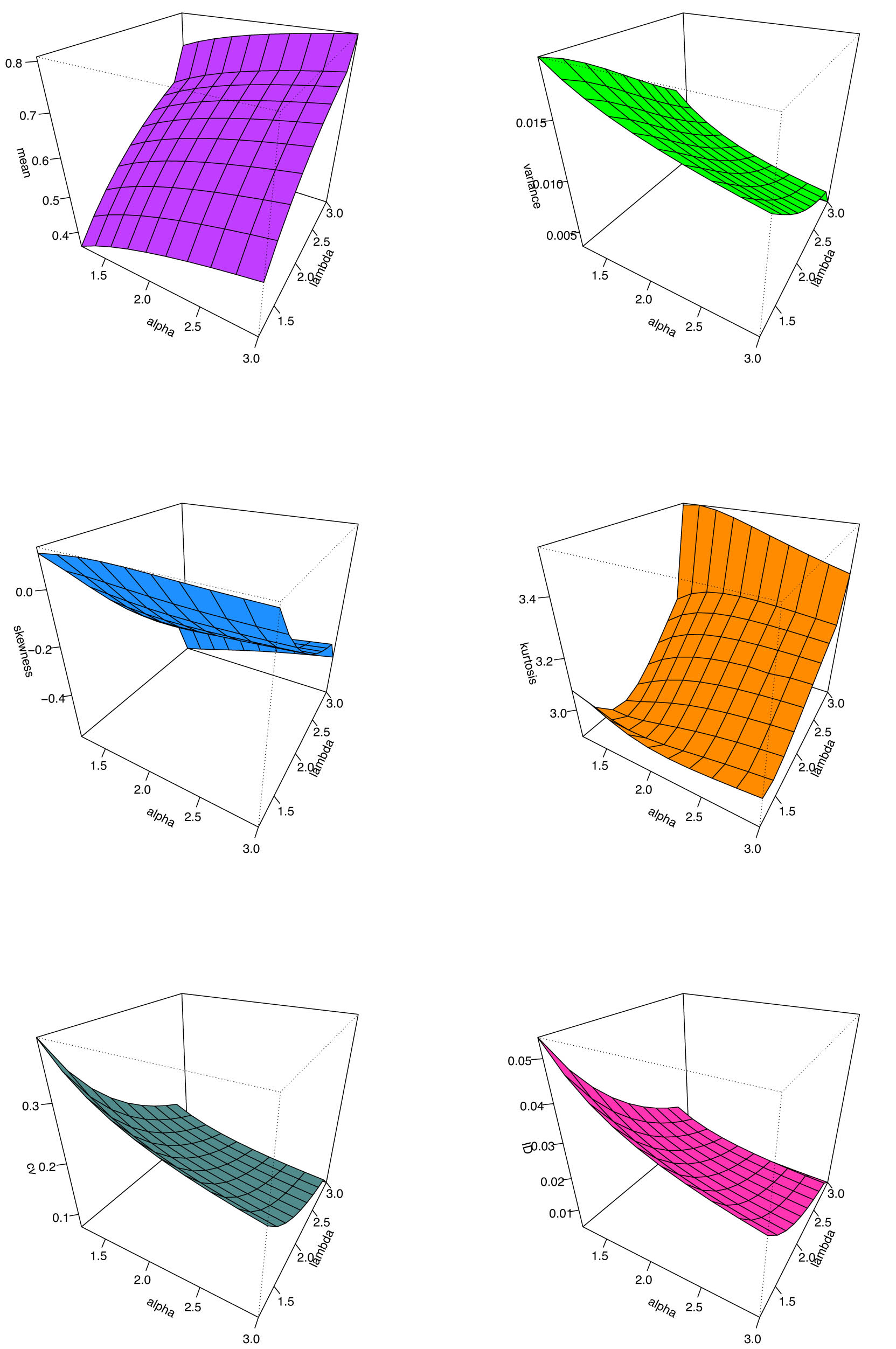
3D plots of the moments measurements for the SPB-X distribution at
3.3 Incomplete moments
The
where
3.4 Conditional moments
For the SPB-X model, the conditional moments defined by
where
and
4 Reliability measures
In this section, we suggested various significant reliability metrics for the SPB-X model, including common reliability functions, mean residual life function, mean waiting time function, residual moment, and reversed residual life.
4.1 Common reliability functions
The common reliability functions of SPB-X distribution are survival, hazard rate function (hrf), and reversed hrf, where the survival or reliability function is given by
The hrf is provided via
and reversed hrf is provided via
Figure 3 illustrates some hrf curves for the SPB-X distribution at
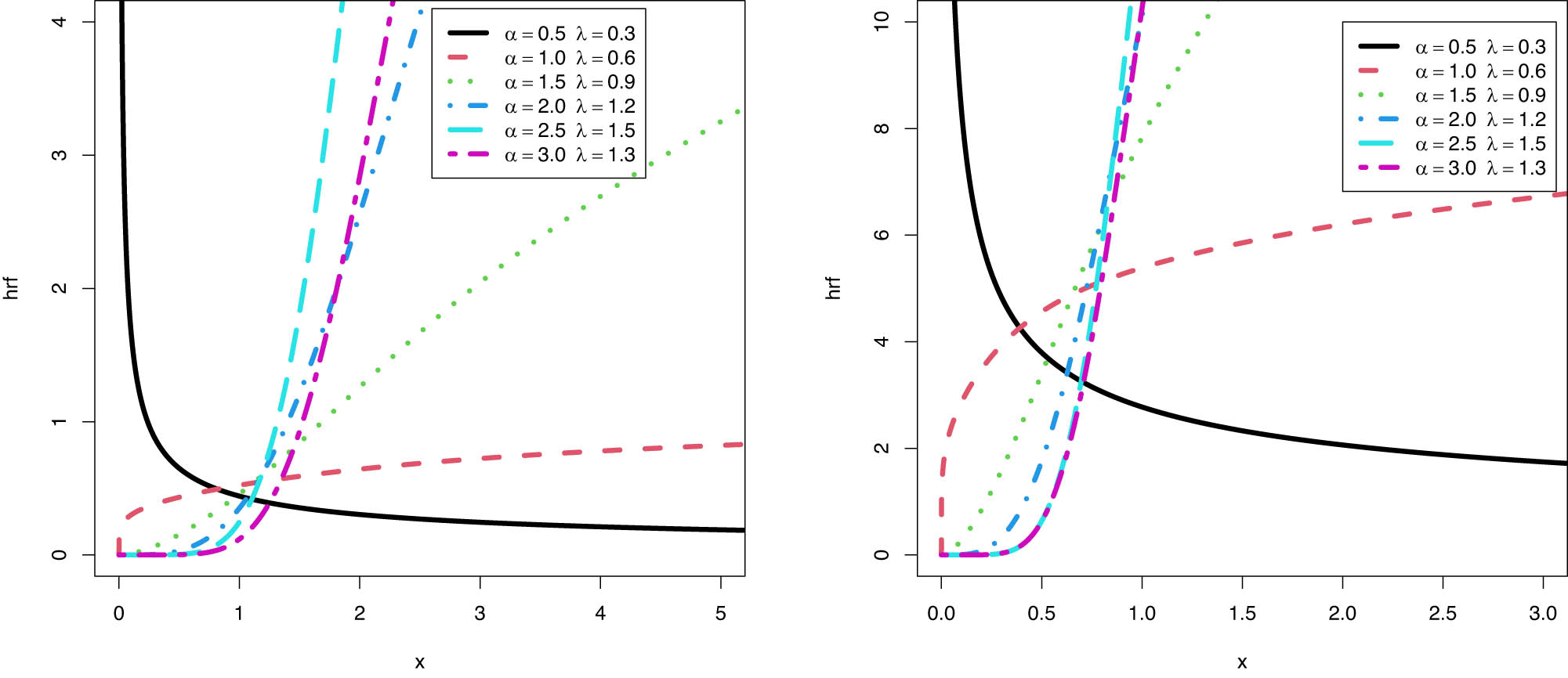
Plots of the hrf for the SPB-X distribution at
4.2 Mean residual life function
To characterize lifespan distributions, the mean residual life (MRL) function is of critical significance in the fields of dependability, survival analysis, actuarial sciences, economics, and social sciences. In addition, it is an essential component in the repair and replacement methods and provides a comprehensive summary of the residual life function. The MRL function may be derived for the SPB-X distribution from the following:
4.3 Mean inactivity time function
Given that
4.4 Moment of residual and reversed residual lifes
The residual life is the duration beyond
Employing (8) and utilizing the binomial expansion of
On the other hand, the
By utilizing (8) and employing the binomial expansion of
5 Actuarial measures
In actuarial practice, evaluating risk exposures is essential for companies. One of the primary goals of actuarial science institutes is to forecast market risks within a portfolio of instruments. Consequently, assessing risk measures is crucial in purchasing and selling products. In this section, we will explore many essential risk measures for the SPB-X distribution. These risk measures include the value at risk (VaR), the ES, the TVaR, the TV, and the TVP [47].
5.1 VaR measure
Risk managers often focus on the likelihood of an unfavorable result, which can be quantified using VaR at a certain probability level. The VaR [36] is used to assess risk exposure, thereby determining the capital required to endure undesirable outcomes. The VaR of the SPB-X distribution is specified as follows:
5.2 ES measure
Another significant financial metric is the ES, first articulated by [37,38]. The ES is a metric that provides superior justification for trading relative to VaR.
for
5.3 TVaR measure
The TVaR is a crucial risk metric. When an event occurs over a set probability threshold, TVaR is used to assess the expected value of the incurred loss. The TVaR of the SPB-X distribution is explicitly specified as follows:
5.4 TV measure
The TV risk measure, as put up by Landsman [39], is summarized as the variance of the loss distribution above a certain critical threshold. The TV of the SPB-X distribution may be characterized as follows:
where
5.5 TVP measure
The TVP is another important measure that plays an essential role in insurance sciences and is the mixture of central tendency and dispersion statistics. The TVP of SPB-X distribution takes the following form:
where
Key actuarial metrics, such as VaR, ES, Tail TVaR, TV, and TVP, are summarized in Table 3 for various combinations of
Actuarial measures for
|
|
|
|
VaR | ES | TVaR | TV | TVP | ||
|---|---|---|---|---|---|---|---|---|---|
|
|
|
|
|||||||
| 0.5 | 0.5 | 0.650 | 0.1008 | 0.0298 | 0.2774 | 0.0375 | 0.2961 | 0.3055 | 0.3112 |
| 0.700 | 0.1241 | 0.0357 | 0.3049 | 0.0385 | 0.3242 | 0.3338 | 0.3395 | ||
| 0.750 | 0.1531 | 0.0425 | 0.3383 | 0.0395 | 0.3580 | 0.3679 | 0.3738 | ||
| 0.800 | 0.1904 | 0.0505 | 0.3801 | 0.0405 | 0.4004 | 0.4105 | 0.4166 | ||
| 0.850 | 0.2408 | 0.0601 | 0.4354 | 0.0417 | 0.4563 | 0.4668 | 0.4730 | ||
| 0.900 | 0.3154 | 0.0721 | 0.5155 | 0.0432 | 0.5371 | 0.5479 | 0.5544 | ||
| 0.950 | 0.4498 | 0.0880 | 0.6567 | 0.0450 | 0.6792 | 0.6904 | 0.6972 | ||
| 0.975 | 0.5903 | 0.0989 | 0.8018 | 0.0463 | 0.8250 | 0.8365 | 0.8435 | ||
| 0.990 | 0.7821 | 0.1075 | 0.9976 | 0.0474 | 1.0213 | 1.0332 | 1.0403 | ||
| 0.995 | 0.9302 | 0.1113 | 1.1476 | 0.0481 | 1.1717 | 1.1837 | 1.1909 | ||
| 1.2 | 0.650 | 0.3211 | 0.1485 | 0.5605 | 0.0536 | 0.5873 | 0.6008 | 0.6088 | |
| 0.700 | 0.3601 | 0.1622 | 0.5972 | 0.0531 | 0.6238 | 0.6371 | 0.6450 | ||
| 0.750 | 0.4054 | 0.1768 | 0.6403 | 0.0526 | 0.6666 | 0.6797 | 0.6876 | ||
| 0.800 | 0.4597 | 0.1928 | 0.6924 | 0.0521 | 0.7185 | 0.7315 | 0.7393 | ||
| 0.850 | 0.5285 | 0.2104 | 0.7590 | 0.0516 | 0.7848 | 0.7977 | 0.8055 | ||
| 0.900 | 0.6237 | 0.2305 | 0.8521 | 0.0510 | 0.8776 | 0.8903 | 0.8980 | ||
| 0.950 | 0.7835 | 0.2550 | 1.0094 | 0.0504 | 1.0346 | 1.0472 | 1.0548 | ||
| 0.975 | 0.9409 | 0.2703 | 1.1656 | 0.0499 | 1.1906 | 1.2031 | 1.2106 | ||
| 0.990 | 1.1473 | 0.2818 | 1.3708 | 0.0498 | 1.3957 | 1.4082 | 1.4156 | ||
| 0.995 | 1.3025 | 0.2865 | 1.5257 | 0.0496 | 1.5505 | 1.5629 | 1.5703 | ||
| 1.6 | 0.5 | 0.650 | 0.4882 | 0.2854 | 0.6440 | 0.0146 | 0.6513 | 0.6549 | 0.6571 |
| 0.700 | 0.5210 | 0.3010 | 0.6672 | 0.0133 | 0.6738 | 0.6772 | 0.6792 | ||
| 0.750 | 0.5564 | 0.3169 | 0.6929 | 0.0120 | 0.6989 | 0.7019 | 0.7037 | ||
| 0.800 | 0.5956 | 0.3330 | 0.7223 | 0.0107 | 0.7276 | 0.7303 | 0.7319 | ||
| 0.850 | 0.6409 | 0.3498 | 0.7571 | 0.0093 | 0.7618 | 0.7641 | 0.7655 | ||
| 0.900 | 0.6973 | 0.3674 | 0.8018 | 0.0078 | 0.8057 | 0.8077 | 0.8089 | ||
| 0.950 | 0.7791 | 0.3868 | 0.8689 | 0.0060 | 0.8719 | 0.8735 | 0.8744 | ||
| 0.975 | 0.8482 | 0.3976 | 0.9272 | 0.0050 | 0.9297 | 0.9309 | 0.9317 | ||
| 0.990 | 0.9261 | 0.4050 | 0.9946 | 0.0042 | 0.9967 | 0.9977 | 0.9983 | ||
| 0.995 | 0.9776 | 0.4077 | 1.0409 | 0.0028 | 1.0423 | 1.0430 | 1.0434 | ||
| 1.2 | 0.650 | 0.7012 | 0.5220 | 0.8222 | 0.0089 | 0.8266 | 0.8289 | 0.8302 | |
| 0.700 | 0.7268 | 0.5357 | 0.8402 | 0.0082 | 0.8443 | 0.8463 | 0.8475 | ||
| 0.750 | 0.7541 | 0.5493 | 0.8601 | 0.0074 | 0.8638 | 0.8657 | 0.8668 | ||
| 0.800 | 0.7844 | 0.5631 | 0.8830 | 0.0066 | 0.8863 | 0.8879 | 0.8889 | ||
| 0.850 | 0.8193 | 0.5771 | 0.9102 | 0.0058 | 0.9131 | 0.9145 | 0.9154 | ||
| 0.900 | 0.8629 | 0.5917 | 0.9451 | 0.0051 | 0.9476 | 0.9489 | 0.9497 | ||
| 0.950 | 0.9266 | 0.6075 | 0.9985 | 0.0039 | 1.0004 | 1.0014 | 1.0020 | ||
| 0.975 | 0.9812 | 0.6163 | 1.0455 | 0.0032 | 1.0471 | 1.0480 | 1.0484 | ||
| 0.990 | 1.0439 | 0.6222 | 1.1008 | 0.0027 | 1.1022 | 1.1028 | 1.1033 | ||
| 0.995 | 1.0861 | 0.6245 | 1.1384 | 0.0028 | 1.1398 | 1.1405 | 1.1409 | ||
6 Estimation methods
6.1 Maximum likelihood estimation (MLE)
The MLEs [45,58] is the most widely used method of parameter estimation. Let
To obtain the MLEs of parameters, we differentiate (19) partially with respect to
and
Then the maximum likelihood estimates of the parameters
6.2 Least squares estimators (LSEs)
The LSEs [46,48,49] are key in regression and estimation analysis, with the aim of minimizing the squared differences between observed and predicted values. In linear regression, LSE finds the coefficients that best fit the data. For a RS
This minimization aims to identify the optimal values of
6.3 MPS
MPS estimators are vital in statistical inference, offering efficient parameter estimates for probability distributions, especially useful in survival analysis and reliability modeling with censored data. In survival analysis, where not all failure times in a sample are fully observed, MPS estimators effectively manage such censoring. The method involves MPS between observed failure times to estimate distribution parameters. These estimators are recognized for their robustness against outliers and their strong performance across various distributional assumptions. MPS estimators are widely used in different fields. Further discussions on MPS can be found in papers by previous studies [43,44, 50,51].
The MPS estimators for
where
6.4 Bayesian estimation
In this subsection, we utilize the Bayesian estimation method to estimate the unknown parameters of the SPB-X distribution. The core concept of the Bayesian approach is that the model’s parameters are treated as random variables with a predefined distribution, known as the prior distribution. When prior knowledge is available, selecting an appropriate prior is essential. We choose the gamma conjugate prior for the parameters due to several reasons, such as its flexibility, noninformative nature, and the simplicity, it offers in analytical or computational updates to the posterior. In addition, its positive domain makes it well suited for modeling parameters. We implement the Bayesian inference method to estimate the unknown parameters
The estimates have been derived using the square error loss function. Therefore, the joint prior density of the independent parameters is expressed as follows:
and
where
Since Eq. (24) cannot be solved explicitly, numerical methods are used. One of the most effective numerical approaches in Bayesian estimation is the Monte Carlo Markov chain method. In this case, we propose using the Metropolis–Hastings algorithm, see the study by Tierney [59].
7 Simulation
The simulation of four estimation methods deepens our understanding of statistical techniques, assists in choosing the most appropriate method, and reveals the strengths and weaknesses of various approaches in different contexts. This section utilizes simulation analysis to compare the results of three different parameter estimates for the SPB-X distribution. We carried out simulations by generating 10,000 RS with sizes of
Simulations allow researchers to assess the performance of various estimation methods under different conditions. By generating synthetic datasets with known properties, they can evaluate the accuracy, rank, RMSE, and RAB of each technique.
Simulations serve as a tool to optimize estimation techniques for the parameters of the SPB-X distribution. Researchers can adjust the algorithm parameters or experiment with alternative methodologies to determine the most efficient and accurate approach for specific scenarios.
Through simulation studies, researchers can systematically compare multiple estimators for the SPB-X distribution parameters within a controlled setting. This facilitates an objective assessment of each method’s advantages and limitations, guiding the selection of the most suitable estimator for practical use.
RAB, RMSE, and ranked of estimation methods for parameters of SPB-X distribution
|
|
MLE | LS | MPS | Bayeaisan | ||||||||||||||
|---|---|---|---|---|---|---|---|---|---|---|---|---|---|---|---|---|---|---|
|
|
n | RAB | RMSE | RAB | RMSE | RAB | RMSE | RAB | RMSE | |||||||||
| 1.5 | 25 |
|
0.098349 | 1 | 0.535404 | 1 | 0.008759 | 4 | 0.16359 | 4 | 0.028028 | 3 | 0.525338 | 2 | 0.096516 | 2 | 0.497735 | 3 |
|
|
0.087211 | 1 | 0.159227 | 1 |
|
4 | 0.083594 | 4 | 0.086144 | 2 | 0.14988 | 2 | 0.03257 | 3 | 0.12008 | 3 | ||
|
|
0.014938 | 3 | 0.212967 | 1 | 0.006078 | 4 | 0.130798 | 4 | 0.018591 | 2 | 0.186292 | 2 | 0.063172 | 1 | 0.142277 | 3 | ||
|
|
5 | 3 | 12 | 12 | 7 | 6 | 6 | 9 | ||||||||||
| 70 |
|
0.064606 | 2 | 0.517576 | 1 | 0.004599 | 4 | 0.099651 | 4 | 0.01644 | 3 | 0.325084 | 3 | 0.085276 | 1 | 0.398442 | 2 | |
|
|
0.082028 | 1 | 0.140715 | 1 | 0.006724 | 4 | 0.042627 | 4 | 0.010017 | 3 | 0.090501 | 3 | 0.026713 | 2 | 0.099203 | 2 | ||
|
|
|
3 | 0.084148 | 1 |
|
4 | 0.075748 | 2 |
|
4 | 0.081042 | 3 | 0.024655 | 1 | 0.081247 | 2 | ||
|
|
6 | 3 | 12 | 10 | 10 | 9 | 4 | 6 | ||||||||||
| 100 |
|
0.016829 | 2 | 0.453821 | 1 |
|
4 | 0.085145 | 4 | 0.015741 | 3 | 0.301315 | 3 | 0.059674 | 1 | 0.389176 | 2 | |
|
|
0.016211 | 1 | 0.124052 | 1 | 0.003828 | 4 | 0.036019 | 4 | 0.009168 | 3 | 0.084335 | 3 | 0.015022 | 2 | 0.091723 | 2 | ||
|
|
|
3 | 0.080529 | 1 |
|
4 | 0.065027 | 2 |
|
4 | 0.079522 | 2 | 0.008973 | 1 | 0.071036 | 3 | ||
|
|
6 | 3 | 12 | 10 | 10 | 8 | 4 | 7 | ||||||||||
| 200 |
|
0.014146 | 2 | 0.241456 | 1 |
|
4 | 0.031091 | 4 | 0.014128 | 3 | 0.166741 | 2 | 0.030725 | 1 | 0.128756 | 3 | |
|
|
0.002011 | 3 | 0.066863 | 1 | 0.000717 | 4 | 0.02494 | 4 | 0.0082 | 1 | 0.051008 | 3 | 0.005046 | 2 | 0.052854 | 2 | ||
|
|
|
3 | 0.076778 | 1 |
|
4 | 0.047154 | 2 |
|
4 | 0.06048 | 3 | 0.008912 | 1 | 0.068712 | 2 | ||
|
|
8 | 3 | 12 | 10 | 8 | 8 | 4 | 7 | ||||||||||
| Total rank | 11 | 22 | 16 | 11 | ||||||||||||||
| 0.5 | 25 |
|
0.337683 | 1 | 0.50644 | 1 | 0.090933 | 4 | 0.146 | 4 | 0.336589 | 2 | 0.45835 | 2 | 0.217261 | 3 | 0.258538 | 3 |
|
|
0.111395 | 1 | 0.297497 | 1 | 0.036013 | 4 | 0.166826 | 4 | 0.110824 | 2 | 0.265625 | 2 | 0.100963 | 3 | 0.179842 | 3 | ||
|
|
|
4 | 0.395424 | 1 |
|
4 | 0.143998 | 2 |
|
3 | 0.313146 | 2 |
|
1 | 0.20029 | 3 | ||
|
|
6 | 3 | 12 | 10 | 7 | 6 | 7 | 9 | ||||||||||
| 70 |
|
0.207274 | 1 | 0.26776 | 2 | 0.05815 | 4 | 0.109132 | 4 | 0.206881 | 2 | 0.301125 | 1 | 0.124303 | 3 | 0.1626 | 3 | |
|
|
0.090973 | 1 | 0.194696 | 1 | 0.034912 | 4 | 0.095431 | 4 | 0.090931 | 2 | 0.192916 | 2 | 0.076127 | 3 | 0.118987 | 3 | ||
|
|
|
3 | 0.284272 | 1 |
|
4 | 0.120023 | 2 |
|
4 | 0.220632 | 2 | 0.001959 | 1 | 0.150957 | 3 | ||
|
|
5 | 4 | 12 | 10 | 8 | 5 | 7 | 9 | ||||||||||
| 100 |
|
0.192792 | 2 | 0.247364 | 2 |
|
4 | 0.066954 | 4 | 0.193514 | 1 | 0.261325 | 1 | 0.100436 | 3 | 0.156027 | 3 | |
|
|
0.089484 | 2 | 0.176863 | 1 |
|
4 | 0.090415 | 4 | 0.089562 | 1 | 0.176665 | 2 | 0.046063 | 3 | 0.109306 | 3 | ||
|
|
|
4 | 0.229272 | 1 | 0.018205 | 4 | 0.072571 | 1 |
|
3 | 0.202952 | 2 | 0.001209 | 2 | 0.134832 | 3 | ||
|
|
8 | 4 | 12 | 9 | 5 | 5 | 8 | 9 | ||||||||||
| 200 |
|
0.149399 | 1 | 0.185062 | 2 |
|
4 | 0.024367 | 4 | 0.148784 | 2 | 0.188903 | 1 | 0.043033 | 3 | 0.092727 | 3 | |
|
|
0.080922 | 1 | 0.148105 | 1 |
|
4 | 0.030511 | 4 | 0.07918 | 2 | 0.13829 | 2 | 0.018522 | 3 | 0.077706 | 3 | ||
|
|
|
4 | 0.202376 | 1 |
|
4 | 0.030395 | 2 |
|
3 | 0.157082 | 2 | 0.001143 | 1 | 0.10759 | 3 | ||
|
|
6 | 4 | 12 | 10 | 7 | 5 | 7 | 9 | ||||||||||
| Total rank | 10 | 22 | 12 | 16 | ||||||||||||||
|
|
21 | 44 | 28 | 27 | ||||||||||||||
RAB, RMSE, and ranked of estimation methods for parameters of SPB-X distribution
|
|
MLE | LS | MPS | Bayeaisan | ||||||||||||||
|---|---|---|---|---|---|---|---|---|---|---|---|---|---|---|---|---|---|---|
|
|
|
RAB | RMSE | RAB | RMSE | RAB | RMSE | RAB | RMSE | |||||||||
| 0.5 | 25 |
|
0.237293 | 1 | 0.481939 | 1 | 0.031422 | 4 | 0.140239 | 4 | 0.236122 | 2 | 0.369424 | 2 | 0.148007 | 3 | 0.178753 | 3 |
|
|
0.094034 | 1 | 0.313662 | 1 |
|
3 | 0.159829 | 4 | 0.079784 | 2 | 0.249774 | 2 | 0.069063 | 3 | 0.122545 | 4 | ||
|
|
|
3 | 0.56169 | 1 |
|
4 | 0.191695 | 4 |
|
2 | 0.487931 | 2 |
|
1 | 0.246092 | 3 | ||
|
|
5 | 3 | 11 | 12 | 6 | 6 | 7 | 10 | ||||||||||
| 70 |
|
0.135257 | 2 | 0.290683 | 1 | 0.030646 | 4 | 0.086505 | 4 | 0.135534 | 1 | 0.230553 | 2 | 0.071858 | 3 | 0.10814 | 3 | |
|
|
0.065682 | 2 | 0.188634 | 1 | 0.010859 | 3 | 0.083362 | 4 | 0.065696 | 1 | 0.154763 | 2 | 0.035749 | 3 | 0.081059 | 4 | ||
|
|
|
4 | 0.463898 | 1 |
|
4 | 0.166698 | 2 |
|
3 | 0.392399 | 2 |
|
1 | 0.215204 | 3 | ||
|
|
8 | 3 | 11 | 10 | 5 | 6 | 7 | 10 | ||||||||||
| 100 |
|
0.108458 | 1 | 0.191718 | 1 |
|
4 | 0.068469 | 4 | 0.108304 | 2 | 0.181584 | 2 | 0.059705 | 3 | 0.097331 | 3 | |
|
|
0.059619 | 1 | 0.129028 | 1 |
|
4 | 0.068863 | 4 | 0.059537 | 2 | 0.126247 | 2 | 0.033491 | 3 | 0.078193 | 3 | ||
|
|
|
4 | 0.373276 | 1 | 0.004215 | 4 | 0.0915 | 1 |
|
3 | 0.345385 | 2 |
|
2 | 0.204391 | 3 | ||
|
|
6 | 3 | 12 | 9 | 7 | 6 | 8 | 9 | ||||||||||
| 200 |
|
0.080716 | 1 | 0.065794 | 2 | 0.002218 | 4 | 0.038939 | 4 | 0.080353 | 2 | 0.12508 | 1 | 0.043635 | 3 | 0.060712 | 3 | |
|
|
0.053007 | 1 | 0.058535 | 2 |
|
4 | 0.038808 | 4 | 0.052625 | 2 | 0.096398 | 1 | 0.028389 | 3 | 0.050202 | 3 | ||
|
|
|
4 | 0.184168 | 2 | 0.00109 | 4 | 0.040365 | 1 |
|
3 | 0.292117 | 1 |
|
2 | 0.179928 | 3 | ||
|
|
6 | 6 | 12 | 9 | 7 | 3 | 8 | 9 | ||||||||||
| Total rank | 12 | 21 | 10 | 17 | ||||||||||||||
| 1.5 | 25 |
|
|
4 | 0.533336 | 1 |
|
4 | 0.214276 | 2 |
|
3 | 0.434168 | 2 | 0.041754 | 1 | 0.420127 | 3 |
|
|
|
3 | 0.225968 | 1 |
|
3 | 0.200131 | 4 |
|
2 | 0.203626 | 2 | 0.005053 | 1 | 0.082185 | 4 | ||
|
|
|
4 | 0.416789 | 1 | 0.058698 | 3 | 0.228875 | 1 |
|
3 | 0.355903 | 2 | 0.002684 | 2 | 0.208831 | 4 | ||
|
|
11 | 3 | 10 | 7 | 8 | 6 | 4 | 11 | ||||||||||
| 70 |
|
0.036452 | 1 | 0.153281 | 2 |
|
4 | 0.115467 | 4 | 0.00494 | 3 | 0.385402 | 1 | 0.034544 | 2 | 0.131382 | 3 | |
|
|
|
4 | 0.151305 | 2 |
|
3 | 0.12475 | 2 |
|
3 | 0.163303 | 1 | 0.004341 | 1 | 0.065997 | 4 | ||
|
|
|
2 | 0.143572 | 2 |
|
4 | 0.123425 | 4 |
|
3 | 0.292842 | 1 | 0.002335 | 1 | 0.129063 | 3 | ||
|
|
7 | 6 | 11 | 10 | 9 | 3 | 4 | 10 | ||||||||||
| 100 |
|
0.019642 | 2 | 0.125253 | 2 |
|
4 | 0.08095 | 4 | 0.00382 | 3 | 0.344566 | 1 | 0.031589 | 1 | 0.123064 | 3 | |
|
|
|
3 | 0.137042 | 1 |
|
3 | 0.093568 | 4 |
|
2 | 0.136492 | 2 | 0.003622 | 1 | 0.060676 | 4 | ||
|
|
|
3 | 0.12584 | 2 | 0.001803 | 3 | 0.109926 | 1 |
|
4 | 0.271943 | 1 |
|
2 | 0.108031 | 4 | ||
|
|
8 | 5 | 10 | 9 | 9 | 4 | 4 | 11 | ||||||||||
| 200 |
|
0.017144 | 2 | 0.123611 | 2 |
|
4 | 0.070877 | 4 | 0.00276 | 3 | 0.300586 | 1 | 0.023573 | 1 | 0.092434 | 3 | |
|
|
0.008163 | 2 | 0.105762 | 1 |
|
3 | 0.081686 | 4 | 0.008167 | 1 | 0.089414 | 2 | 0.001453 | 3 | 0.055692 | 4 | ||
|
|
|
3 | 0.112907 | 2 |
|
4 | 0.086068 | 2 |
|
4 | 0.222332 | 1 |
|
1 | 0.091578 | 3 | ||
|
|
7 | 5 | 11 | 10 | 8 | 4 | 5 | 10 | ||||||||||
| Total rank | 12 | 21 | 12 | 15 | ||||||||||||||
|
|
24 | 42 | 22 | 32 | ||||||||||||||
RAB, RMSE, and ranked of estimation methods for parameters of SPB-X distribution
|
|
MLE | LS | MPS | Bayeaisan | ||||||||||||||
|---|---|---|---|---|---|---|---|---|---|---|---|---|---|---|---|---|---|---|
|
|
|
RAB | RMSE | RAB | RMSE | RAB | RMSE | RAB | RMSE | |||||||||
| 2 | 25 |
|
|
4 | 0.784902 | 1 |
|
4 | 0.186499 | 3 |
|
2 | 0.618933 | 2 | 0.0798 | 1 | 0.452759 | 3 |
|
|
|
4 | 0.36032 | 1 |
|
2 | 0.286095 | 2 |
|
3 | 0.274264 | 3 | 0.0082 | 1 | 0.191702 | 4 | ||
|
|
0.038 | 2 | 0.756547 | 1 |
|
4 | 0.203331 | 4 | 0.0385 | 1 | 0.599379 | 2 |
|
3 | 0.249373 | 3 | ||
|
|
10 | 3 | 10 | 9 | 6 | 7 | 5 | 10 | ||||||||||
| 70 |
|
|
4 | 0.675556 | 1 | 0.006 | 4 | 0.178961 | 2 |
|
3 | 0.402374 | 2 | 0.052 | 1 | 0.323463 | 3 | |
|
|
|
3 | 0.203099 | 1 |
|
2 | 0.19451 | 2 |
|
4 | 0.163596 | 3 | 0.0068 | 1 | 0.110154 | 4 | ||
|
|
0.0093 | 1 | 0.711175 | 1 |
|
4 | 0.169255 | 4 | 0.0088 | 2 | 0.353533 | 2 | 0.0037 | 3 | 0.213583 | 3 | ||
|
|
8 | 3 | 10 | 8 | 9 | 7 | 5 | 10 | ||||||||||
| 100 |
|
0.0069 | 2 | 0.466559 | 1 |
|
4 | 0.13176 | 4 | 0.0069 | 2 | 0.361317 | 2 | 0.044 | 1 | 0.295145 | 3 | |
|
|
|
4 | 0.172465 | 1 | 0.0039 | 2 | 0.168627 | 2 |
|
3 | 0.135038 | 3 | 0.0055 | 1 | 0.084145 | 4 | ||
|
|
0.0084 | 1 | 0.553203 | 1 | 0.002 | 4 | 0.142907 | 4 | 0.0075 | 2 | 0.314431 | 2 | 0.0035 | 3 | 0.204128 | 3 | ||
|
|
7 | 3 | 10 | 10 | 7 | 7 | 5 | 10 | ||||||||||
| 200 |
|
|
3 | 0.452244 | 1 | 0.0043 | 4 | 0.128513 | 2 |
|
3 | 0.26335 | 3 | 0.0434 | 1 | 0.26658 | 2 | |
|
|
|
3 | 0.109653 | 1 |
|
2 | 0.107198 | 2 |
|
4 | 0.093364 | 3 | 0.0055 | 1 | 0.058806 | 4 | ||
|
|
0.0025 | 1 | 0.499037 | 1 |
|
4 | 0.134906 | 4 | 0.0021 | 3 | 0.237421 | 2 | 0.0025 | 1 | 0.191229 | 3 | ||
|
|
7 | 3 | 10 | 8 | 10 | 8 | 3 | 9 | ||||||||||
| Total rank | 10 | 18 | 18 | 12 | ||||||||||||||
| 4 | 25 |
|
0.0987 | 1 | 0.807114 | 1 |
|
3 | 0.480387 | 4 | 0.0206 | 3 | 0.603981 | 2 | 0.056 | 2 | 0.442574 | 4 |
|
|
|
3 | 0.90611 | 1 |
|
4 | 0.443569 | 1 |
|
4 | 0.68943 | 2 |
|
2 | 0.46061 | 3 | ||
|
|
0.0096 | 2 | 0.416854 | 1 | 0.0241 | 4 | 0.1636 | 1 | 0.0057 | 3 | 0.402546 | 2 | 0.0028 | 4 | 0.210831 | 3 | ||
|
|
6 | 3 | 11 | 6 | 10 | 6 | 8 | 10 | ||||||||||
| 70 |
|
0.015 | 2 | 0.405756 | 2 |
|
4 | 0.253711 | 4 | 0.0145 | 3 | 0.429374 | 1 | 0.0523 | 1 | 0.359802 | 3 | |
|
|
|
4 | 0.725479 | 1 |
|
4 | 0.243816 | 2 |
|
3 | 0.462748 | 2 |
|
1 | 0.380727 | 3 | ||
|
|
|
4 | 0.396709 | 1 | 0.0134 | 4 | 0.123397 | 1 |
|
3 | 0.284519 | 2 |
|
2 | 0.185777 | 3 | ||
|
|
10 | 4 | 12 | 7 | 9 | 5 | 4 | 9 | ||||||||||
| 100 |
|
0.014 | 2 | 0.327157 | 2 |
|
4 | 0.212561 | 4 | 0.0136 | 3 | 0.382202 | 1 | 0.0466 | 1 | 0.314589 | 3 | |
|
|
|
4 | 0.306385 | 2 |
|
4 | 0.18737 | 2 |
|
3 | 0.385213 | 1 | 0.0014 | 1 | 0.306162 | 3 | ||
|
|
|
4 | 0.155957 | 2 | 0.0061 | 4 | 0.058291 | 1 |
|
3 | 0.227913 | 1 |
|
2 | 0.149529 | 3 | ||
|
|
10 | 6 | 12 | 7 | 9 | 3 | 4 | 9 | ||||||||||
| 200 |
|
0.0141 | 2 | 0.323692 | 1 |
|
4 | 0.187806 | 4 | 0.0124 | 3 | 0.28776 | 2 | 0.0426 | 1 | 0.266214 | 3 | |
|
|
|
4 | 0.290651 | 2 |
|
4 | 0.175217 | 1 |
|
3 | 0.302992 | 1 |
|
2 | 0.229806 | 3 | ||
|
|
|
3 | 0.13804 | 2 | 0.0051 | 4 | 0.046913 | 1 |
|
4 | 0.189102 | 1 |
|
2 | 0.126885 | 3 | ||
|
|
9 | 5 | 12 | 6 | 10 | 4 | 5 | 9 | ||||||||||
| Total rank | 14 | 18 | 14 | 14 | ||||||||||||||
|
|
24 | 36 | 32 | 26 | ||||||||||||||
RAB, RMSE, and ranked of estimation methods for parameters of SPB-X distribution
|
|
MLE | LS | MPS | Bayeaisan | ||||||||||||||
|---|---|---|---|---|---|---|---|---|---|---|---|---|---|---|---|---|---|---|
|
|
|
RAB | RMSE | RAB | RMSE | RAB | RMSE | RAB | RMSE | |||||||||
| 1.5 | 25 |
|
|
4 |
|
1 |
|
3 |
|
2 | 1.022988 | 1 | 0.247263 | 4 | 0.749682 | 2 | 0.65512 | 3 |
|
|
|
3 |
|
2 |
|
4 |
|
1 | 0.171082 | 2 | 0.263046 | 1 | 0.142879 | 3 | 0.124047 | 4 | ||
|
|
0.03102 | 1 |
|
4 | 0.030965 | 2 | 0.011691 | 3 | 0.721195 | 1 | 0.274253 | 3 | 0.431103 | 2 | 0.210736 | 4 | ||
|
|
8 | 7 | 9 | 6 | 4 | 8 | 7 | 11 | ||||||||||
| 70 |
|
|
4 |
|
2 |
|
3 | 0.021909 | 1 | 0.203063 | 3 | 0.164013 | 4 | 0.601484 | 2 | 0.617428 | 1 | |
|
|
|
4 |
|
1 |
|
3 |
|
2 | 0.063614 | 4 | 0.070686 | 3 | 0.099399 | 1 | 0.085748 | 2 | ||
|
|
0.021379 | 1 |
|
4 | 0.0211 | 2 | 0.005284 | 3 | 0.148033 | 4 | 0.165576 | 3 | 0.292466 | 1 | 0.175084 | 2 | ||
|
|
9 | 7 | 8 | 6 | 11 | 10 | 4 | 5 | ||||||||||
| 100 |
|
|
4 |
|
2 |
|
3 | 0.005074 | 1 | 0.20064 | 3 | 0.153381 | 4 | 0.500061 | 2 | 0.567637 | 1 | |
|
|
|
3 |
|
1 |
|
4 |
|
2 | 0.061136 | 3 | 0.06013 | 4 | 0.078926 | 1 | 0.078552 | 2 | ||
|
|
0.018067 | 1 | 0.001437 | 4 | 0.01782 | 2 | 0.004198 | 3 | 0.127727 | 4 | 0.139024 | 3 | 0.226073 | 1 | 0.167588 | 2 | ||
|
|
8 | 7 | 9 | 6 | 10 | 11 | 4 | 5 | ||||||||||
| 200 |
|
|
4 |
|
1 |
|
3 |
|
2 | 0.186027 | 3 | 0.148856 | 4 | 0.36416 | 2 | 0.522604 | 1 | |
|
|
|
4 |
|
1 |
|
3 |
|
2 | 0.060114 | 2 | 0.043521 | 4 | 0.055014 | 3 | 0.062995 | 1 | ||
|
|
0.005953 | 1 |
|
4 | 0.005789 | 2 | 0.004023 | 3 | 0.052092 | 4 | 0.100627 | 3 | 0.147558 | 2 | 0.153146 | 1 | ||
|
|
9 | 6 | 8 | 7 | 9 | 11 | 7 | 3 | ||||||||||
| 1.5 | Total rank | 15 | 15 | 20 | 10 | |||||||||||||
| 3 | 25 |
|
|
3 |
|
1 |
|
4 |
|
2 | 1.01585 | 1 | 0.304876 | 4 | 0.685717 | 2 | 0.670245 | 3 |
|
|
|
3 |
|
2 |
|
4 |
|
1 | 0.281515 | 2 | 0.322409 | 1 | 0.134832 | 3 | 0.123108 | 4 | ||
|
|
|
3 |
|
4 |
|
2 | 0.00603 | 1 | 0.954966 | 1 | 0.464819 | 3 | 0.569249 | 2 | 0.250907 | 4 | ||
|
|
9 | 7 | 10 | 4 | 4 | 8 | 7 | 11 | ||||||||||
| 70 |
|
|
4 |
|
2 |
|
3 | 0.011103 | 1 | 0.206847 | 3 | 0.111765 | 4 | 0.553092 | 1 | 0.545158 | 2 | |
|
|
|
4 |
|
2 |
|
3 |
|
1 | 0.194985 | 1 | 0.152068 | 2 | 0.093001 | 3 | 0.088362 | 4 | ||
|
|
0.002145 | 2 |
|
4 | 0.001838 | 3 | 0.002758 | 1 | 0.247989 | 2 | 0.22598 | 3 | 0.397819 | 1 | 0.219657 | 4 | ||
|
|
10 | 8 | 9 | 3 | 6 | 9 | 5 | 10 | ||||||||||
| 100 |
|
|
3 |
|
2 |
|
4 | 0.010222 | 1 | 0.189243 | 3 | 0.102759 | 4 | 0.481484 | 2 | 0.511498 | 1 | |
|
|
|
4 |
|
2 |
|
3 | 0.001072 | 1 | 0.156499 | 1 | 0.148069 | 2 | 0.078632 | 3 | 0.075901 | 4 | ||
|
|
0.001646 | 3 |
|
4 | 0.001779 | 1 | 0.001779 | 2 | 0.142582 | 4 | 0.216851 | 3 | 0.344835 | 1 | 0.220094 | 2 | ||
|
|
10 | 8 | 8 | 4 | 8 | 9 | 6 | 7 | ||||||||||
| 200 |
|
|
3 |
|
2 |
|
4 | 0.009103 | 1 | 0.146666 | 3 | 0.091199 | 4 | 0.367609 | 2 | 0.413775 | 1 | |
|
|
|
3 |
|
2 |
|
4 |
|
1 | 0.152245 | 1 | 0.043352 | 4 | 0.054523 | 3 | 0.055331 | 2 | ||
|
|
0.000397 | 3 | 0.000944 | 2 | 0.000335 | 4 | 0.001427 | 1 | 0.137847 | 4 | 0.159341 | 3 | 0.251225 | 1 | 0.186038 | 2 | ||
|
|
9 | 6 | 12 | 3 | 8 | 11 | 6 | 5 | ||||||||||
| Total rank | 15 | 15 | 19 | 11 | ||||||||||||||
|
|
30 | 30 | 39 | 21 | ||||||||||||||
The best-performing estimation method can be determined using the total rank column in the table. The method with the highest total rank is considered the most effective in different scenarios. Based on the ranked values provided in the table, it is clear which method consistently achieves better performance in terms of RMSE and RAB. In the case of
In all cases, the LS method achieved the highest total rank, reaching 546, indicating its superior performance. The Bayesian method followed with a total rank of 494. However, the MLE method had the lowest performance, with a total rank of 327, making it the least effective among the estimation methods compared.
7.1 Approximate confidence intervals (ACIs)
Determining the exact distribution of these estimates becomes problematic when closed-form MLEs and MPS for the unknown parameters cannot be obtained. Therefore, it is not feasible to obtain precise confidence intervals (CIs) for the parameters. Hence, ACIs are built using large sample approximation approaches for the parameters
Using the asymptotic normality features of MLEs and MPS, one may compute the ACIs for
From there, we can obtain the approximate asymptotic variance–covariance matrix, which is:
With a mean of
The
Tables 8 and 9 present confidence intervals for the parameters (
Confidence intervals for parameters of SPB-X distribution
|
|
|
||||||||||||||
|---|---|---|---|---|---|---|---|---|---|---|---|---|---|---|---|
| MLE | MPS | MLE | MPS | ||||||||||||
|
|
|
Lower | Upper | LACI | Lower | Upper | LACI |
|
Lower | Upper | LACI | Lower | Upper | LACI | |
| 1.5 | 25 |
|
0.6388 | 2.6563 | 2.0175 | 0.5157 | 2.5684 | 2.0527 | 0.5 | 0.0699 | 1.1674 | 1.0975 | 0.0416 | 1.3042 | 1.3722 |
|
|
0.2435 | 0.8438 | 0.6003 | 0.2617 | 0.8244 | 0.5627 | 0.1030 | 0.9910 | 0.8880 | 0.0566 | 1.0232 | 0.9665 | |||
|
|
0.3444 | 1.1780 | 0.8337 | 0.3998 | 1.1281 | 0.7282 | 0.7828 | 2.8879 | 2.1051 | 0.9352 | 2.7361 | 1.8010 | |||
| 70 |
|
0.6004 | 2.5934 | 1.9930 | 0.8893 | 2.1600 | 1.2707 | 0.0135 | 1.1217 | 1.1082 | 0.1358 | 0.9997 | 0.8638 | ||
|
|
0.2772 | 0.8048 | 0.5277 | 0.3279 | 0.6821 | 0.3542 | 0.1688 | 0.8969 | 0.7282 | 0.2364 | 0.8293 | 0.5928 | |||
|
|
0.5754 | 0.9024 | 0.3270 | 0.5815 | 0.8961 | 0.3146 | 1.0026 | 2.7611 | 1.7585 | 1.1486 | 2.6159 | 1.4673 | |||
| 100 |
|
0.6371 | 2.4134 | 1.7762 | 0.9349 | 2.1124 | 1.1775 | 0.1938 | 0.9147 | 0.7208 | 0.2144 | 0.8939 | 0.6794 | ||
|
|
0.2655 | 0.7507 | 0.4852 | 0.3395 | 0.6696 | 0.3301 | 0.2838 | 0.7759 | 0.4921 | 0.2893 | 0.7702 | 0.4809 | |||
|
|
0.5831 | 0.8961 | 0.3130 | 0.5845 | 0.8931 | 0.3086 | 1.1890 | 2.5813 | 1.3923 | 1.2469 | 2.5245 | 1.2776 | |||
| 200 |
|
1.0498 | 1.9926 | 0.9428 | 1.1970 | 1.8454 | 0.6483 | 0.4385 | 0.6422 | 0.2037 | 0.3080 | 0.7723 | 0.4643 | ||
|
|
0.3700 | 0.6320 | 0.2621 | 0.4044 | 0.6038 | 0.1993 | 0.4242 | 0.6288 | 0.2046 | 0.3445 | 0.7081 | 0.3635 | |||
|
|
0.5979 | 0.8988 | 0.3009 | 0.6253 | 0.8609 | 0.2355 | 1.5951 | 2.2234 | 0.6283 | 1.3652 | 2.4543 | 1.0891 | |||
| 0.5 | 25 |
|
0.0665 | 1.2712 | 1.2047 | 1.1693 | 2.8405 | 1.6712 | 1.5 | 0.3859 | 2.4525 | 2.0666 | 0.4039 | 2.4903 | 2.0864 |
|
|
0.1593 | 0.9520 | 0.7927 | 0.0462 | 1.0646 | 1.0183 | 0.0223 | 0.8921 | 0.8698 | 0.0672 | 0.8478 | 0.7806 | |||
|
|
0.1095 | 1.3135 | 1.2040 | 0.1024 | 1.3207 | 1.2182 | 1.0837 | 2.5686 | 1.4849 | 1.2186 | 2.5007 | 1.2821 | |||
| 70 |
|
0.1197 | 1.0875 | 0.9678 | 0.0492 | 1.1577 | 1.1086 | 1.2740 | 1.8353 | 0.5613 | 0.5488 | 2.4660 | 1.9172 | ||
|
|
0.1744 | 0.9165 | 0.7421 | 0.1780 | 0.9129 | 0.7349 | 0.1899 | 0.7802 | 0.5902 | 0.1667 | 0.8043 | 0.6376 | |||
|
|
0.1630 | 1.2695 | 1.1065 | 0.2888 | 1.1434 | 0.8546 | 1.6939 | 2.2428 | 0.5489 | 1.3969 | 2.5376 | 1.1407 | |||
| 100 |
|
0.1499 | 1.0429 | 0.8930 | 0.1210 | 1.0726 | 0.9516 | 1.2909 | 1.7681 | 0.4772 | 0.6243 | 2.3871 | 1.7628 | ||
|
|
0.2094 | 0.8801 | 0.6708 | 0.2098 | 0.8797 | 0.6699 | 0.2269 | 0.7638 | 0.5369 | 0.2280 | 0.7627 | 0.5347 | |||
|
|
0.2725 | 1.1621 | 0.8896 | 0.3263 | 1.1129 | 0.7866 | 1.7347 | 2.2198 | 0.4852 | 1.4460 | 2.5083 | 1.0623 | |||
| 200 |
|
0.2428 | 0.9066 | 0.6637 | 0.2341 | 0.9147 | 0.6807 | 1.2887 | 1.7627 | 0.4740 | 0.7085 | 2.2998 | 1.5913 | ||
|
|
0.2612 | 0.8197 | 0.5585 | 0.2799 | 0.7993 | 0.5194 | 0.2969 | 0.7112 | 0.4143 | 0.3290 | 0.6792 | 0.3501 | |||
|
|
0.3296 | 1.1156 | 0.7860 | 0.4204 | 1.0277 | 0.6073 | 1.7616 | 2.1965 | 0.4349 | 1.4875 | 2.4698 | 0.9823 | |||
Confidence intervals for parameters of SPB-X distribution:
|
|
MLE | MPS | ||||||
|---|---|---|---|---|---|---|---|---|
|
|
|
Lower | Upper | LACI | Lower | Upper | LACI | |
| 2 | 25 |
|
0.1006 | 2.7742 | 2.6736 | 0.2748 | 2.6940 | 2.4193 |
|
|
1.2337 | 2.6145 | 1.3808 | 1.4078 | 2.4416 | 1.0338 | ||
|
|
0.6007 | 3.5513 | 2.9507 | 0.9118 | 3.2420 | 2.3301 | ||
| 70 |
|
0.1529 | 2.7994 | 2.6465 | 0.7049 | 2.2795 | 1.5746 | |
|
|
1.5634 | 2.3334 | 0.7700 | 1.6439 | 2.2519 | 0.6079 | ||
|
|
0.6251 | 3.4119 | 2.7869 | 1.3256 | 2.7097 | 1.3841 | ||
| 100 |
|
0.5962 | 2.4246 | 1.8285 | 0.7955 | 2.2113 | 1.4158 | |
|
|
1.6352 | 2.2989 | 0.6636 | 1.7105 | 2.2241 | 0.5136 | ||
|
|
0.9330 | 3.1006 | 2.1676 | 1.3994 | 2.6305 | 1.2312 | ||
| 200 |
|
0.6048 | 2.3772 | 1.7724 | 0.9811 | 2.0129 | 1.0317 | |
|
|
1.7694 | 2.1929 | 0.4235 | 1.8019 | 2.1603 | 0.3584 | ||
|
|
1.0269 | 2.9830 | 1.9561 | 1.5389 | 2.4695 | 0.9305 | ||
| 4 | 25 |
|
0.0929 | 3.2031 | 3.1102 | 0.3280 | 2.6925 | 2.3645 |
|
|
2.0762 | 5.5530 | 3.4768 | 2.5125 | 5.1142 | 2.6016 | ||
|
|
1.2031 | 2.8354 | 1.6323 | 1.2227 | 2.8000 | 1.5774 | ||
| 70 |
|
0.7285 | 2.3166 | 1.5881 | 0.6667 | 2.3477 | 1.6810 | |
|
|
2.4804 | 5.2877 | 2.8073 | 3.0071 | 4.7654 | 1.7583 | ||
|
|
1.2073 | 2.7611 | 1.5539 | 1.4331 | 2.5478 | 1.1147 | ||
| 100 |
|
0.8811 | 2.1609 | 1.2798 | 0.7588 | 2.2549 | 1.4961 | |
|
|
3.3354 | 4.4815 | 1.1461 | 3.1756 | 4.6432 | 1.4677 | ||
|
|
1.6810 | 2.2896 | 0.6086 | 1.5461 | 2.4390 | 0.8929 | ||
| 200 |
|
0.8880 | 2.1542 | 1.2662 | 0.9434 | 2.0690 | 1.1257 | |
|
|
3.3715 | 4.4646 | 1.0931 | 3.3643 | 4.5357 | 1.1715 | ||
|
|
1.7269 | 2.2679 | 0.5410 | 1.6222 | 2.3629 | 0.7407 | ||
8 Applications
In this section, we present a comprehensive discussion of various statistical metrics used to evaluate the performance of different models [57]. Tables 10, 11, 12, 13, and 15 provide a detailed comparison of key metrics, including estimates, standard errors (StEr), Kolmogorov-Smirnov distance (KSD),
MLE for parameters of SPB-X and each competitive models: latitude for the Southwest of the rain gauge stations
| Estimates | StEr | KSD | PVKS | CVM | PVCVM | AD | PVAD | ||
|---|---|---|---|---|---|---|---|---|---|
| SPB-X |
|
14.5195 | 91.8156 | 0.1684 | 0.9141 | 0.0380 | 0.9417 | 0.3073 | 0.9254 |
|
|
0.8207 | 2.1497 | |||||||
|
|
1.0578 | 2.2285 | |||||||
| PB-X |
|
5.2896 | 19.5810 | 0.1709 | 0.9049 | 0.0385 | 0.9391 | 0.3103 | 0.9207 |
|
|
0.4440 | 1.1365 | |||||||
|
|
1.8414 | 2.6215 | |||||||
| SEWHE |
|
2.5621 | 7.9144 | 0.1740 | 0.8932 | 0.0506 | 0.9341 | 0.3817 | 0.9218 |
|
|
3.1999 | 5.2423 | |||||||
|
|
1.4554 | 4.0546 | |||||||
|
|
0.3341 | 0.1767 | |||||||
| W |
|
8.0720 | 1.9099 | 0.1764 | 0.8834 | 0.0579 | 0.8369 | 0.4090 | 0.8368 |
|
|
2.0251 | 0.0800 | |||||||
| G |
|
51.0781 | 18.4243 | 0.1703 | 0.9042 | 0.03914 | 0.9352 | 0.3116 | 0.9179 |
|
|
0.0374 | 0.0135 | |||||||
| EW |
|
0.6437 | 0.4917 | 0.1709 | 0.9050 | 0.0404 | 0.9391 | 0.3204 | 0.9207 |
|
|
3.6794 | 5.2306 | |||||||
|
|
5.3017 | 19.6086 |
MLE for parameters of SPB-X and each competitive models: latitude for West of rain gauge stations
| Estimates | StEr | KSD | PVKS | CVM | PVCVM | AD | PVAD | ||
|---|---|---|---|---|---|---|---|---|---|
| SPB-X |
|
2.7126 | 9.3506 | 0.1036 | 0.9978 | 0.0196 | 0.9960 | 0.1702 | 0.9949 |
|
|
0.2305 | 0.9371 | |||||||
|
|
1.0543 | 1.9056 | |||||||
| PB-X |
|
1.8090 | 4.3094 | 0.1038 | 0.9976 | 0.0197 | 0.9952 | 0.1703 | 0.9940 |
|
|
0.1305 | 0.4589 | |||||||
|
|
1.4638 | 1.7972 | |||||||
| SEWHE |
|
0.7708 | 2.8499 | 0.1417 | 0.9422 | 0.0329 | 0.9927 | 0.2473 | 0.9913 |
|
|
3.1580 | 9.7527 | |||||||
|
|
0.1476 | 0.6489 | |||||||
|
|
0.1821 | 0.2501 | |||||||
| W |
|
4.0489 | 0.9208 | 0.1201 | 0.9866 | 0.02484 | 0.9926 | 0.1920 | 0.9928 |
|
|
4.6803 | 0.3525 | |||||||
| G |
|
12.5199 | 5.0407 | 0.1129 | 0.9932 | 0.0220 | 0.9954 | 0.1884 | 0.9936 |
|
|
0.3383 | 0.1390 | |||||||
| EW |
|
0.2487 | 0.1808 | 0.1038 | 0.9968 | 0.0223 | 0.9962 | 0.1817 | 0.9920 |
|
|
2.9275 | 3.7318 | |||||||
|
|
1.8087 | 4.4687 |
MLE for parameters of SPB-X and each competitive models: dataset of carbon fibers stress
| Estimates | StEr | KSD | PVKS | CVM | PVCVM | AD | PVAD | ||
|---|---|---|---|---|---|---|---|---|---|
| SPB-X |
|
0.8472 | 0.4571 | 0.0784 | 0.8124 | 0.0809 | 0.8604 | 0.4809 | 0.8972 |
|
|
0.0878 | 0.0994 | |||||||
|
|
1.8287 | 0.6911 | |||||||
| PB-X |
|
0.8006 | 0.3533 | 0.0809 | 0.7801 | 0.0858 | 0.6861 | 0.5084 | 0.7619 |
|
|
0.1009 | 0.0829 | |||||||
|
|
1.9554 | 0.5340 | |||||||
| SEWHE |
|
4.6250 | 2.6478 | 0.0862 | 0.7112 | 0.0868 | 0.8398 | 0.4921 | 0.8694 |
|
|
0.4987 | 0.1811 | |||||||
|
|
0.4402 | 0.2756 | |||||||
|
|
0.9296 | 0.2869 | |||||||
| SEWE |
|
0.9319 | 0.2743 | 0.0812 | 0.7771 | 0.0821 | 0.7176 | 0.4811 | 0.7918 |
|
|
3.3898 | 0.5825 | |||||||
|
|
0.0121 | 0.0107 | |||||||
| BIII |
|
2.2416 | 0.1688 | 0.1941 | 0.0138 | 0.7133 | 0.0076 | 3.9874 | 0.0050 |
|
|
5.8443 | 0.8339 | |||||||
| W |
|
3.4412 | 0.3309 | 0.0822 | 0.7630 | 0.0836 | 0.6727 | 0.4857 | 0.7607 |
|
|
3.0623 | 0.1149 | |||||||
| G |
|
7.4880 | 1.2757 | 0.1328 | 0.1947 | 0.2461 | 0.1935 | 1.3107 | 0.2288 |
|
|
0.3685 | 0.0649 | |||||||
| EW |
|
0.3094 | 0.0331 | 0.0809 | 0.7795 | 0.0813 | 0.6859 | 0.4847 | 0.7618 |
|
|
3.9118 | 1.0682 | |||||||
|
|
0.8000 | 0.3528 |
MLE for parameters of SPB-X and each competitive models: dataset of carbon fibers strength
| Estimates | StEr | KSD | PVKS | CVM | PVCVM | AD | PVAD | ||
|---|---|---|---|---|---|---|---|---|---|
| SPB-X |
|
0.8548 | 0.5113 | 0.0470 | 0.9980 | 0.0238 | 0.9995 | 0.2087 | 0.9981 |
|
|
0.2995 | 0.2240 | |||||||
|
|
1.7155 | 0.7232 | |||||||
| PB-X |
|
0.8131 | 0.3847 | 0.0479 | 0.9974 | 0.0259 | 0.9932 | 0.2236 | 0.9870 |
|
|
0.3759 | 0.1884 | |||||||
|
|
1.8324 | 0.5392 | |||||||
| SEWHE |
|
1.6525 | 2.5956 | 0.0477 | 0.9978 | 0.0239 | 0.9990 | 0.2093 | 0.9978 |
|
|
1.5192 | 2.5144 | |||||||
|
|
0.5202 | 1.5503 | |||||||
|
|
0.5532 | 1.1950 | |||||||
| SEWE |
|
0.8961 | 0.4053 | 0.0478 | 0.9978 | 0.0240 | 0.9959 | 0.2098 | 0.9912 |
|
|
3.2901 | 0.9324 | |||||||
|
|
0.1064 | 0.0914 | |||||||
| BIII |
|
3.2367 | 0.2923 | 0.1407 | 0.1304 | 0.3344 | 0.0782 | 2.1634 | 0.0588 |
|
|
2.0133 | 0.2424 | |||||||
| W |
|
3.2489 | 0.3065 | 0.1201 | 0.9866 | 0.02484 | 0.9926 | 0.2920 | 0.9928 |
|
|
1.6171 | 0.0629 | |||||||
| G |
|
6.9960 | 1.1629 | 0.0884 | 0.6535 | 0.1235 | 0.4824 | 0.8539 | 0.4432 |
|
|
0.2074 | 0.0357 | |||||||
| EW |
|
0.5862 | 0.0712 | 0.0479 | 0.9973 | 0.0232 | 0.9932 | 0.2112 | 0.9870 |
|
|
3.6666 | 1.0799 | |||||||
|
|
0.8124 | 0.3846 |
MLE for parameters of SPB-X and each competitive models: insurance dataset
| Estimates | StEr | KSD | PVKS | CVM | PVCVM | AD | PVAD | ||
|---|---|---|---|---|---|---|---|---|---|
| SPB-X |
|
16.8042 | 0.9714 | 0.0881 | 0.9463 | 0.0505 | 0.8767 | 0.3508 | 0.8949 |
|
|
0.2799 | 0.2559 | |||||||
|
|
1.0771 | 47.5307 | |||||||
| PBX |
|
0.7679 | 0.5972 | 0.0910 | 0.9319 | 0.0518 | 0.8687 | 0.3551 | 0.8910 |
|
|
0.4524 | 0.2740 | |||||||
|
|
7.1741 | 12.1309 | |||||||
| SEWE |
|
0.8713 | 0.5111 | 0.0915 | 0.9291 | 0.0525 | 0.8642 | 0.3583 | 0.8880 |
|
|
0.3280 | 0.4747 | |||||||
|
|
6.7275 | 10.9735 | |||||||
| BIII |
|
15.3663 | 4.8010 | 0.1442 | 0.4749 | 0.1413 | 0.4190 | 0.8172 | 0.4677 |
|
|
2.1054 | 0.2600 | |||||||
| W |
|
2.0483 | 0.2612 | 0.0940 | 0.8939 | 0.0534 | 0.8657 | 0.3771 | 0.8701 |
|
|
5.9411 | 0.5431 | |||||||
| G |
|
4.0985 | 0.9865 | 0.0988 | 0.8954 | 0.0532 | 0.8666 | 0.3898 | 0.8452 |
|
|
1.2798 | 0.3277 | |||||||
| EW |
|
0.5570 | 0.7609 | 0.0909 | 0.9319 | 0.0517 | 0.8688 | 0.3549 | 0.8911 |
|
|
0.9054 | 0.5482 | |||||||
|
|
7.1603 | 12.0956 |
The performance of each model is presented in a detailed perspective, focusing on various distribution models, such as the power Burr X (PB-X) proposed by [22], the SEWHE by [42], Weibull (W) [52], gamma (G) [53], exponentiated Weibull (EW) [54], SEWE [42], and BIII [55] distributions.
8.1 Rainfall data analysis across Peninsular Malaysia
This study analyzed daily rainfall data collected from 50 rain gauge stations in Peninsular Malaysia during the period 1975–2004. Data were sourced from the Malaysian Meteorological Department and the Drainage and Irrigation Department. Following the regional classification by Dale (1959), the area was divided into five distinct rainfall zones: northwest, west, the Port Dickson–Muar coast, southwest, and east (Lim and Azizan [56]). Due to limited data availability, the ports on the port Dickson–Muar coast were grouped with the southwest region.
To ensure data reliability, the dataset was meticulously examined for missing values and homogeneity. Interestingly, less than 10% of the data was missing. The missing values were estimated using enhanced spatial weighting techniques [60], while homogeneity was verified through four robust statistical tests [61]: the standard normal homogeneity test, the Buishand range test, the Pettitt test, and the Von Neumann ratio test, as documented in [62].
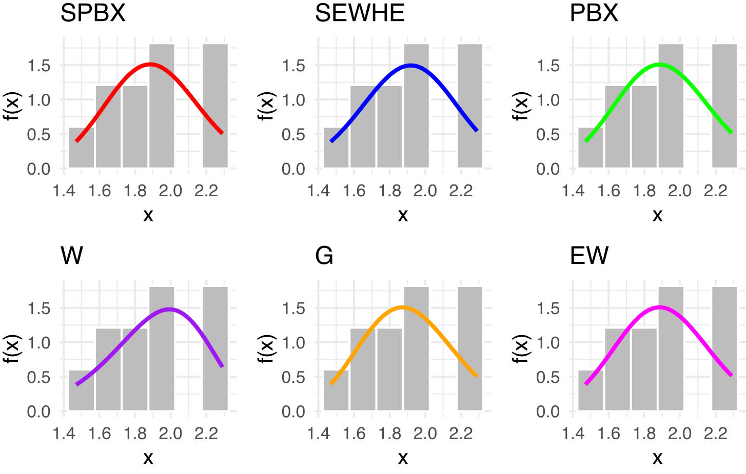
Our analysis focused on the latitude data from two key regions, the Southwest and East. The latitude values for the Southwest region are: 1.47, 1.63, 1.63, 1.76, 1.87, 1.88, 1.92, 2.02, 2.25, 2.27, 2.29, and for the east region: 2.45, 2.59, 3.17, 3.56, 3.78, 3.90, 4.23, 4.76, 4.94, 5.32, 5.97, 6.17. In Tables 10 and 11, we provide an in-depth comparison of various models using MLE with StEr, KSD, PVKS, CVM, PVCVM, AD, and PVAD. Among the tested distributions, the SPB-X distribution consistently outperformed others across multiple metrics, including KSD, PVKS, CVM, PVCVM, AD, and PVAD, making it the most suitable model for this rainfall dataset.
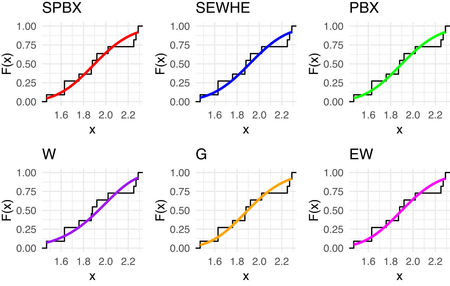
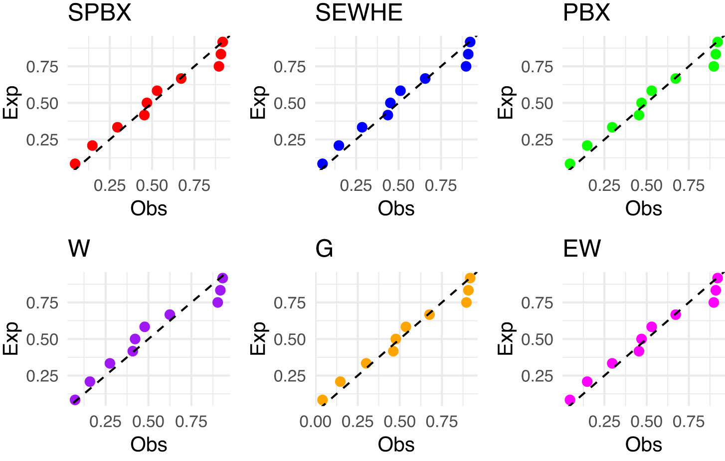
Figures 4 and 5 includes the histogram, violin plot, QQ (quantile-quantile) plot, box plot with stripchart, and TTT (total time in test) plot of dataset of rain gauge stations datasets. The estimated PDFs of competing models for the datasets of rain gauge stations datasets are shown in Figures 6 and 9, while Figures 7 and 10 display the estimated CDFs of the competitive models. Furthermore, Figures 8 and 11 illustrate the PP plots of the competing models. Figures 6–11 demonstrate the fit of our distribution to the actual data.
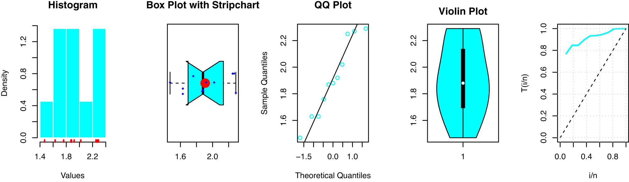
Some basic nonparametric plots for latitude for southwest of rain gauge stations.
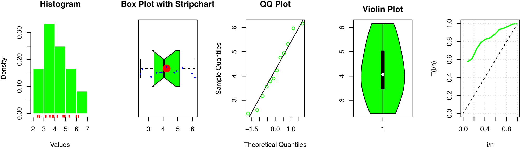
Some basic nonparametric plots for latitude for west of rain gauge stations.
Estimated PDFs for the competing models for latitude for southwest of rain gauge stations.
Estimated CDFs for the competing models for latitude for southwest of rain gauge stations.
The PP plot for the competing models for latitude for southwest of rain gauge stations.
Estimated PDFs for the competing models for latitude for west of rain gauge stations.
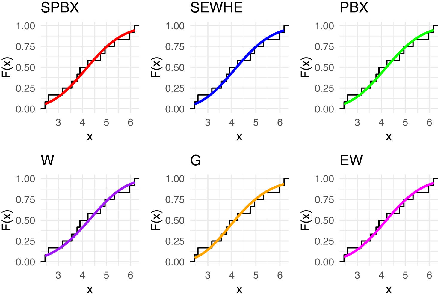
Estimated CDFs for the competing models for latitude for west of rain gauge stations.

The PP plot for the competing models for latitude for west of rain gauge stations.
8.2 Breaking stress of carbon fibers dataset
The breaking stress of carbon fibers dataset contains crucial measurements of the maximum stress that carbon fibers can endure before fracturing. This dataset is indispensable for researchers and engineers in the fields of materials science and engineering. It plays a key role in investigating the mechanical properties and performance of carbon fiber-reinforced composites, widely used in industries such as aerospace and automotive manufacturing.
As mentioned by Cordeiro and Lemonte [40], this specific dataset offers valuable insights into the behavior of carbon fibers under stress. Below is the dataset:
{3.15, 1.25, 2.95, 4.38, 2.12, 1.47, 0.39, 2.79, 2.59, 2.05, 2.56, 3.65, 2.74, 1.87, 3.56, 4.42, 3.31, 2.55, 2.03, 3.19, 2.67, 3.22, 2.48, 2.43, 4.70, 3.09, 4.90, 1.61, 3.22, 2.50, 2.93, 3.68, 1.57, 1.80, 2.53, 2.81, 1.84, 2.87, 1.61, 3.11, 2.41, 3.60, 3.75, 3.27, 2.82, 2.35, 2.96, 3.39, 2.55, 0.85, 3.28, 3.11, 2.03, 1.08, 3.27, 2.03, 1.69, 3.39, 2.73, 3.31, 2.88, 4.20, 3.33}.
This dataset allows for deeper analysis into the variability and resilience of carbon fibers under extreme stress conditions. Researchers can apply these data to optimize material performance and design more efficient and durable composites, which are integral to high-stress environments.
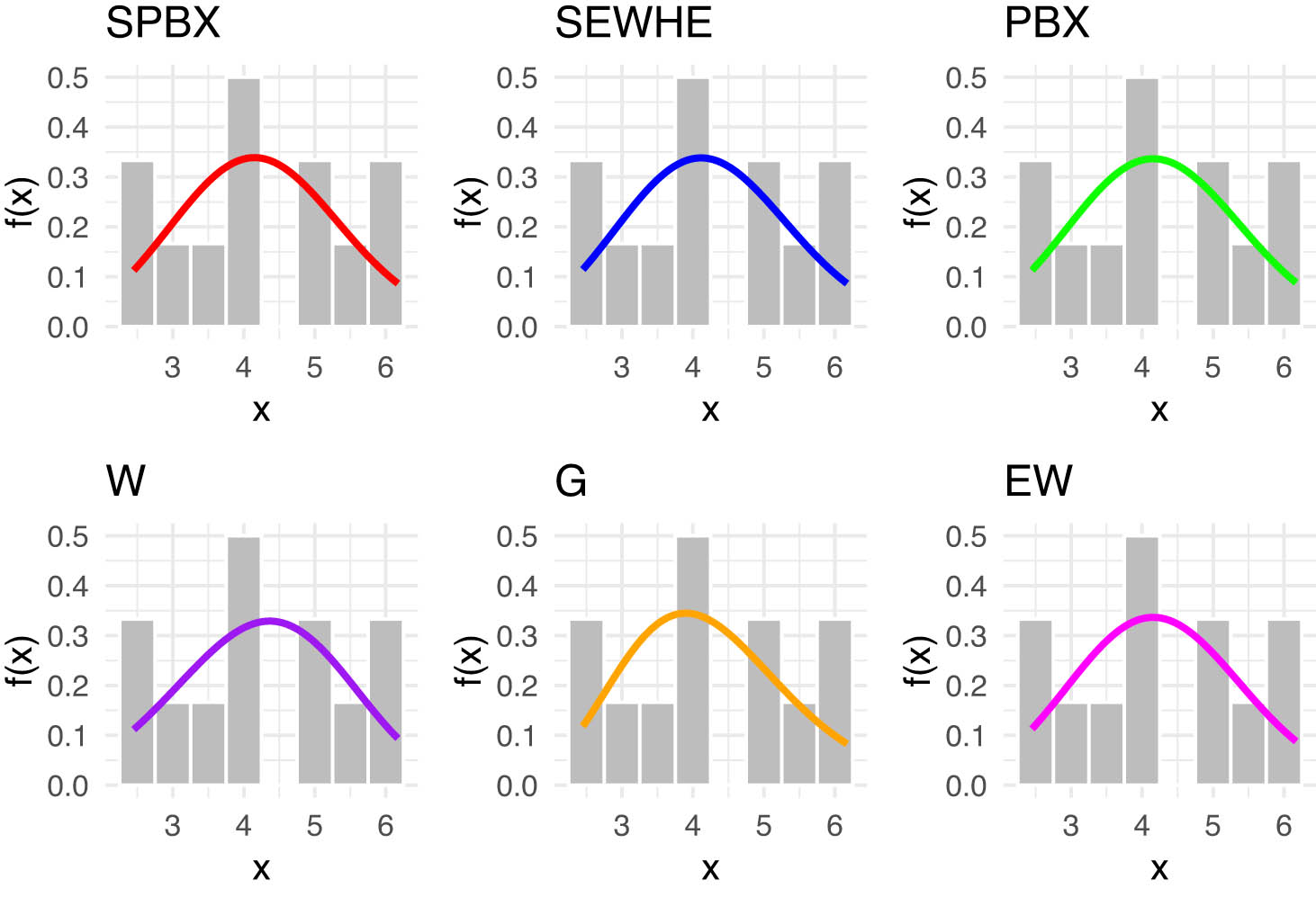
In Table 12, we provide an in-depth comparison of various models using MLE with StEr, KSD, PVKS, CVM, PVCVM, AD, and PVAD. Among the tested distributions, the SPB-X distribution consistently outperformed others across multiple metrics, including KSD, PVKS, CVM, PVCVM, AD, and PVAD, making it the most suitable model for breaking stress of carbon fibers dataset.
Figure 12 includes the histogram, violin plot, QQ plot, box plot with stripchart, and TTT plot of dataset of breaking stress of carbon fibers datasets. The estimated PDFs of competing models for the of dataset of breaking stress of carbon fibers datasets are shown in Figure 13, while Figure 14 displays the estimated CDFs of the competitive models. In addition, Figure 15 illustrates the PP plots of the competing models. Figures 13–15 demonstrate the fit of our distribution to the actual data.

Some basic nonparametric plots for dataset of carbon fibers stress.
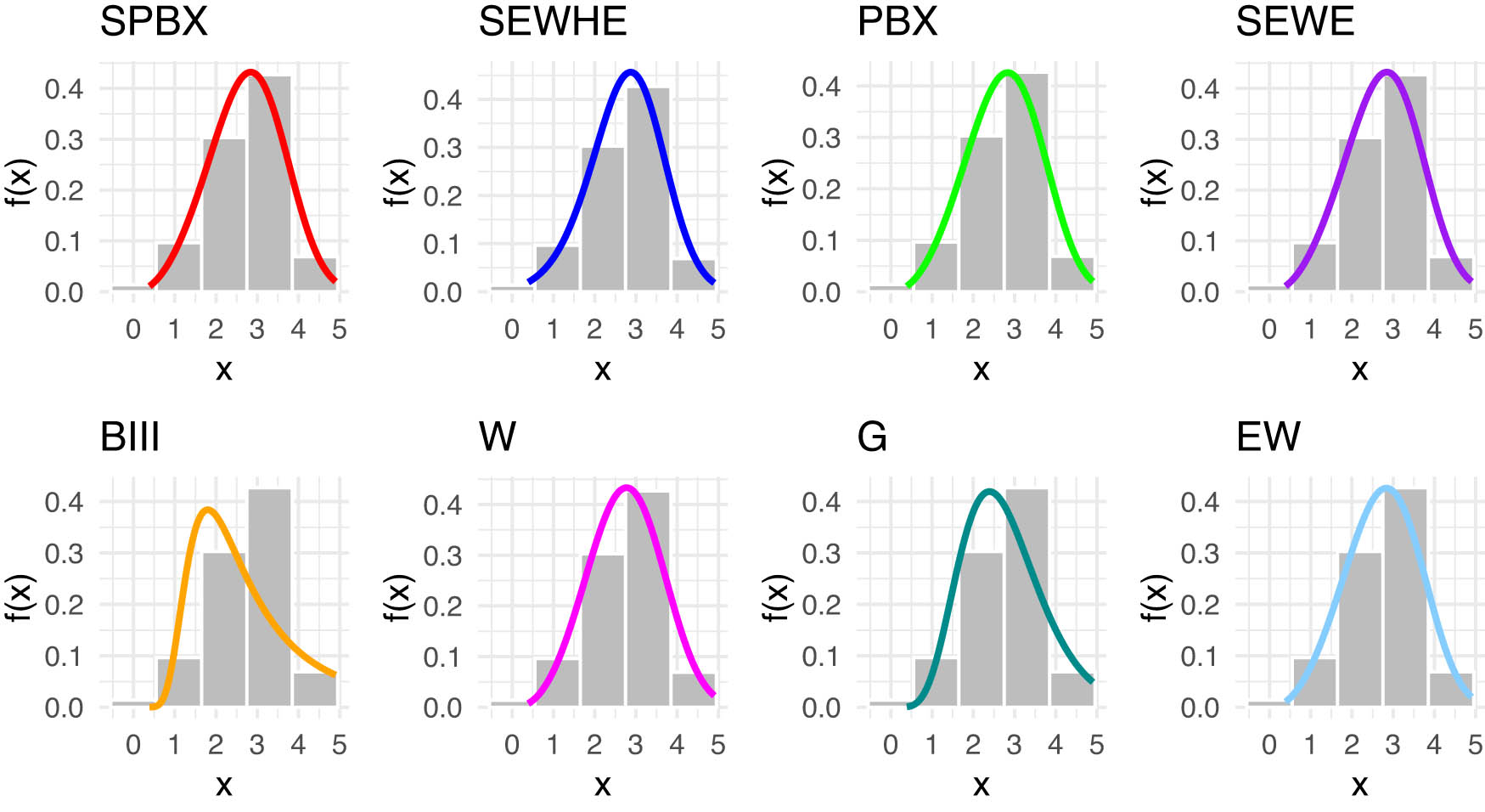
Estimated PDFs for the competing models for dataset of carbon fibers stress.
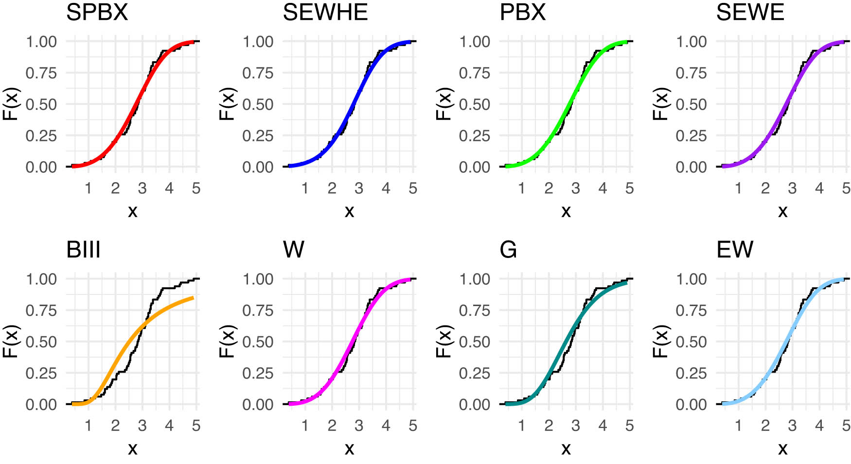
Estimated CDFs for the competing models for dataset of carbon fibers stress.
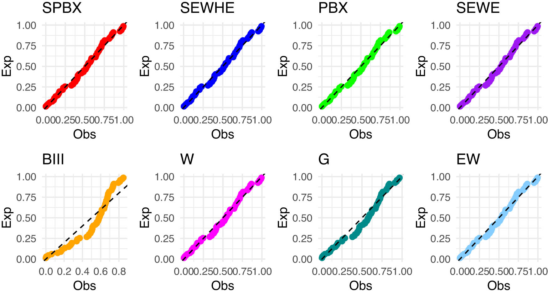
The PP plot for the competing models for dataset of carbon fibers stress.
8.3 Tensile strength of carbon fibers dataset
Tensile strength, typically expressed in Gigapascals (GPa), measures the maximum stress a single carbon fiber can withstand before fracturing under tension. This property is essential in evaluating the performance and reliability of carbon fiber-reinforced materials, widely applied across industries such as aerospace, automotive, and sports equipment manufacturing. An in-depth understanding of the tensile strength of carbon fibers directly influences the design and development of more durable and resilient composite structures.
The dataset used in this study, sourced from Kundu and Raqab [41], contains tensile strength measurements for individual carbon fibers, expressed in GPa. The following is the dataset:
{1.098, 1.253, 0.944, 1.055, 1.586, 1.773, 1.554, 2.012, 1.301, 1.179, 1.884, 0.966, 0.552, 1.179, 1.642, 0.312, 1.426, 1.726, 0.865, 1.063, 0.803, 1.514, 1.270, 2.233, 1.301, 1.240, 1.627, 2.096, 1.533, 1.534, 1.321, 1.801, 1.559, 0.865, 0.979, 2.094, 1.300, 0.865, 1.434, 1.235, 2.585, 1.684, 2.012, 1.048, 1.373, 1.633, 1.697, 0.753, 1.726, 1.754}.
This dataset provides critical insights into the variability of tensile strength between individual fibers, allowing engineers and materials scientists to optimize the use of carbon fibers in high-performance applications. Using such data, industries can create composites that push the boundaries of durability and functionality in demanding environments.
In Table 13, we provide an in-depth comparison of various models using MLE with StEr, KSD, PVKS, CVM, PVCVM, AD, and PVAD. Among the tested distributions, the SPB-X distribution consistently outperformed others across multiple metrics, including KSD, PVKS, CVM, PVCVM, AD, and PVAD, making it the most suitable model for the tensile strength of the carbon fibers dataset.
Figure 16 includes the histogram, violin plot, QQ plot, box plot with stripchart, and TTT plot of dataset of tensile stress of carbon fibers datasets. The estimated PDFs of competing models for the of dataset of tensile stress of carbon fibers datasets are shown in Figure 17, while Figure 18 displays the estimated CDFs of the competitive models. In addition, Figure 19 illustrates the PP plots of the competing models. Figures 17–19 demonstrate the fit of our distribution to the actual data.

Some basic nonparametric plots for dataset of carbon fibers strength.

The PDF plot of SPB-X distribution for dataset of carbon fibers strength.

The CDF plot of SPB-X distribution for dataset of carbon fibers strength.
The PP plot of SPB-X distribution for dataset of carbon fibers strength.
8.4 Insurance dataset
The insurance dataset, which spans the years 1987–2017, displays the excess of assets over liabilities for investments made by insurance companies, pension funds, and trusts. The values are expressed in billions of pounds. The following is the electronic address that it was obtained from: The link https://www.ons.gov.uk/ references the aforementioned product. The dataset is reported in Table 14.
Sed Excess of assets over liabilities for investment by insurance companies, and pension funds
| Period | Value | Period | Value | Period | Value |
|---|---|---|---|---|---|
| 1986 | 2.151 | 1997 | 4.301 | 2008 | 15.264 |
| 1987 | 2.208 | 1998 | 8.421 | 2009 | 4.547 |
| 1988 | 2.170 | 1999 | 6.661 | 2010 | 3.261 |
| 1989 | 2.707 | 2000 | 6.548 | 2011 | 3.426 |
| 1990 | 2.014 | 2001 | 4.977 | 2012 | 6.418 |
| 1991 | 1.698 | 2002 | 4.202 | 2013 | 7.389 |
| 1992 | 2.512 | 2003 | 5.580 | 2014 | 6.136 |
| 1993 | 4.857 | 2004 | 8.856 | 2015 | 5.820 |
| 1994 | 3.509 | 2005 | 6.902 | 2016 | 3.094 |
| 1995 | 5.066 | 2006 | 5.442 | 2017 | 8.216 |
| 1996 | 5.413 | 2007 | 8.067 |
In Table 15, we provide an in-depth comparison of various models using MLE with StEr, KSD, PVKS, CVM, PVCVM, AD, and PVAD. Among the tested distributions, the SPB-X distribution consistently outperformed others across multiple metrics, including KSD, PVKS, CVM, PVCVM, AD, and PVAD, making it the most suitable model for insurance dataset.
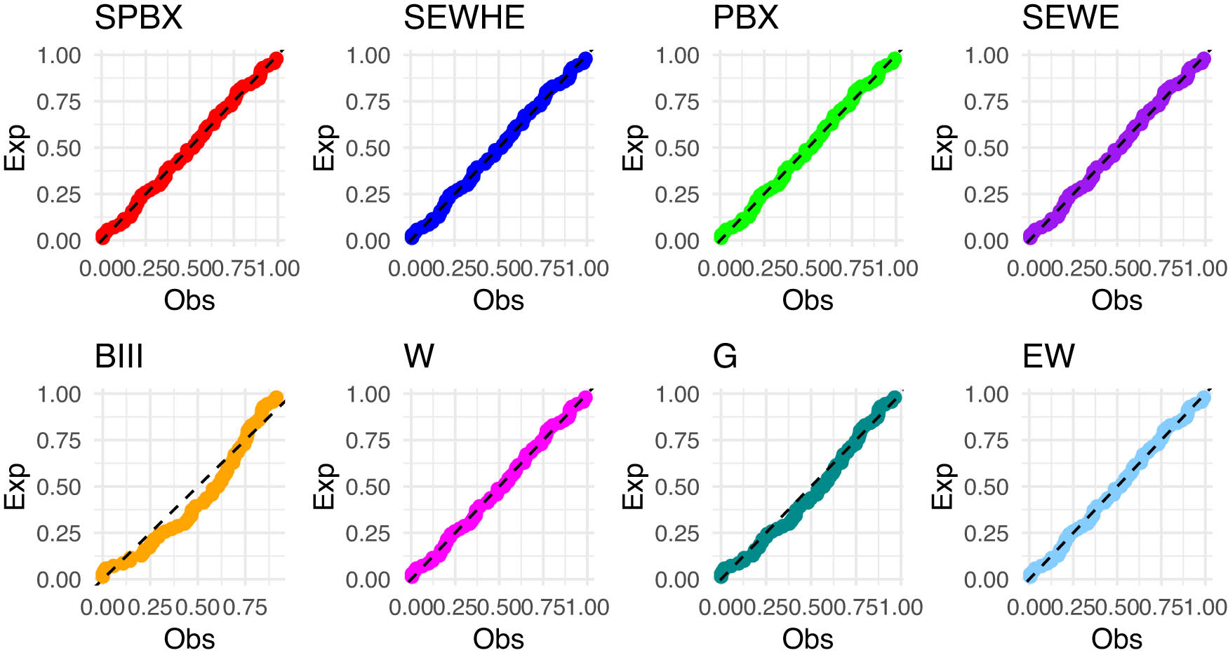
Figure 20 includes the histogram, violin plot, QQ plot, box plot with stripchart, and TTT plot of dataset of insurance datasets. The estimated PDFs of competing models for the of dataset of insurance datasets are shown in Figure 21, while Figure 22 displays the estimated CDFs of the competitive models. In addition, Figure 23 illustrates the PP plots of the competing models. Figures 21–23 demonstrate the fit of our distribution to the actual data.

Some basic nonparametric plots for insurance dataset.
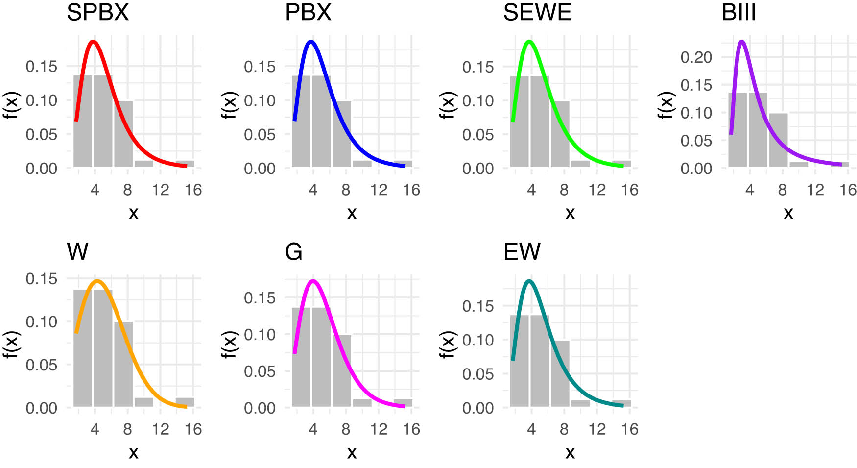
Estimated PDFs for the competing models for insurance dataset.
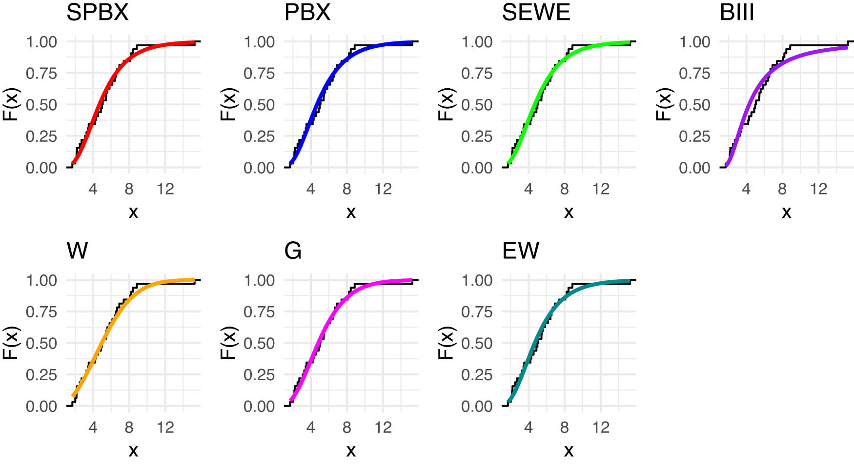
Estimated CDFs for the competing models for insurance dataset.

Estimated CDFs for the competing models for insurance dataset.
The actuarial measures VaR, ES, TVaR, TV, and TVP of the SPB-X, PBX, and SEWE distributions are computed and compared using the actual dataset in the following. Tables 16 and 17 present the numerical findings.
The actuarial metrics VaR, ES, TVaR, and TV values for the insurance dataset
| Measure |
|
SPB-X | PBX | SEWE | Measure |
|
SPB-X | PBX | SEWE |
|---|---|---|---|---|---|---|---|---|---|
| VaR | 0.650 | 5.6930 | 5.6868 | 5.6815 | TVaR | 0.650 | 8.1786 | 8.1798 | 8.1864 |
| 0.700 | 6.0936 | 6.0942 | 6.0883 | 0.700 | 8.5602 | 8.5620 | 8.5707 | ||
| 0.750 | 6.5548 | 6.5636 | 6.5577 | 0.750 | 9.0087 | 9.0100 | 9.0215 | ||
| 0.800 | 7.1068 | 7.1253 | 7.1199 | 0.800 | 9.5554 | 9.5537 | 9.5695 | ||
| 0.850 | 7.8061 | 7.8351 | 7.8317 | 0.850 | 10.2603 | 10.2501 | 10.2728 | ||
| 0.900 | 8.7813 | 8.8196 | 8.8215 | 0.900 | 11.2598 | 11.2275 | 11.2621 | ||
| 0.910 | 9.0343 | 9.0736 | 9.0772 | 0.910 | 11.5214 | 11.4812 | 11.5193 | ||
| 0.920 | 9.3174 | 9.3569 | 9.3629 | 0.920 | 11.8150 | 11.7648 | 11.8070 | ||
| 0.930 | 9.6388 | 9.6776 | 9.6864 | 0.930 | 12.1493 | 12.0863 | 12.1336 | ||
| 0.940 | 10.0109 | 10.0474 | 10.0598 | 0.940 | 12.5376 | 12.4578 | 12.5112 | ||
| 0.950 | 10.4529 | 10.4843 | 10.5016 | 0.950 | 13.0001 | 12.8975 | 12.9586 | ||
| 0.960 | 10.9973 | 11.0190 | 11.0430 | 0.960 | 13.5715 | 13.4364 | 13.5076 | ||
| 0.970 | 11.7060 | 11.7088 | 11.7426 | 0.970 | 14.3173 | 14.1328 | 14.2184 | ||
| 0.975 | 12.1596 | 12.1465 | 12.1873 | 0.975 | 14.7957 | 14.5752 | 14.6705 | ||
| 0.980 | 12.7200 | 12.6832 | 12.7331 | 0.980 | 15.3873 | 15.1177 | 15.2255 | ||
| 0.985 | 13.4515 | 13.3766 | 13.4396 | 0.985 | 16.1607 | 15.8193 | 15.9443 | ||
| 0.990 | 14.5011 | 14.3577 | 14.4412 | 0.990 | 17.2715 | 16.8120 | 16.9634 | ||
| 0.995 | 16.3499 | 16.0457 | 16.1700 | 0.995 | 19.2293 | 18.5203 | 18.7222 | ||
| 0.999 | 20.9308 | 20.0204 | 20.2655 | 0.999 | 24.0749 | 22.5402 | 22.8827 | ||
| ES | 0.650 | 3.6882 | 3.6717 | 3.0239 | TV | 0.650 | 6.2552 | 5.9357 | 6.0739 |
| 0.700 | 3.8454 | 3.8299 | 3.1817 | 0.700 | 6.2759 | 5.9001 | 6.0496 | ||
| 0.750 | 4.0103 | 3.9961 | 3.3478 | 0.750 | 6.3207 | 5.8717 | 6.0364 | ||
| 0.800 | 4.1860 | 4.1735 | 3.5252 | 0.800 | 6.4003 | 5.8557 | 6.0379 | ||
| 0.850 | 4.3774 | 4.3671 | 3.7190 | 0.850 | 6.5323 | 5.8534 | 6.0582 | ||
| 0.900 | 4.5932 | 4.5853 | 3.9378 | 0.900 | 6.7623 | 5.8743 | 6.1107 | ||
| 0.910 | 4.6406 | 4.6332 | 3.9859 | 0.910 | 6.8288 | 5.8828 | 6.1274 | ||
| 0.920 | 4.6898 | 4.6830 | 4.0359 | 0.920 | 6.9061 | 5.8936 | 6.1473 | ||
| 0.930 | 4.7413 | 4.7350 | 4.0881 | 0.930 | 6.9969 | 5.9070 | 6.1710 | ||
| 0.940 | 4.7953 | 4.7895 | 4.1429 | 0.940 | 7.1061 | 5.9239 | 6.1998 | ||
| 0.950 | 4.8525 | 4.8470 | 4.2009 | 0.950 | 7.2404 | 5.9453 | 6.2352 | ||
| 0.960 | 4.9135 | 4.9084 | 4.2628 | 0.960 | 7.4118 | 5.9739 | 6.2815 | ||
| 0.970 | 4.9797 | 4.9748 | 4.3299 | 0.970 | 7.6437 | 6.0116 | 6.3398 | ||
| 0.975 | 5.0153 | 5.0104 | 4.3660 | 0.975 | 7.7954 | 6.0358 | 6.3776 | ||
| 0.980 | 5.0532 | 5.0482 | 4.4043 | 0.980 | 8.1037 | 6.0678 | 6.4260 | ||
| 0.985 | 5.0938 | 5.0886 | 4.4454 | 0.985 | 8.2437 | 6.1081 | 6.4876 | ||
| 0.990 | 5.1385 | 5.1328 | 4.4906 | 0.990 | 8.6181 | 6.1666 | 6.5745 | ||
| 0.995 | 5.1897 | 5.1829 | 4.5421 | 0.995 | 9.2927 | 6.2645 | 6.7159 | ||
| 0.999 | 5.2410 | 5.2322 | 4.5935 | 0.999 | 10.9996 | 6.4753 | 7.0392 |
The actuarial metrics TVP values for the insurance dataset
|
|
|
SPB-X | PBX | SEWE |
|
|
SPB-X | PBX | SEWE |
|---|---|---|---|---|---|---|---|---|---|
| 0.50 | 0.650 | 11.3062 | 11.1476 | 11.2233 | 0.90 | 0.650 | 13.8083 | 13.5219 | 13.6528 |
| 0.700 | 11.6982 | 11.5121 | 11.5955 | 0.700 | 14.2085 | 13.8721 | 14.0153 | ||
| 0.750 | 12.1690 | 11.9459 | 12.0397 | 0.750 | 14.6973 | 14.2946 | 14.4543 | ||
| 0.800 | 12.7555 | 12.4815 | 12.5884 | 0.800 | 15.3156 | 14.8238 | 15.0036 | ||
| 0.850 | 13.5265 | 13.1768 | 13.3019 | 0.850 | 16.1395 | 15.5182 | 15.7251 | ||
| 0.900 | 14.6410 | 14.1646 | 14.3174 | 0.900 | 17.3459 | 16.5143 | 16.7617 | ||
| 0.910 | 14.9358 | 14.4226 | 14.5830 | 0.910 | 17.6674 | 16.7757 | 17.0340 | ||
| 0.920 | 15.2680 | 14.7116 | 14.8807 | 0.920 | 18.0304 | 17.0690 | 17.3396 | ||
| 0.930 | 15.6478 | 15.0398 | 15.2191 | 0.930 | 18.4466 | 17.4026 | 17.6875 | ||
| 0.940 | 16.0906 | 15.4197 | 15.6110 | 0.940 | 18.9331 | 17.7893 | 18.0910 | ||
| 0.950 | 16.6203 | 15.8702 | 16.0762 | 0.950 | 19.5165 | 18.2483 | 18.5702 | ||
| 0.960 | 17.2774 | 16.4234 | 16.6484 | 0.960 | 20.2421 | 18.8129 | 19.1610 | ||
| 0.970 | 18.1391 | 17.1386 | 17.3882 | 0.970 | 21.1966 | 19.5432 | 19.9242 | ||
| 0.975 | 18.6934 | 17.5931 | 17.8593 | 0.975 | 21.8115 | 20.0074 | 20.4103 | ||
| 0.980 | 19.4391 | 18.1517 | 18.4385 | 0.980 | 22.6806 | 20.5788 | 21.0089 | ||
| 0.985 | 20.2825 | 18.8733 | 19.1881 | 0.985 | 23.5800 | 21.3166 | 21.7831 | ||
| 0.990 | 21.5805 | 19.8953 | 20.2507 | 0.990 | 25.0278 | 22.3620 | 22.8805 | ||
| 0.995 | 23.8756 | 21.6525 | 22.0802 | 0.995 | 27.5927 | 24.1583 | 24.7666 | ||
| 0.999 | 29.5747 | 25.7779 | 26.4023 | 0.999 | 33.9745 | 28.3680 | 29.2180 | ||
| 0.75 | 0.650 | 12.8700 | 12.6316 | 12.7418 | 0.99 | 0.650 | 14.3712 | 14.0561 | 14.1995 |
| 0.700 | 13.2672 | 12.9871 | 13.1079 | 0.700 | 14.7734 | 14.4031 | 14.5598 | ||
| 0.750 | 13.7492 | 13.4138 | 13.5488 | 0.750 | 15.2661 | 14.8230 | 14.9976 | ||
| 0.800 | 14.3556 | 13.9454 | 14.0979 | 0.800 | 15.8916 | 15.3508 | 15.5470 | ||
| 0.850 | 15.1596 | 14.6402 | 14.8164 | 0.850 | 16.7274 | 16.0450 | 16.2704 | ||
| 0.900 | 16.3316 | 15.6332 | 15.8451 | 0.900 | 17.9545 | 17.0430 | 17.3116 | ||
| 0.910 | 16.6431 | 15.8933 | 16.1149 | 0.910 | 18.2820 | 17.3052 | 17.5855 | ||
| 0.920 | 16.9945 | 16.1850 | 16.4175 | 0.920 | 18.6520 | 17.5994 | 17.8929 | ||
| 0.930 | 17.3970 | 16.5166 | 16.7619 | 0.930 | 19.0763 | 17.9343 | 18.2429 | ||
| 0.940 | 17.8672 | 16.9007 | 17.1610 | 0.940 | 19.5726 | 18.3224 | 18.6489 | ||
| 0.950 | 18.4304 | 17.3565 | 17.6350 | 0.950 | 20.1681 | 18.7834 | 19.1314 | ||
| 0.960 | 19.1304 | 17.9168 | 18.2187 | 0.960 | 20.9092 | 19.3506 | 19.7263 | ||
| 0.970 | 20.0500 | 18.6415 | 18.9732 | 0.970 | 21.8845 | 20.0843 | 20.4947 | ||
| 0.975 | 20.6422 | 19.1020 | 19.4537 | 0.975 | 22.5131 | 20.5506 | 20.9843 | ||
| 0.980 | 21.4650 | 19.6686 | 20.0450 | 0.980 | 23.4099 | 21.1249 | 21.5873 | ||
| 0.985 | 22.3434 | 20.4004 | 20.8100 | 0.985 | 24.3219 | 21.8663 | 22.3670 | ||
| 0.990 | 23.7351 | 21.4370 | 21.8943 | 0.990 | 25.8034 | 22.9170 | 23.4722 | ||
| 0.995 | 26.1988 | 23.2187 | 23.7592 | 0.995 | 28.4290 | 24.7221 | 25.3710 | ||
| 0.999 | 32.3246 | 27.3967 | 28.1621 | 0.999 | 34.9645 | 28.9508 | 29.8515 |
Figure 24 includes the competing model VaR, ES, TVaR, and TV plots for the insurance dataset. the competing model TVP plots for the insurance dataset shown in Figure 25.
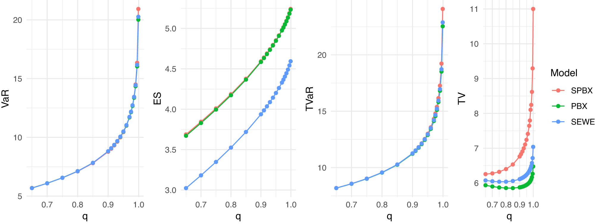
Competing model VaR, ES, TVaR, and TV plots for the insurance dataset.
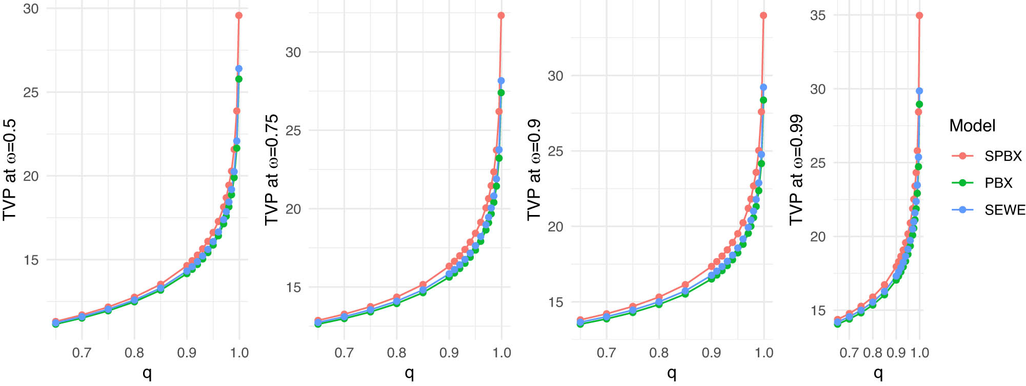
Competing model TVP plots for the insurance dataset.
We find that for different significance levels
From Table 18, it is observed that both estimation methods produce consistent results with only minor differences in the estimated parameters. In several datasets (Data1, Data3, Data4, and Data5), LSE achieves slightly smaller KS values and higher
Parameter estimates of the SPB-X distribution using MLE and LSE for the five datasets, along with KSD and PVKS
| Data | Method |
|
|
|
KSD | PVKS |
|---|---|---|---|---|---|---|
| Data1 | MLE | 14.5195 | 0.8207 | 1.0578 | 0.1684 | 0.9141 |
| LSE | 19.8840 | 1.0673 | 0.7378 | 0.1415 | 0.9803 | |
| Data2 | MLE | 2.7126 | 0.2305 | 1.0543 | 0.1036 | 0.9978 |
| LSE | 1.7772 | 0.1973 | 1.0428 | 0.1088 | 0.9957 | |
| Data3 | MLE | 0.8472 | 0.0878 | 1.8287 | 0.0784 | 0.8124 |
| LSE | 0.5967 | 0.0255 | 2.7033 | 0.0616 | 0.9635 | |
| Data4 | MLE | 0.8548 | 0.2995 | 1.7155 | 0.0470 | 0.9980 |
| LSE | 1.0035 | 0.3514 | 1.5885 | 0.0386 | 0.9999 | |
| Data5 | MLE | 16.8042 | 1.0771 | 0.2799 | 0.0881 | 0.9463 |
| LSE | 0.6613 | 0.0505 | 1.3798 | 0.0791 | 0.9787 |
9 Concluding remarks
In this article, we discuss a novel three-parameter lifespan distribution known as the sine power Burr X (SPB-X) distribution. The suggested distribution is derived from the sine-G class of distributions and the power Burr-X distribution. The suggested distribution encompasses several features, including explicit formulations for the quantile function, Bowley skewness, Moors kurtosis, ordinary moments, generating function, and incomplete and conditional moments, with several numerical and graphical representations. Several notable reliability measures for the SPB-X model include standard reliability functions, mean residual life function, mean waiting time function, residual moment, and inverted residual life. Several critical risk metrics for the SPB-X distribution. Risk measurements include the value at risk, projected shortfall, TVaR, TV, and TVP. Four estimation strategies were used to determine the model parameters: maximum likelihood, least squares, MPS, and Bayesian. A simulation study is conducted to evaluate the efficacy of estimating techniques. Ultimately, five actual datasets are examined to assess the utility and adaptability of the suggested approach. The limitation of this article lies in estimating the parameters of the SPB-X model using the complete samples only. This reason opens the door for future studies to study the estimation of the parameters of the new distribution using different censored schemes for the censored data.
-
Funding information: This work was supported and funded by the Deanship of Scientific Research at Imam Mohammad Ibn Saud Islamic University (IMSIU) (grant number IMSIU-DDRSP2502).
-
Author contribution: All authors have accepted responsibility for the entire content of this manuscript and approved its submission.
-
Conflict of interest: The authors state no conflict of interest.
-
Data availability statement: The data that support the findings of this study are available on request from the corresponding author. The data are not publicly available due to privacy or ethical restrictions.
References
[1] Eugene N, Lee C, Famoye F. Beta-normal distribution and its applications. Commun Stat Theory Methods. 2002;31(4):497–512. 10.1081/STA-120003130Search in Google Scholar
[2] Cordeiro GM, de Castro M. A new family of generalized distributions. J Stat Comput Simulat. 2011;81(7):883–98. 10.1080/00949650903530745Search in Google Scholar
[3] Alzaatreh A, Lee C, Famoye F. A new method for generating families of continuous distributions. Metron. 2013;71:63–79. 10.1007/s40300-013-0007-ySearch in Google Scholar
[4] Hassan AS, Elgarhy M, Shakil M. Type II half-Logistic family of distributions with applications. Pakistan J Stat Operat Res. 2017;13(2):245–64. 10.18187/pjsor.v13i2.1560Search in Google Scholar
[5] Al-Marzouki S, Jamal F, Chesneau Ch, Elgarhy M. Topp-Leone odd Fréchet generated family of distributions with applications to COVID-19 data sets. Comput Model Eng Sci. 2020;125(1):437–58. 10.32604/cmes.2020.011521Search in Google Scholar
[6] Kumar D, Singh U, Singh SK. A new distribution using sine function its application to bladder cancer patients data. J Stat Appl Pro. 2015;4(3):417–27. Search in Google Scholar
[7] Souza L, Junior WRO, de Brito CCR, Chesneau C, Ferreira TAE, Soares L. Generalproperties for the Cos-G class of distributions with applications. Eurasian Bull Math. 2019;2:63–79. Search in Google Scholar
[8] Chesneau C, Jamal F The sine Kumaraswamy-G family of distributions. J Math Ext. 2021;15:1–33. Search in Google Scholar
[9] Al-Babtain AA, Elbatal I, Chesneau C, Elgarhy M. Sine Topp-Leone-G family of distributions: theory and applications. Open Phys. 2020;18:574–93. 10.1515/phys-2020-0180Search in Google Scholar
[10] Souza L, Junior WRO, de Brito CCR, Chesneau C, Ferreira TAE, Fernandes LR. Tan-G class of trigonometric distributions and its applications. Cubo. 2021;23:1–20. 10.4067/S0719-06462021000100001Search in Google Scholar
[11] Wenjing H, Afify Z, Goual H. The arcsine exponentiated-X family: validation andinsurance application. Complexity. 2020;2020:1–18. 10.1155/2020/8394815Search in Google Scholar
[12] Burr IW. Cumulative frequency functions. Ann Math Stat. 1942;13(2):215–32. 10.1214/aoms/1177731607Search in Google Scholar
[13] Raqab MZ, Kundu D. Burr type X distribution: Revisited. J Probabil Stat Sci. 2006;4:179–93. Search in Google Scholar
[14] Surles JG, Padgett WJ. Inference for reliability and stress-strength for a scaled Burr type X distribution. Lifetime Data Anal. 2001;7:187–200. 10.1023/A:1011352923990Search in Google Scholar PubMed
[15] Algarni A, Almarashi AM, Elbatal I, Hassan AS, Almetwally EM, Daghistani AM, et al. Type I half logistic Burr XG family: Properties, Bayesian, and non-Bayesian estimation under censored samples and applications to COVID-19 data. Math Problems Eng. 2021;2021:5461130. 10.1155/2021/5461130Search in Google Scholar
[16] Abonongo J, Mwaniki IJ, Aduda JA. Cosine Fréchet loss distribution: properties, actuarial measures and insurance applications. Comput J Math Stat Sci. 2024;3(1):1–32. 10.21608/cjmss.2023.240185.1019Search in Google Scholar
[17] Bantan RAR, Chesneau C, Jamal F, Elbatal I, Elgarhy M. The truncated Burr X-G family of distributions: Properties and applications to actuarial and financial data. Entropy 2021;23:1088. 10.3390/e23081088Search in Google Scholar PubMed PubMed Central
[18] Suleiman AA, Daud H, Singh NSS, Ishaq AI, Othman M. A new odd beta prime-Burr X distribution with applications to petroleum rock sample data and COVID-19 mortality rate. Data. 2023;8:143. 10.3390/data8090143Search in Google Scholar
[19] Soliman D, Hegazy MA, AL-Dayian GR, EL-Helbawy AA. Statistical properties and applications of a new truncated Zubair-generalized family of distributions. Comput J Math Stat Sci. 2025;4(1):222–57. 10.21608/cjmss.2024.322714.1073Search in Google Scholar
[20] Khan MS, King R, Hudson IL. Transmuted Burr type X distribution with covariates regression modeling to analyze reliability data. Am J Math Manag Sci. 2020;39:99–121. 10.1080/01966324.2019.1605320Search in Google Scholar
[21] Elbatal IA, Helal TS, Elsehetry AM, Elshaarawy RS. Topp-Leone Weibull generated family of distributions with applications. J Business Environ Sci. 2022;1(1):183–95. 10.21608/jcese.2022.270143. Search in Google Scholar
[22] Usman RM, Ilyas M. The power Burr Type X distribution: Properties, regression modeling and applications. Punjab Univ J Math. 2020;52:27–44. Search in Google Scholar
[23] Butt NS, Khalil MG. A new bimodal distribution for modeling asymmetric bimodal heavy- tail real lifetime data. Symmetry. 2020;12:2058. 10.3390/sym12122058Search in Google Scholar
[24] Usman RM, Handique L, Chakraborty S. Some aspects of the odd log-logistic Burr X distribution with applications in reliability data modeling. Int J Appl Math Stat. 2019;58:127–47. Search in Google Scholar
[25] Shrahili M, Elbatal M, Muhammad M. The type I half-logistic Burr X distribution: Theory and practice. J Nonlinear Sci Appl 2019;12:262–77. 10.22436/jnsa.012.05.01Search in Google Scholar
[26] Abdullah ZM, Khaleel MA, Abdal-hameed MK, Oguntunde PE. Estimating parameters for extension of Burr type X distribution by using conjugate gradient in unconstrained optimization. Kirkuk Univ. 2019;14:33–49. 10.32894/kujss.2019.14.3.4Search in Google Scholar
[27] Khaleel MA, Ibrahim NA, Shitan M, Merovci F. New extension of Burr type X distribution properties with application. J King Saud Univ Sci. 2018;30(4):450–7. 10.1016/j.jksus.2017.05.007Search in Google Scholar
[28] Madaki UY, Abu Bakar MR, Handique L. Beta Kumaraswamy Burr type X distribution and its properties. Preprints 2018;2018080356. 10.20944/preprints201808.0356.v1Search in Google Scholar
[29] Ishaq A, Usman A, Tasi’u M, Aliyu Y. Weibull-Burr type x distribution: Its properties and application. Niger. 2017;16:150–7. Search in Google Scholar
[30] Al-Saiari AY, Baharith LA, Mousa SA. New extended burr type X distribution. Sri Lankan J Appl Stat. 2016;17:217–31. 10.4038/sljastats.v17i3.7904Search in Google Scholar
[31] Khaleel MA, Ibrahim NA, Shitan M, Merovci F. Some properties of Gamma Burr type X distribution with application. In Proceedings of the AIP Conference Proceedings, Yogyakarta, Indonesia, 25–26 January 2016; p. 020087. 10.1063/1.4952567Search in Google Scholar
[32] Merovci F, Khaleel MA, Ibrahim NA, Shitan M. The beta Burr type X distribution properties with application. SpringerPlus. 2016;5:697. 10.1186/s40064-016-2271-9Search in Google Scholar PubMed PubMed Central
[33] Hassan OHM, Elbatal I, Al-Nefaie AH, Elgarhy M. On the Kavya-Manoharan-Burr X model: estimations under ranked set sampling and applications. J Risk Financial Manag. 2023;16:19. 10.3390/jrfm16010019Search in Google Scholar
[34] Kenney FJ, Keeping SE. Mathematics of statistics. NJ: Princeton; 1962. Search in Google Scholar
[35] Moors AJ. A quantile alternative for Kurtosis. J R Stat Soc D. 1998;37:25–32. 10.2307/2348376Search in Google Scholar
[36] Artzner P. Application of coherent risk measures to capital requirements in insurance. North Am Actuarial J. 1999;3(2):11–25. 10.1080/10920277.1999.10595795Search in Google Scholar
[37] Artzner P, Delbaen F, Eber J-M, Heath D. Thinking coherently. Risk. 1997;10(11):14. Search in Google Scholar
[38] Artzner P, Delbaen F, Eber J-M, Heath D. Coherent measures of risk. Math Fin. 1999;9(3):203–28. 10.1111/1467-9965.00068Search in Google Scholar
[39] Landsman Z. On the tail mean-variance optimal portfolio selection. Insur Math Econ. 2010;46:547–53. 10.1016/j.insmatheco.2010.02.001Search in Google Scholar
[40] Cordeiro GM, Lemonte AJ. The β-Birnbaum-Saunders distribution: An improved distribution for fatigue life modeling. Comput Stat Data Anal. 2011;55(3):1445–61. 10.1016/j.csda.2010.10.007Search in Google Scholar
[41] Kundu D, Raqab MZ. Estimation of R=P(Y<X) for three-parameter Weibull distribution. Stat Probab Lett. 2009;79(17):1839–46. 10.1016/j.spl.2009.05.026Search in Google Scholar
[42] Alyami SA, Elbatal I, Alotaibi N, Almetwally EM, Elgarhy M. Modeling to factor productivity of the United Kingdom food Chain: using a new lifetime-generated family of distributions. Sustainability. 2022;14(14):8942. 10.3390/su14148942Search in Google Scholar
[43] Shah A, Gokhale DV. On maximum product of spagings (mps) estimation for burr xii distributions: On maximum product of spagings. Commun Stat-Simulat Comput. 1993;22(3):615–41. 10.1080/03610919308813112Search in Google Scholar
[44] Shao Y, Hahn MG. Maximum product of spacings method: A unified formulation with illustration of strong consistency. Illinois J Math. 1999;43(3):489–99. 10.1215/ijm/1255985105Search in Google Scholar
[45] Husain QN, Qaddoori AS, Noori NA, Abdullah KN, Suleiman AA, Balogun OS. New expansion of Chen distribution according to the nitrosophic logic using the Gompertz family. Innovat Stat Probab. 2025;1(1):60–75. 10.64389/isp.2025.01105Search in Google Scholar
[46] Noori NA, Khaleel MA, Khalaf SA, Dutta S. Analytical modeling of expansion for odd Lomax generalized exponential distribution in framework of neutrosophic logic: a theoretical and applied on neutrosophic data. Innovat Stat Probab. 2025;1(1):47–59. 10.64389/isp.2025.01104. Search in Google Scholar
[47] Onyekwere CK, Aguwa OC, Obulezi OJ. An updated lindley distribution: properties, estimation, acceptance sampling, actuarial risk assessment and applications. Innovat Stat Probab. 2025;1(1):1–27. 10.64389/isp.2025.01103. Search in Google Scholar
[48] Gemeay AM, Moakofi T, Balogun OS, Ozkan E, Hossain MM. Analyzing real data by a new heavy-tailed statistical model. Modern J Stat. 2025;1(1):1–24. 10.64389/mjs.2025.01108. Search in Google Scholar
[49] Sapkota LP, Kumar V, Tekle G, Alrweili H, Mustafa MS, Yusuf M. Fitting real data sets by a new version of Gompertz distribution. Modern J Stat. 2025;1(1):25–48. 10.64389/mjs.2025.01109. Search in Google Scholar
[50] El-Sherpieny ESA, Almetwally EM, Muhammed HZ. Progressive type-II hybrid censored schemes based on maximum product spacing with application to power Lomax distribution. Phys A Stat Mech Appl. 2020;553:124251. 10.1016/j.physa.2020.124251Search in Google Scholar
[51] Alshenawy R, Sabry MA, Almetwally EM, Almongy HM. Product spacing of stress-strength under progressive hybrid censored for exponentiated-gumbel distribution. Comput Materials Continua. 2021;66(3):2973–95. 10.32604/cmc.2021.014289Search in Google Scholar
[52] Weibull W. A: statistical distribution function of wide applicability. J Appl Mech. 1951;18:293–7. 10.1115/1.4010337. Search in Google Scholar
[53] Thom HC. A note on the gamma distribution. Monthly Weather Rev. 1958;86(4):117–22. 10.1175/1520-0493(1958)086<0117:ANOTGD>2.0.CO;2Search in Google Scholar
[54] Nadarajah S, Cordeiro GM, Ortega EM. The exponentiated Weibull distribution: a survey. Stat Papers. 2013;54:839–77. 10.1007/s00362-012-0466-xSearch in Google Scholar
[55] Cordeiro GM, Gomes AE, da-Silva CQ, Ortega EM. A useful extension of the Burr III distribution. J Stat Distributions Appl. 2017;4:1–15. 10.1186/s40488-017-0079-ySearch in Google Scholar
[56] Lim JT, Azizan AS. Weather and climate of Malaysia. Kuala Lumpur: University of Malaya Press; 2004. Search in Google Scholar
[57] Ruzhansky M, Cho YJ, Agarwal P, Area I (Eds.). Advances in real and complex analysis with applications. Singapore: Springer; 2017. 10.1007/978-981-10-4337-6Search in Google Scholar
[58] Butt SI, Sayyari Y, Agarwal P, Nieto JJ, Umar M. On some inequalities for uniformly convex mapping with estimations to normal distributions. J Inequal Appl. 2023;2023: 89. 10.1186/s13660-023-02997-z. Search in Google Scholar
[59] Tierney L. Markov chains for exploring posterior distributions. Ann Stat. 1994;22(4):1701–28. 10.1214/aos/1176325750Search in Google Scholar
[60] Suhaila J, Sayang MD, Jemain AA. Revised spatial weighting methods for estimation of missing rainfall data. Asia Pac J Atmos Sci. 2008;44:93–104. Search in Google Scholar
[61] Wijngaard JB, Klein Tank AMG, Konnen GP. Homogeneity of 20th century European daily temperature and precipitation series. Int J Climatol 2003;23:679–92. 10.1002/joc.906Search in Google Scholar
[62] Suhaila J, Deni SM, Wan Zin WZ, Jemain AA. Spatial patterns and trends of daily rainfall regime in Peninsular Malaysia during the southwest and northeast monsoons: 1975–2004. Meteorol Atmos Phys. 2010;110:1–18. 10.1007/s00703-010-0108-6Search in Google Scholar
© 2025 the author(s), published by De Gruyter
This work is licensed under the Creative Commons Attribution 4.0 International License.
Articles in the same Issue
- Research Articles
- Single-step fabrication of Ag2S/poly-2-mercaptoaniline nanoribbon photocathodes for green hydrogen generation from artificial and natural red-sea water
- Abundant new interaction solutions and nonlinear dynamics for the (3+1)-dimensional Hirota–Satsuma–Ito-like equation
- A novel gold and SiO2 material based planar 5-element high HPBW end-fire antenna array for 300 GHz applications
- Explicit exact solutions and bifurcation analysis for the mZK equation with truncated M-fractional derivatives utilizing two reliable methods
- Optical and laser damage resistance: Role of periodic cylindrical surfaces
- Numerical study of flow and heat transfer in the air-side metal foam partially filled channels of panel-type radiator under forced convection
- Water-based hybrid nanofluid flow containing CNT nanoparticles over an extending surface with velocity slips, thermal convective, and zero-mass flux conditions
- Dynamical wave structures for some diffusion--reaction equations with quadratic and quartic nonlinearities
- Solving an isotropic grey matter tumour model via a heat transfer equation
- Study on the penetration protection of a fiber-reinforced composite structure with CNTs/GFP clip STF/3DKevlar
- Influence of Hall current and acoustic pressure on nanostructured DPL thermoelastic plates under ramp heating in a double-temperature model
- Applications of the Belousov–Zhabotinsky reaction–diffusion system: Analytical and numerical approaches
- AC electroosmotic flow of Maxwell fluid in a pH-regulated parallel-plate silica nanochannel
- Interpreting optical effects with relativistic transformations adopting one-way synchronization to conserve simultaneity and space–time continuity
- Modeling and analysis of quantum communication channel in airborne platforms with boundary layer effects
- Theoretical and numerical investigation of a memristor system with a piecewise memductance under fractal–fractional derivatives
- Tuning the structure and electro-optical properties of α-Cr2O3 films by heat treatment/La doping for optoelectronic applications
- High-speed multi-spectral explosion temperature measurement using golden-section accelerated Pearson correlation algorithm
- Dynamic behavior and modulation instability of the generalized coupled fractional nonlinear Helmholtz equation with cubic–quintic term
- Study on the duration of laser-induced air plasma flash near thin film surface
- Exploring the dynamics of fractional-order nonlinear dispersive wave system through homotopy technique
- The mechanism of carbon monoxide fluorescence inside a femtosecond laser-induced plasma
- Numerical solution of a nonconstant coefficient advection diffusion equation in an irregular domain and analyses of numerical dispersion and dissipation
- Numerical examination of the chemically reactive MHD flow of hybrid nanofluids over a two-dimensional stretching surface with the Cattaneo–Christov model and slip conditions
- Impacts of sinusoidal heat flux and embraced heated rectangular cavity on natural convection within a square enclosure partially filled with porous medium and Casson-hybrid nanofluid
- Stability analysis of unsteady ternary nanofluid flow past a stretching/shrinking wedge
- Solitonic wave solutions of a Hamiltonian nonlinear atom chain model through the Hirota bilinear transformation method
- Bilinear form and soltion solutions for (3+1)-dimensional negative-order KdV-CBS equation
- Solitary chirp pulses and soliton control for variable coefficients cubic–quintic nonlinear Schrödinger equation in nonuniform management system
- Influence of decaying heat source and temperature-dependent thermal conductivity on photo-hydro-elasto semiconductor media
- Dissipative disorder optimization in the radiative thin film flow of partially ionized non-Newtonian hybrid nanofluid with second-order slip condition
- Bifurcation, chaotic behavior, and traveling wave solutions for the fractional (4+1)-dimensional Davey–Stewartson–Kadomtsev–Petviashvili model
- New investigation on soliton solutions of two nonlinear PDEs in mathematical physics with a dynamical property: Bifurcation analysis
- Mathematical analysis of nanoparticle type and volume fraction on heat transfer efficiency of nanofluids
- Creation of single-wing Lorenz-like attractors via a ten-ninths-degree term
- Optical soliton solutions, bifurcation analysis, chaotic behaviors of nonlinear Schrödinger equation and modulation instability in optical fiber
- Chaotic dynamics and some solutions for the (n + 1)-dimensional modified Zakharov–Kuznetsov equation in plasma physics
- Fractal formation and chaotic soliton phenomena in nonlinear conformable Heisenberg ferromagnetic spin chain equation
- Single-step fabrication of Mn(iv) oxide-Mn(ii) sulfide/poly-2-mercaptoaniline porous network nanocomposite for pseudo-supercapacitors and charge storage
- Novel constructed dynamical analytical solutions and conserved quantities of the new (2+1)-dimensional KdV model describing acoustic wave propagation
- Tavis–Cummings model in the presence of a deformed field and time-dependent coupling
- Spinning dynamics of stress-dependent viscosity of generalized Cross-nonlinear materials affected by gravitationally swirling disk
- Design and prediction of high optical density photovoltaic polymers using machine learning-DFT studies
- Robust control and preservation of quantum steering, nonlocality, and coherence in open atomic systems
- Coating thickness and process efficiency of reverse roll coating using a magnetized hybrid nanomaterial flow
- Dynamic analysis, circuit realization, and its synchronization of a new chaotic hyperjerk system
- Decoherence of steerability and coherence dynamics induced by nonlinear qubit–cavity interactions
- Finite element analysis of turbulent thermal enhancement in grooved channels with flat- and plus-shaped fins
- Modulational instability and associated ion-acoustic modulated envelope solitons in a quantum plasma having ion beams
- Statistical inference of constant-stress partially accelerated life tests under type II generalized hybrid censored data from Burr III distribution
- On solutions of the Dirac equation for 1D hydrogenic atoms or ions
- Entropy optimization for chemically reactive magnetized unsteady thin film hybrid nanofluid flow on inclined surface subject to nonlinear mixed convection and variable temperature
- Stability analysis, circuit simulation, and color image encryption of a novel four-dimensional hyperchaotic model with hidden and self-excited attractors
- A high-accuracy exponential time integration scheme for the Darcy–Forchheimer Williamson fluid flow with temperature-dependent conductivity
- Novel analysis of fractional regularized long-wave equation in plasma dynamics
- Development of a photoelectrode based on a bismuth(iii) oxyiodide/intercalated iodide-poly(1H-pyrrole) rough spherical nanocomposite for green hydrogen generation
- Investigation of solar radiation effects on the energy performance of the (Al2O3–CuO–Cu)/H2O ternary nanofluidic system through a convectively heated cylinder
- Quantum resources for a system of two atoms interacting with a deformed field in the presence of intensity-dependent coupling
- Studying bifurcations and chaotic dynamics in the generalized hyperelastic-rod wave equation through Hamiltonian mechanics
- A new numerical technique for the solution of time-fractional nonlinear Klein–Gordon equation involving Atangana–Baleanu derivative using cubic B-spline functions
- Interaction solutions of high-order breathers and lumps for a (3+1)-dimensional conformable fractional potential-YTSF-like model
- Hydraulic fracturing radioactive source tracing technology based on hydraulic fracturing tracing mechanics model
- Numerical solution and stability analysis of non-Newtonian hybrid nanofluid flow subject to exponential heat source/sink over a Riga sheet
- Numerical investigation of mixed convection and viscous dissipation in couple stress nanofluid flow: A merged Adomian decomposition method and Mohand transform
- Effectual quintic B-spline functions for solving the time fractional coupled Boussinesq–Burgers equation arising in shallow water waves
- Analysis of MHD hybrid nanofluid flow over cone and wedge with exponential and thermal heat source and activation energy
- Solitons and travelling waves structure for M-fractional Kairat-II equation using three explicit methods
- Impact of nanoparticle shapes on the heat transfer properties of Cu and CuO nanofluids flowing over a stretching surface with slip effects: A computational study
- Computational simulation of heat transfer and nanofluid flow for two-sided lid-driven square cavity under the influence of magnetic field
- Irreversibility analysis of a bioconvective two-phase nanofluid in a Maxwell (non-Newtonian) flow induced by a rotating disk with thermal radiation
- Hydrodynamic and sensitivity analysis of a polymeric calendering process for non-Newtonian fluids with temperature-dependent viscosity
- Exploring the peakon solitons molecules and solitary wave structure to the nonlinear damped Kortewege–de Vries equation through efficient technique
- Modeling and heat transfer analysis of magnetized hybrid micropolar blood-based nanofluid flow in Darcy–Forchheimer porous stenosis narrow arteries
- Activation energy and cross-diffusion effects on 3D rotating nanofluid flow in a Darcy–Forchheimer porous medium with radiation and convective heating
- Insights into chemical reactions occurring in generalized nanomaterials due to spinning surface with melting constraints
- Influence of a magnetic field on double-porosity photo-thermoelastic materials under Lord–Shulman theory
- Soliton-like solutions for a nonlinear doubly dispersive equation in an elastic Murnaghan's rod via Hirota's bilinear method
- Analytical and numerical investigation of exact wave patterns and chaotic dynamics in the extended improved Boussinesq equation
- Nonclassical correlation dynamics of Heisenberg XYZ states with (x, y)-spin--orbit interaction, x-magnetic field, and intrinsic decoherence effects
- Exact traveling wave and soliton solutions for chemotaxis model and (3+1)-dimensional Boiti–Leon–Manna–Pempinelli equation
- Unveiling the transformative role of samarium in ZnO: Exploring structural and optical modifications for advanced functional applications
- On the derivation of solitary wave solutions for the time-fractional Rosenau equation through two analytical techniques
- Analyzing the role of length and radius of MWCNTs in a nanofluid flow influenced by variable thermal conductivity and viscosity considering Marangoni convection
- Advanced mathematical analysis of heat and mass transfer in oscillatory micropolar bio-nanofluid flows via peristaltic waves and electroosmotic effects
- Exact bound state solutions of the radial Schrödinger equation for the Coulomb potential by conformable Nikiforov–Uvarov approach
- Some anisotropic and perfect fluid plane symmetric solutions of Einstein's field equations using killing symmetries
- Nonlinear dynamics of the dissipative ion-acoustic solitary waves in anisotropic rotating magnetoplasmas
- Curves in multiplicative equiaffine plane
- Exact solution of the three-dimensional (3D) Z2 lattice gauge theory
- Propagation properties of Airyprime pulses in relaxing nonlinear media
- Symbolic computation: Analytical solutions and dynamics of a shallow water wave equation in coastal engineering
- Wave propagation in nonlocal piezo-photo-hygrothermoelastic semiconductors subjected to heat and moisture flux
- Comparative reaction dynamics in rotating nanofluid systems: Quartic and cubic kinetics under MHD influence
- Laplace transform technique and probabilistic analysis-based hypothesis testing in medical and engineering applications
- Physical properties of ternary chloro-perovskites KTCl3 (T = Ge, Al) for optoelectronic applications
- Gravitational length stretching: Curvature-induced modulation of quantum probability densities
- The search for the cosmological cold dark matter axion – A new refined narrow mass window and detection scheme
- A comparative study of quantum resources in bipartite Lipkin–Meshkov–Glick model under DM interaction and Zeeman splitting
- PbO-doped K2O–BaO–Al2O3–B2O3–TeO2-glasses: Mechanical and shielding efficacy
- Nanospherical arsenic(iii) oxoiodide/iodide-intercalated poly(N-methylpyrrole) composite synthesis for broad-spectrum optical detection
- Sine power Burr X distribution with estimation and applications in physics and other fields
- Numerical modeling of enhanced reactive oxygen plasma in pulsed laser deposition of metal oxide thin films
- Dynamical analyses and dispersive soliton solutions to the nonlinear fractional model in stratified fluids
- Computation of exact analytical soliton solutions and their dynamics in advanced optical system
- An innovative approximation concerning the diffusion and electrical conductivity tensor at critical altitudes within the F-region of ionospheric plasma at low latitudes
- An analytical investigation to the (3+1)-dimensional Yu–Toda–Sassa–Fukuyama equation with dynamical analysis: Bifurcation
- Swirling-annular-flow-induced instability of a micro shell considering Knudsen number and viscosity effects
- Numerical analysis of non-similar convection flows of a two-phase nanofluid past a semi-infinite vertical plate with thermal radiation
- MgO NPs reinforced PCL/PVC nanocomposite films with enhanced UV shielding and thermal stability for packaging applications
- Optimal conditions for indoor air purification using non-thermal Corona discharge electrostatic precipitator
- Investigation of thermal conductivity and Raman spectra for HfAlB, TaAlB, and WAlB based on first-principles calculations
- Tunable double plasmon-induced transparency based on monolayer patterned graphene metamaterial
- DSC: depth data quality optimization framework for RGBD camouflaged object detection
- A new family of Poisson-exponential distributions with applications to cancer data and glass fiber reliability
- Numerical investigation of couple stress under slip conditions via modified Adomian decomposition method
- Monitoring plateau lake area changes in Yunnan province, southwestern China using medium-resolution remote sensing imagery: applicability of water indices and environmental dependencies
- Heterodyne interferometric fiber-optic gyroscope
- Exact solutions of Einstein’s field equations via homothetic symmetries of non-static plane symmetric spacetime
- A widespread study of discrete entropic model and its distribution along with fluctuations of energy
- Empirical model integration for accurate charge carrier mobility simulation in silicon MOSFETs
- The influence of scattering correction effect based on optical path distribution on CO2 retrieval
- Anisotropic dissociation and spectral response of 1-Bromo-4-chlorobenzene under static directional electric fields
- Role of tungsten oxide (WO3) on thermal and optical properties of smart polymer composites
- Analysis of iterative deblurring: no explicit noise
- 10.1515/phys-2025-0251
- Review Article
- Examination of the gamma radiation shielding properties of different clay and sand materials in the Adrar region
- Erratum
- Erratum to “On Soliton structures in optical fiber communications with Kundu–Mukherjee–Naskar model (Open Physics 2021;19:679–682)”
- Special Issue on Fundamental Physics from Atoms to Cosmos - Part II
- Possible explanation for the neutron lifetime puzzle
- Special Issue on Nanomaterial utilization and structural optimization - Part III
- Numerical investigation on fluid-thermal-electric performance of a thermoelectric-integrated helically coiled tube heat exchanger for coal mine air cooling
- Special Issue on Nonlinear Dynamics and Chaos in Physical Systems
- Analysis of the fractional relativistic isothermal gas sphere with application to neutron stars
- Abundant wave symmetries in the (3+1)-dimensional Chafee–Infante equation through the Hirota bilinear transformation technique
- Successive midpoint method for fractional differential equations with nonlocal kernels: Error analysis, stability, and applications
- Novel exact solitons to the fractional modified mixed-Korteweg--de Vries model with a stability analysis