Advanced mathematical analysis of heat and mass transfer in oscillatory micropolar bio-nanofluid flows via peristaltic waves and electroosmotic effects

Essam M. Elsaid; Sameh A. Hussein; Nabil T. M. Eldabe; Azza M. Algatheem; Kh. Lotfy; Mohamed R. Eid

doi:10.1515/phys-2025-0208

Enjoy 40% off

academic books on De Gruyter Brill *

Article Open Access

Advanced mathematical analysis of heat and mass transfer in oscillatory micropolar bio-nanofluid flows via peristaltic waves and electroosmotic effects

Essam M. Elsaid , Sameh A. Hussein , Nabil T. M. Eldabe , Azza M. Algatheem , Kh. Lotfy and Mohamed R. Eid

Published/Copyright: September 20, 2025

Published by

Become an author with De Gruyter Brill

Submit Manuscript Author Information Explore this Subject

From the journal Open Physics Volume 23 Issue 1

Abstract

This study presents a novel mathematical investigation of peristaltic transport in electroosmotic-driven micropolar bio-nanofluids containing gyrotactic microorganisms within a magnetized microchannel. The current study addresses the effects of Joule heating, viscous dissipation, first-order chemical reactions, as well as Soret and Dufour impacts. The governing nonlinear differential equations are derived under the assumptions of low Reynolds numbers and long-wavelength approximation and are numerically solved using the parametric NDSolve function in MATHEMATICA software. The influence of key parameters such as Helmholtz–Smoluchowski velocity, electroosmotic parameter, magnetic field strength, thermophoresis, and Brownian motion on the velocity, temperature, concentration, microrotation, and motile microorganism density is thoroughly analyzed. Trapping phenomena are also examined, revealing sensitivity to electrokinetic parameters. Notably, increasing the electroosmotic parameter and U HS enhances the fluid flow and mass transmission, while the bioconvection Peclet number and coupling number influence motility distribution and microrotation behavior. Furthermore, improving the Brownian diffusion parameter N b from 0.1 to 1.0 results in a 60% increase in microorganism density, while a higher thermophoresis parameter N t reduces it by approximately 45%. The heat transfer rate is found to increase by 35% when the magnetic parameter M increases from 1 to 4. The results highlight potential applications in targeted drug delivery and microscale fluid handling systems, offering insights into the design of advanced electrokinetic microfluidic devices.

Keywords: micropolar nanofluid; peristaltic waves; electroosmotic flow; magnetic field; gyrotactic bacteria; slip conditions; porous medium; Soret and Dufour effects

1 Introduction

There are several opportunities in the engineering field and industry to improve heat transfer. These applications usually entail the use of heat-transferring fluids, including vegetable oil, ethylene glycol, paraffin oil, mineral oil, naphthalene, etc. These fluids are selected because, in most situations, their poor thermal conductivity helps restrict the amount of heat transmission. The unique thermophysical characteristics of nanofluids and colloidal suspensions of nanoparticles smaller than 100 nm within a conventional liquid have made them extremely popular recently, owing to their substantial potential for heat transmission applications. The first study on the basic properties of nanofluids was started in 1995 by Choi and Eastman [1]. Subsequently, Buongiorno [2] presented a non-uniform equilibrium prototype that clarifies the unusual increase in thermal conductance ascribed to two principal mechanisms: thermophoretic diffusion and the Brownian movement of nanoparticles. The usefulness of nanofluid as a radiator coolant is examined by Leong et al. [3]. Peristalsis using nanofluids was investigated by Mustafa et al. [4]. Using a nanoliquid, Kothandapani and Prakash [5] investigated several peristaltic activity features. The characteristics of nanoparticles for convective conditions in peristalsis were discussed by Hayat et al. [6]. Abbasi et al. [7] investigated the effects of peristalsis flowing with nanoparticles of Au, Fe₃O₄, Ag, Fe₃O₄, and Cu. Abd-Alla et al. [8] described their computational examination of peristalsis flowing in an oblique nanoliquid duct. Using peristaltic flow, Tahir et al. [9] investigated the pseudo-plastic and dilatant act characteristics of the nanofluid. By modifying Darcy’s expression, Nisar et al. [10] investigated the peristalsis transference of Carreau–Yasuda nanomolecules. A few more recent investigations are available [11,12].

Peristalsis, another name for peristaltic motion, is the rhythmic, wave-like contracting and relaxation of muscles in the walls of the ureters, esophagus, and digestive system, among other tubes in the human body. The passage of materials through these organs, including food, liquids, and waste, depends heavily on this action. There are numerous significant uses of peristaltic motion in engineering as well as biology. In the production of pharmaceuticals, precisely measured liquid volumes are dispensed using piezoelectric pumps. Since there are no moving parts in these pumps that meet the fluid, they are perfect for handling delicate materials. Peristaltic pumps are also employed in wastewater treatment procedures to introduce chemicals and reagents, which aid in the breakdown of impurities and water purification before disposal. The first effort at the pump’s peristaltic transport flow is credited to Latham [13]. Shapiro et al. [14] examined the motion of a low Reynolds number along a wavelength conduit or duct. The features of peristaltic flow with wall and slide for a viscous fluid property are covered by Srinivas et al. [15]. Tripathi [16] published mathematical models for the small intestine’s peristaltic motion. Erratic peristaltic flow within an asymmetric channel heated convectively was explored by Sarkar et al. [17]. Reddy and Makinde [18] investigated the Jeffrey nanofluid’s peristalsis. Reactive chemical peristalsis, electroosmotic movement of a pair stress fluid, was illustrated by Reddy et al. [19], who assessed the motion of a peristaltic electroosmotic chemically reactive pair stress fluid. A numerical investigation was carried out for the Casson liquid flowing peristaltically by Priam and Nasrin [20]. There are many studies on this subject [21,22].

Over the past few decades, microfluidic devices have garnered the interest of many investigators owing to their applications in various scientific and manufacturing fields. When the normal dimension scale gets closer, the exterior phenomena have a substantial impact on the flow. To propel the flow, electrokinetic effects are used as opposed to flow driven by pressure, which is ineffective in tiny devices because of the significant production complexity and friction losses. The surface charge repelled co-ions and caused an overall counter-ion attraction toward the walls when an aqueous solution is present. Electrical double layer (EDL) [23], which is made up of more counter-ions than co-ions, is the consequence. An electroosmotic flow (EOF) occurs when an electric field from the outside induces ion motion close to a microchannel’s charged surface [24]. The first mathematical model of electroosmosis-assisted peristaltic flow was created by Chakraborty [25]. Key factors for EOF across microchannels include the interfacial velocity of sliding and various zeta potentials. Dutta and Beskok [26] reported the peristaltic flow analytical investigation with slip velocity conditions when there is an applied electrical field.

Because fluid flow through porous materials has many applications in chemicals, petroleum, geophysics, hydrogeology, nuclear reactors, pharmaceuticals, and environmental sciences, researchers are interested in this topic. Fluid rheology, the distance between two places, the pressure differential between them, and the interconnectivity of the medium’s flowing paths all influence the movement of fluid through porous media. The interconnectivity of a porous medium is measured by permeability, which in isotropic media is a scalar quantity and, in anisotropic materials, a uniform tensor of second order [27]. Using an inclined unequal channel, in the instance of a porous medium, Ramesh and Devakar [28] examined how the transmission of heat affected peristaltic magnetic flow. In the case of electrohydrodynamics (EHD), the influences of sliding movement and various zeta potential values on the dynamics of peristaltic circulation through porous media were investigated by Ranjit et al. [29]. The theoretical framework was created by Noreen and Tripathi [30] to examine the heat consequences of electroosmotic peristalsis viscous flowing across porous non-Darcy media. Lodhi and Ramesh [31] studied the elastic flow factor (EOF) of a fluid with viscoelasticity via an absorbent material when a magnetized force, slippage constraints, and different zeta potentials caused by peristalsis are present. Reddappa et al. [32] introduced the MHD Williamson fluid across a porous material with boundary criteria for slippage created by regular channel wall shrinkage and relaxation.

Bioconvection is the flow created when a group of motile, slightly denser-than-water microorganisms swim together [33]. In one direction, the self-propelling motile bacteria increase the conventional liquid density. The upper layer’s microbial accumulation renders the suspension too dense, which leads to instability. Convective instability and the creation of convective outlines occur under such a perimeter. Bioconvection occurs in the system as a result of the microorganisms’ rapid and haphazard movement. According to Pedley et al. [34], bioconvection destabilization arises from an initially homogeneous suspension in the absence of an unstable density disturbance. Previous studies [35,36] list numerous researchers who have worked on bioconvection with various geometries. The last few years have shown a notable boost in the study of biological fluid mechanics in flows, particularly base fluids, and nano-bioconvection, containing suspended nanoparticles. Unlike motile microorganisms, the movement of nanomolecules is attributed to thermophoresis along with Brownian diffusion rather than self-propulsion. When a nanoparticle concentration is low, bioconvection takes place in a nanofluid. Latest advancements in nano-bioconvection incorporating microorganisms are discussed in previous studies [37,38,39].

The micropolar bio-nanofluid model was selected due to its superior ability to capture microscale rotational behavior, couple stresses, and non-symmetric stress tensors, which are inherent in biological fluids containing active nanoparticles or motile microorganisms. This framework offers enhanced realism and predictive capability for simulating peristaltic transport under electroosmotic and magnetic forces, making it highly suitable for biomedical implementations such as drug delivery and microfluidic control. The present work offers a novel theoretical framework for analyzing the peristalsis flow of micropolar nanofluids containing gyrotactic microorganisms with the influence of electroosmotic forces in a magnetically active microenvironment. This integrated model combines electrokinetic, bioconvective, and micropolar effects within a unified mathematical formulation. The study contributes to microfluidic transport modeling by addressing a complex interplay of forces under biologically relevant conditions. The following succinctly describes the uniqueness and innovation of the contemporary examination:

To the best of our knowledge, this is the first attempt to analyze peristaltic transport of a micropolar nanofluid with gyrotactic microorganisms under the simultaneous effects of electroosmosis and magnetic fields in microchannels.
This study uniquely incorporates electrokinetic slip and peristaltic bio-mixing in a micropolar nanofluid under magnetic and porous effects.
The analysis incorporates slip boundary conditions for temperature, concentration, microrotation, and microorganisms, enhancing the physical realism of microscale bio-nanofluid modeling.
The model incorporates the Debye–Hückel approximation, which is valid for low zeta potentials (<25 mV), to capture the structure of the EDL.
The formulation incorporates important physical processes that are crucial to bio-nano flow systems, such as thermophoresis, Brownian motion, Joule heating, and first-order chemical reactions.
The governing equations are reduced to managing long-wavelength and low Reynolds numbers suppositions, which are appropriate for microfluidic regimes.
The coupled nonlinear system is resolved utilizing the parametric ND Solve command in Mathematica software, allowing flexible and efficient parametric analysis.
The impacts of numerous dimensionless parameters that are interesting are depicted using graphs. The physical ramifications of the discoveries are thoroughly addressed, and the most important findings are then summarized.

This research enhances fundamental understanding and has practical implications, including precise fluid manipulation and microscale mixing. This unique method seeks to uncover undiscovered potential at the electrokinetic-peristaltic junction being created. Moreover, one may understand and use the peristalsis and electroosmosis activities for the advancement of sophisticated lab-on-a-chip systems and microfluidic devices. This technique might substantially improve performance and functionality in areas necessitating precise fluid control at the microscale, including chemical analysis and biomedical engineering. Table 1 substantiates the originality of the present study and its contribution to the scientific understanding of the principles behind peristalsis electroosmotic transfer.

Table 1

Innovation of the existing study

Effects	Ref. [40]	Ref. [41]	Ref. [42]	Ref. [43]	Ref. [44]	Ref. [45]	Ref. [46]	Current investigation
EOF	—	Examined	Examined	Examined	Examined	Examined	Examined	Examined
Micropolar fluid	Examined	Examined	—	—	—	—	—	Examined
Electric and magnetic fields	—	—	—	Examined	Examined	Examined	Examined	Examined
Soret and Dufour effects	—	—	Examined	Examined	Examined	Examined	Examined	Examined
Porous medium	Examined	—	—	—	Examined	—	—	Examined
Joule heating	Examined	—	—	Examined	Examined	—	—	Examined
Viscous dissipation	Examined	—	Examined	—	Examined	Examined	—	Examined
First chemical reactions	—	—	—	Examined	—	—	Examined	Examined
Buoyancy effects	Examined	—	—	Examined	—	—	Examined	Examined
Slip boundary conditions	—	—	—	—	Examined	Examined	—	Examined
Bioconvection	—	—	—	—	—	—	—	Examined
Buongiorno’s nanofluid model	Examined	—	—	—	—	—	Examined	Examined

2 Mathematical formulation

2.1 Analysis of flow

This study investigates the two-dimensional unsteady flow of an electroosmotic micropolar bio-nanofluid within a microchannel under the influence of peristaltic wave motion, magnetic, and electric fields. The fluid contains suspended nanoparticles and oxytactic microorganisms, making it suitable for modeling physiological and microfluidic transport. A transverse magnetized force and an axial electrical field are imposed to induce Lorentz and electroosmotic forces. The channel walls exhibit sinusoidal peristaltic waves, and appropriate slip boundary conditions are applied to account for microscale effects. The regulating equations are formulated under long-wavelength and low Reynolds numbers approximation. Assumptions and problem setup are as follows:

The flow is considered two-dimensional, unsteady, and incompressible within a microchannel of half-width a (Figure 1).
The channel walls exhibit peristaltic motion, modeled as sine wave trains of wavelength λ , propagating at a constant velocity c .
A rectangular coordinate system ( X ∼ , Y ∼ ) is adopted: X ∼ is along the flow direction and Y ∼ is perpendicular to it.
An external magnetized field B ¯ = ( 0 , B O , 0 ) is utilized transversely, assumed uniform and steady.
The external magnetic field is assumed to be applied transversely at x = 0 .
The flow is governed by low magnetized Reynolds numbers, allowing the induced magnetic field to be neglected.
An axial electric field E ¯ = ( 0 , 0 , − E 0 ) is utilized, and the flow follows Ohm’s law J ¯ = σ ( E ¯ + V ¯ × B ¯ ) , where J ¯ , σ , and V ¯ stand for the Joule current, conductivity of electricity, and mobility field, respectively.
The fluid is considered electrically conductive and subject to electroosmotic effects.
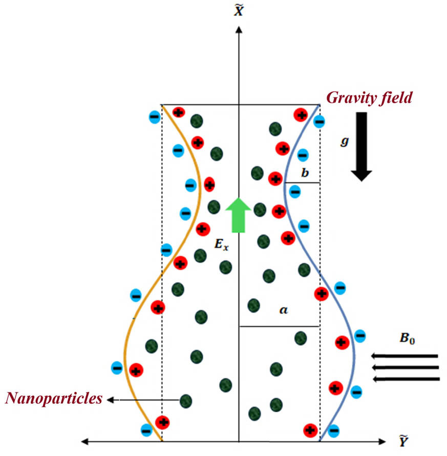
The lower channel wall’s temperature as well as the concentration fields are maintained at T o and C o , while the upper channel walls are maintained at T 1 and C 1 .

Figure 1

A diagram of EOF accompanied by peristalsis.

Microchannel geometry can be represented mathematically as [47]

(1) Y ∼ = h ∼ ( X ∼ , t ∼ ) = a + b sin 2 π ( X ∼ − c t ∼ ) λ .

2.2 Governing equations

The EOF of a micropolar nanofluid in an electromagnetohydrodynamic (EMHD) environment is controlled by the following formulas in the laboratory frame [37,47,48,49]:

Continuity equation:

(2) ∂ U ∼ ∂ X ∼ + ∂ V ∼ ∂ Y ∼ = 0 .

Equation of motion:

(3) ρ f ∂ U ∼ ∂ t ∼ + U ∼ ∂ U ∼ ∂ X ∼ + V ∼ ∂ U ∼ ∂ Y ∼ = − ∂ P ∼ ∂ X ∼ + ( μ + k ) ∂ 2 U ∼ ∂ X ∼ 2 + ∂ 2 U ∼ ∂ Y ∼ 2 + k ∂ ω ∼ ∂ Y ∼ + σ ( E 0 B 0 − B 0 2 U ∼ ) − ( μ + k ) k 0 U ∼ + ( 1 − C O ) ρ f β g ( T ∼ − T 0 ) − ( ρ p − ρ f ) g ( C ∼ − C 0 ) − ( N ∼ − N 0 ) g γ ( ρ m − ρ p ) + ρ e E x ,

(4) ρ f ∂ V ∼ ∂ t ∼ + U ∼ ∂ V ∼ ∂ X ∼ + V ∼ ∂ V ∼ ∂ Y ∼ = − ∂ P ∼ ∂ Y ∼ + ( μ + k ) ∂ 2 V ∼ ∂ X ∼ 2 + ∂ 2 V ∼ ∂ Y ∼ 2 − k ∂ ω ∼ ∂ X ∼ − ( μ + k ) k 0 V ∼ + ( 1 − C O ) ρ f β g ( T ∼ − T 0 ) − ( ρ p − ρ f ) g ( C ∼ − C 0 ) − ( N ∼ − N 0 ) g γ ( ρ m − ρ p ) .

Equation of microrotation motion:

(5) ρ f J ∼ ∂ ω ∼ ∂ t ∼ + U ∼ ∂ ω ∼ ∂ X ∼ + V ∼ ∂ ω ∼ ∂ Y ∼ = − 2 k ω ∼ + γ * ∂ 2 ω ∼ ∂ X ∼ 2 + ∂ 2 ω ∼ ∂ Y ∼ 2 + k ∂ V ∼ ∂ X ∼ − ∂ U ∼ ∂ Y ∼ .

Energy equation with viscous dissipation:

(6) ∂ T ∼ ∂ t ∼ + U ∼ ∂ T ∼ ∂ X ∼ + V ∼ ∂ T ∼ ∂ Y ∼ = α 1 ∂ 2 T ∼ ∂ X ∼ 2 + ∂ 2 T ∼ ∂ Y ∼ 2 = ( ρ c p ) p ( ρ c p ) f D B ∂ C ∼ ∂ X ∼ ∂ T ∼ ∂ X ∼ + ∂ C ∼ ∂ Y ∼ ∂ T ∼ ∂ Y ∼ + D T T 0 ∂ T ∼ ∂ X ∼ 2 + ∂ T ∼ ∂ Y ∼ 2 + σ ( ρ c p ) f ( U ∼ B 0 − E 0 ) 2 + D m k T C s ( ρ c p ) f ∂ 2 C ∼ ∂ X ∼ 2 + ∂ 2 C ∼ ∂ Y ∼ 2 + ( μ + k ) ( ρ c p ) f 4 ∂ U ∼ ∂ X ∼ 2 + ∂ V ∼ ∂ X ∼ + ∂ U ∼ ∂ Y ∼ 2 .

Concentration equation:

(7) ∂ C ∼ ∂ t ∼ + U ∼ ∂ C ∼ ∂ X ∼ + V ∼ ∂ C ∼ ∂ Y ∼ = D B ∂ 2 C ∼ ∂ X ∼ 2 + ∂ 2 C ∼ ∂ Y ∼ 2 + D T T 0 ∂ 2 T ∼ ∂ X ∼ 2 + ∂ 2 T ∼ ∂ Y ∼ 2 + D B k T T m ∂ 2 T ∼ ∂ X ∼ 2 + ∂ 2 T ∼ ∂ Y ∼ 2 − k 1 ( C ∼ − C 0 ) .

Microorganisms’ equation:

(8) ∂ N ∼ ∂ t ∼ + U ∼ ∂ N ∼ ∂ X ∼ + V ∼ ∂ N ∼ ∂ Y ∼ = D m ∂ 2 N ∼ ∂ Y ∼ 2 − bW c ( C 1 − C 0 ) N ∼ ∂ 2 C ∼ ∂ Y ∼ 2 + ∂ N ∼ ∂ Y ∼ ∂ C ∼ ∂ Y ∼ ,

where U ∼ , V ∼ , ω ∼ , T ∼ , C ∼ , N ∼ , J ∼ , P , μ , k , and γ * constitute the speeds in the directions of X ∼ and Y ∼ , microrotation vector, temperature profile, concentration profile, microorganism profile, micro-gyration parameter, fluid pressure, and viscosity constants for dynamic and micropolar fluids, in each case. Also, here, ρ f signifies the density of the nanofluid, σ f is the nanofluid’s conductivity of electricity, ρ e is the overall density of charges, E x is the acceleration in the x-orientation of the electrical field, B 0 signifies the field of magnetized attraction, β is the volume expansion factor, and k 0 is the permeability constant of the permeable substance. α 1 = k * ( ρ c p ) f . where k * is the diffusivity of thermal expansion, ( ρ c p ) p signifies the effective heat capacitance of nanomaterials, C ∼ indicates the dispersion of the nanomaterial’s concentration, D T denotes the thermophoretic diffusion coefficient, and D B is the Brownian diffusion. D and K T symbolize the corresponding mass diffusivity and the ratio of thermal diffusion. N ∼ is the percentage of mobile bacteria in the microorganism’s whole size, b is the chemotaxis constant, and W c is the fastest pace at which a cell can swim. ρ p , ρ m , and γ are the nanoparticle density, the density of microorganisms, and the typical number of microbes, respectively. It is assumed that bW _c is a constant product, and k 1 stands for chemical reaction rate.

2.2.1 EHD [47]

In a microscopic channel, Poisson’s equation [25] is defined as follows:

(9) ∇ 2 Φ ∼ = − ρ e ε ,

where Φ ∼ , ε , and ρ e stand for the potential of electricity, dielectric permeability, and the overall charge density, respectively.

2.2.2 Potential distributions

Consistent with the distributions of Boltzmann [50], the total density of charges ρ e is as follows:

(10) ρ e = − Z ν e ( n ∼ − − n ∼ + ) .

The definition of the anions ( n ∼ − ) and cations ( n ∼ + ) in this situation are

(11) n ∼ − = n ∼ 0 exp − e Z ν T a ν K B Φ ∼ , n ∼ + = n ∼ 0 exp + e Z ν T a ν K B Φ ∼ ,

where n ∼ 0 symbolizes the concentration, Z ν is the balance of charges, K B is the Boltzmann’s constant, e is the electrical charge, and T av is the typical temperature. The principle of Debye–Hückel is a linearization state e Z ν T a ν K B ≪ 1 . Eq. (10) is lowered to

(12) ρ e = − ϵ λ D 2 Φ ∼ .

Given that Eq. (9) yields

(13) d 2 Φ ∼ d y ∼ 2 = 1 λ D 2 Φ ∼ ,

where λ D = ( e Z ν ) − 1 ϵ T a ν K B 2 n 0 . Using the dimensionless quantities that follow

(14) Φ = Φ ∼ ζ , Y = y ∼ a .

Eq. (13) therefore becomes

(15) d 2 Φ d y 2 = m e 2 Φ ,

where m e = a λ D represents the parameter for electroosmosis. With the boundary constraints ∂ Φ ∂ y = 0 at y = 0 and Φ = 1 at y = h , the mathematical solution of Eq. (15) is as follows [47]:

(16) Φ = cosh m e y cosh m e h .

2.2.3 Boundary under certain conditions, the lubrication technique, and non-dimensionalities

The fluctuating boundary causes the motion to be erratic within the stationary frame ( X ∼ , Y ∼ ) . Nevertheless, caused by the static border, it can be regarded as steady when evaluated in a movable frame ( x ∼ , y ∼ ) . Consequently, Noreen [51] represents the translational transition between the following frames:

(17) x ∼ = X ∼ − c t ∼ , y ∼ = Y ∼ , u ∼ ( x ∼ , y ∼ ) = U ∼ ( X ∼ , Y ∼ , t ∼ ) − c , v ∼ ( x ∼ , y ∼ ) = V ∼ ( X ∼ , Y ∼ , t ∼ ) , P ∼ ( x ∼ , y ∼ ) = P ∼ ( X ∼ , Y ∼ , t ∼ ) , T ∼ ( x ∼ , y ∼ ) = T ∼ ( X ∼ , Y ∼ , t ∼ ) , C ∼ ( x ∼ , y ∼ ) = C ∼ ( X ∼ , Y ∼ , t ∼ ) , N ∼ ( x ∼ , y ∼ ) = N ∼ ( X ∼ , Y ∼ , t ∼ ) , ω ∼ ( x ∼ , y ∼ ) = ω ∼ ( X ∼ , Y ∼ , t ∼ ) .

Applying the changes described in (17), the continuation, momentum, microrotation, energy, quantity, and microorganisms within the waveform frame referencing Eqs. (2)–(8) can be expressed as [41,49,52,53,54] follows.

Continuity equation:

(18) ∂ u ∼ ∂ x ∼ + ∂ v ∼ ∂ y ∼ = 0 .

Equation of motion:

(19) ρ u ∼ ∂ u ∼ ∂ x ∼ + v ∼ ∂ u ∼ ∂ y ∼ = − ∂ p ∼ ∂ x ∼ + ( μ + k ) ∂ 2 u ∼ ∂ x ∼ 2 + ∂ 2 u ∼ ∂ y ∼ 2 + k ∂ ω ∼ ∂ y ∼ + ( 1 − C O ) ρ f β g ( T ∼ − T 0 ) − ( ρ p − ρ f ) g ( C ∼ − C 0 ) − ( N ∼ − N 0 ) g γ ( ρ m − ρ p ) + σ ( E 0 B 0 − B 0 2 ( u ∼ + c ) ) − ( μ + k ) k 0 ( u ∼ + c ) + ρ e E x ,

(20) ρ u ∼ ∂ v ∼ ∂ x ∼ + v ∼ ∂ v ∼ ∂ y ∼ = − ∂ p ∼ ∂ y ∼ + ( μ + k ) ∂ 2 v ∼ ∂ x ∼ 2 + ∂ 2 v ∼ ∂ y ∼ 2 − k ∂ ω ∼ ∂ x ∼ + ( 1 − C O ) ρ f β g ( T ∼ − T 0 ) − ( ρ p − ρ f ) g ( C ∼ − C 0 ) − ( N ∼ − N 0 ) g γ ( ρ m − ρ p ) − μ k 0 v ∼ .

Equation of microrotation motion:

(21) ρ J ∼ u ∼ ∂ ω ∼ ∂ x ∼ + v ∼ ∂ ω ∼ ∂ y ∼ = − 2 k ω ∼ + γ * ∂ 2 ω ∼ ∂ x ∼ 2 + ∂ 2 ω ∼ ∂ y ∼ 2 + k ∂ v ∼ ∂ x ∼ − ∂ u ∼ ∂ y ∼ .

Energy equation with viscous dissipation:

(22) u ∼ ∂ T ∼ ∂ x ∼ + v ∼ ∂ T ∼ ∂ y ∼ = α 1 ∂ 2 T ∼ ∂ x ∼ 2 + ∂ 2 T ∼ ∂ y ∼ 2 + τ D B ∂ C ∼ ∂ x ∼ ∂ T ∼ ∂ x ∼ + ∂ C ∼ ∂ y ∼ ∂ T ∼ ∂ y ∼ + D T T 0 ∂ T ∼ ∂ x ∼ 2 + ∂ T ∼ ∂ y ∼ 2 + σ ( ρ c ) f ( ( u ∼ + c ) B 0 − E 0 ) 2 + D m k T C s ( Cp ) f ∂ 2 C ∼ ∂ x ∼ 2 + ∂ 2 C ∼ ∂ y ∼ 2 + ( μ + k ) ( ρ c p ) f 4 ∂ u ∼ ∂ x ∼ 2 + ∂ v ∼ ∂ x ∼ + ∂ u ∼ ∂ y ∼ 2 .

Concentration equation:

(23) u ∼ ∂ C ∼ ∂ x ∼ + v ∼ ∂ C ∼ ∂ y ∼ = D B ∂ 2 C ∼ ∂ x ∼ 2 + ∂ 2 C ∼ ∂ y ∼ 2 + D T T 0 ∂ 2 T ∼ ∂ x ∼ 2 + ∂ 2 T ∼ ∂ y ∼ 2 + D B k T T m ∂ 2 T ∼ ∂ x ∼ 2 + ∂ 2 T ∼ ∂ y ∼ 2 − k 1 ( C ∼ − C 0 ) .

Microorganisms’ equation:

(24) u ∼ ∂ N ∼ ∂ x ∼ + V ∼ ∂ N ∼ ∂ x ∼ = D m ∂ 2 N ∼ ∂ y ∼ 2 − bW c ( C 1 − C 0 ) N ∼ ∂ 2 C ∼ ∂ y 2 + ∂ N ∼ ∂ y ∼ ∂ C ∼ ∂ y ∼ .

Familiarizing the nondimensional variables:

(25) x = 2 π λ x ∼ , y = y ∼ a , u = u ∼ c , v = v ∼ c , p = 2 π a 2 λ c μ p ∼ , δ = 2 π a λ , Φ = Φ ∼ a , h = h ∼ a , Φ = Φ ∼ ζ , θ = T ∼ − T 0 T 1 − T 0 , φ = C ∼ − C 0 C 1 − C 0 , ξ = N ∼ − N 0 N 1 − N 0 , ω = a ω ∼ c , J = J ∼ a 2 , R e = ρ f ca μ , G r = ρ f g β a 2 ( 1 − C 0 ) ( T 1 − T 0 ) μ c , N r = ( ρ p − ρ f ) ( C 1 − C 0 ) ( 1 − C O ) β ρ f ( T 1 − T 0 ) , R b = γ ( ρ m − ρ p ) ( N 1 − N 0 ) ( 1 − C O ) β ρ f ( T 1 − T 0 ) , M = σ μ a B o , E 1 = E o c B 0 , D a = k o a 2 , m e = a λ D , U HS = − ζ ϵ E x c μ , N = k ( μ + k ) , m 2 = a 2 k ( 2 μ + k ) γ * ( μ + k ) , α = k * ( ρ c p ) f , S c = ν f D B , S r = ρ f D B k T T m μ ( T 1 − T 0 ) ( C 1 − C 0 ) , γ 1 = k 1 a 2 ν f , L b = ν f D m , P e = b W c D m , Ω = N 0 N 1 − N 0 , E c = c 2 ( c p ) f ( T 1 − T o ) , D u = D B k T c s ( c p ) f μ ( C 1 − C 0 ) ( T 1 − T 0 ) , P r = μ α ρ f , N t = ( ρ c p ) p ρ f D T ( T 1 − T 0 ) ( ρ c p ) f μ T 0 , N b = ( ρ c p ) p ρ f D B ( C 1 − C 0 ) ( ρ c p ) f μ .

Here, φ , ξ , ω , J , R e , G r , N r , R b , M , E 1 , D a , m e , U HS , N , m 2 , S c , S r , γ 1 , L b , P e , Ω , E c , D u , P r , N b , and N t represent the non-dimensional temperature’s function, amount of nanoparticles, motile microorganism profile density, microrotation function, non-dimensional micro-gyration parameter, Reynolds number, the local temperature’s Grashof number and the buoyancy proportion, bioconvection Rayleigh number, magnetic field, electric field, Darcy number, electroosmotic parameter, Helmholtz–Smoluchowski velocity, coupling number, micropolar parameter, the Schmidt, Soret numbers, chemically reactive variable, Lewis number for bioconvection and Peclet coefficient, the ratio of motile microorganism, Eckert number, Dufour number, Prandtl number, the Brownian motion and characteristics of thermophoresis, respectively. After removing the bars, we obtain [41,49,52,53,54] by applying the non-dimensional variables (25), which are the controlling flow field equations (Eqs. (18)–(24)).

Continuity equation:

(26) δ ∂ u ∂ x + ∂ v ∂ y = 0 ,

Equation of motion:

(27) R e δ u ∂ u ∂ x + v ∂ u ∂ y = − ∂ p ∂ x + 1 1 − N N ∂ ω ∂ y + δ ∂ 2 u ∂ x 2 + ∂ 2 u ∂ y 2 + G r ( θ − N r φ − R b ξ ) + M 2 ( E 1 − ( u + 1 ) ) − 1 ( 1 − N ) D a ( u + 1 ) + U HS m e 2 Φ ,

(28) R e δ δ u ∂ v ∂ x + v ∂ v ∂ y = − ∂ p ∂ y + 1 1 − N δ 3 ∂ 2 v ∂ x 2 − δ 2 N ∂ ω ∂ x + δ ∂ 2 v ∂ y 2 + δ G r ( θ − N r φ − R b ξ ) − 1 ( 1 − N ) D a δ v .

Equation of microrotation motion:

(29) R e J 1 − N N δ u ∂ ω ∂ x + v ∂ ω ∂ y = − 2 ω + 2 − N m 2 δ 2 ∂ 2 ω ∂ x 2 + ∂ 2 ω ∂ y 2 + δ ∂ v ∂ x − ∂ u ∂ y .

Energy equation with viscous dissipation:

(30) R e δ u ∂ θ ∂ x + v ∂ θ ∂ y = 1 P r δ 2 ∂ 2 θ ∂ x 2 + ∂ 2 θ ∂ y 2 + N b δ 2 ∂ φ ∂ x ∂ θ ∂ x + ∂ φ ∂ y ∂ θ ∂ y + N t δ 2 ∂ θ ∂ x 2 + ∂ θ ∂ y 2 + M 2 E c ( ( u + 1 ) − E 1 ) 2 + D u δ 2 ∂ 2 φ ∂ x 2 + ∂ 2 φ ∂ y 2 + 1 1 − N E c 4 δ ∂ u ∂ x 2 + δ ∂ v ∂ x + ∂ u ∂ y 2 .

Concentration equation:

(31) R e δ u ∂ φ ∂ x + v ∂ φ ∂ y = 1 S c δ 2 ∂ 2 φ ∂ x 2 + ∂ 2 φ ∂ y 2 + S r δ 2 ∂ 2 θ ∂ x 2 + ∂ 2 θ ∂ y 2 + N t N b 1 S c δ 2 ∂ 2 θ ∂ x 2 + ∂ 2 θ ∂ y 2 − γ 1 φ .

Microorganism equation:

(32) L b R e δ u ∂ ξ ∂ x + v ∂ ξ ∂ y = ∂ 2 ξ ∂ y 2 − P e ( ξ + Ω ) ∂ 2 φ ∂ y 2 + ∂ ξ ∂ y ∂ φ ∂ y .

In the context of the stream characteristic ψ , the nondimensional components of velocity ( u , v ) are connected through the subsequent relationships:

(33) u = ∂ ψ ∂ y , v = − δ ∂ ψ ∂ x .

Eq. (26) is met in the same way once Eq. (33) is introduced, and Eqs. (27)–(32) are as follows [37,47,49,52,53].

Equation of motion :

(34) R e δ ∂ ψ ∂ y ∂ 2 ψ ∂ x ∂ y − ∂ ψ ∂ x ∂ 2 ψ ∂ y 2 = − ∂ p ∂ x + 1 1 − N N ∂ ω ∂ y + δ 2 ∂ 2 ∂ x 2 ∂ ψ ∂ y + ∂ 2 ∂ y 2 ∂ ψ ∂ y + G r ( θ − N r φ − R b ξ ) + M 2 E 1 − ∂ ψ ∂ y + 1 − 1 ( 1 − N ) D a ∂ ψ ∂ y + 1 + U HS m e 2 Φ ,

(35) − R e δ 3 ∂ ψ ∂ y ∂ 2 ψ ∂ x 2 − ∂ ψ ∂ x ∂ 2 ψ ∂ x ∂ y = − ∂ p ∂ y + 1 1 − N δ 3 ∂ 2 ∂ x 2 − δ ∂ ψ ∂ x − δ 2 N ∂ ω ∂ x + δ ∂ 2 ∂ y 2 − δ ∂ ψ ∂ x + δ G r ( θ − N r φ − R b ξ ) + 1 ( 1 − N ) D a δ 2 ∂ ψ ∂ x .

Equation of microrotation motion:

(36) R e J 1 − N N δ ∂ ψ ∂ y ∂ ω ∂ x − δ ∂ ψ ∂ x ∂ ω ∂ y = − 2 ω + 2 − N m 2 δ 2 ∂ 2 ω ∂ x 2 + ∂ 2 ω ∂ y 2 + − δ 2 ∂ 2 ψ ∂ x 2 − ∂ 2 ψ ∂ y 2 .

Energy equation with viscous dissipation:

(37) R e δ ∂ ψ ∂ y ∂ θ ∂ x − δ ∂ ψ ∂ x ∂ θ ∂ y = 1 P r δ 2 ∂ 2 θ ∂ x 2 + ∂ 2 θ ∂ y 2 + N b δ 2 ∂ φ ∂ x ∂ θ ∂ x + ∂ φ ∂ y ∂ θ ∂ y + N t δ 2 ∂ θ ∂ x 2 + ∂ θ ∂ y 2 + M 2 E c ∂ ψ ∂ y + 1 − E 1 2 + δ 2 ∂ 2 φ ∂ x 2 + ∂ 2 φ ∂ y 2 + 1 1 − N E c 4 δ ∂ ∂ x ∂ ψ ∂ y 2 + δ ∂ ∂ x − δ ∂ ψ ∂ x + ∂ ∂ y ∂ ψ ∂ y 2 .

Concentration equation:

(38) R e δ ∂ ψ ∂ y ∂ φ ∂ x − δ ∂ ψ ∂ x ∂ φ ∂ y = 1 S c δ 2 ∂ 2 φ ∂ x 2 + ∂ 2 φ ∂ y 2 + S r δ 2 ∂ 2 θ ∂ x 2 + ∂ 2 θ ∂ y 2 + N t N b 1 S c δ 2 ∂ 2 θ ∂ x 2 + ∂ 2 θ ∂ y 2 − γ 1 φ .

Microorganism equation:

(39) L b R e δ ∂ ψ ∂ y ∂ ξ ∂ x − δ ∂ ψ ∂ x ∂ ξ ∂ y = ∂ 2 ξ ∂ y 2 − P e ( ξ + Ω ) ∂ 2 φ ∂ y 2 + ∂ ξ ∂ y ∂ φ ∂ y .

Considering the extended wavelengths δ ≥ 1 along with the small Reynolds numbers, we obtain the subsequent equations without considering the concepts of degree δ and higher order:

(40) ∂ p ∂ x = 1 1 − N N ∂ ω ∂ y + ∂ 2 ∂ y 2 ∂ ψ ∂ y + G r ( θ − N r φ − R b ξ ) + M 2 E 1 − ∂ ψ ∂ y + 1 ︸ EMHD forces − 1 ( 1 − N ) D a ∂ ψ ∂ y + 1 ︸ Darcian te r m + U HS m e 2 ︸ Φ electroosmotic forces ︸ EOF ,

(41) ∂ p ∂ y = 0 ,

(42) 1 P r ∂ 2 θ ∂ y 2 + N b ∂ φ ∂ y ∂ θ ∂ y + N t ∂ θ ∂ y 2 + M 2 E c ∂ ψ ∂ y + 1 − E 1 ︸ Joule Heating 2 + D u ∂ 2 φ ∂ y 2 + 1 1 − N E c ∂ 2 ψ ∂ y 2 2 ︸ Viscous Dissipation = 0 ,

(43) − 2 ω + 2 − N m 2 ∂ 2 ω ∂ y 2 − ∂ 2 ψ ∂ y 2 = 0 ,

(44) ∂ 2 φ ∂ y 2 + S r S c ∂ 2 θ ∂ y 2 + N t N b ∂ 2 θ ∂ y 2 − γ 1 φ S c = 0 ,

(45) ∂ 2 ξ ∂ y 2 − P e ( ξ + Ω ) ∂ 2 φ ∂ y 2 + ∂ ξ ∂ y ∂ φ ∂ y = 0 .

When pressure is removed from Eq. (40) as well as Eq. (41), we obtain

(46) 1 1 − N ∂ ∂ y N ∂ ω ∂ y + ∂ 3 ψ ∂ y 3 + G r ∂ θ ∂ y − N r ∂ φ ∂ y − R b ∂ ξ ∂ y − M 2 ∂ 2 ψ ∂ y 2 ︸ EMHD forces − 1 ( 1 − N ) D a ∂ 2 ψ ∂ y 2 ︸ Darcian te r m + U HS m e 2 ︸ ∂ Φ ∂ y electroosmotic forces ︸ EOF = 0 .

Under conditions [55]:

(47) ∂ 2 ψ ∂ y 2 = 0 , ψ = 0 , ∂ θ ∂ y = 0 , ∂ φ ∂ y = 0 , ∂ ω ∂ y = 0 , ∂ ξ ∂ y = 0 at y = 0 , ∂ ψ ∂ y + γ 3 ∂ 2 ψ ∂ y 2 = − 1 , ψ = f , θ + γ 2 ∂ θ ∂ y = 0 , φ + γ 4 ∂ φ ∂ y = 0 , ω + γ 5 ∂ ω ∂ y = 0 , ξ + γ 6 ∂ ξ ∂ y = 0 at y = h = 1 + ε 1 sin x .

The boundary conditions applied in this study reflect realistic physical constraints commonly encountered in microfluidic environments. At the lower wall, no-slip and insulation conditions are assumed, implying that there is no penetration of fluid, heat, mass, microrotation, or microorganisms across the wall. This represents a thermal and mass-insulated surface with no microrotational effects. At the upper peristaltically oscillating wall, velocity, thermal, concentration, microrotation, and microorganism slip conditions are incorporated to account for the partial interaction between the wall and fluid. These slip conditions simulate more accurate physical behaviors, where the wall may allow limited transfer or interaction due to surface characteristics or biological coatings. Collectively, these boundary settings allow the model to realistically capture the influences of wall dynamics and surface attributes on electroosmotic peristalsis flow of micropolar bio-nanofluids. Here, f is the average circulation rate of the moving frame’s devoid of dimensions, and Θ is the average rate of flow without dimensions in each frame. Moreover, the relationship between f within the movable frame and Θ within the stationary structure is as follows [41,47,52,53,54]:

(48) Θ = f + 1 ,

where f = ∫ 0 h ( x ) ∂ ψ ∂ y d y = ψ ( h ( x ) − ψ ( 0 ) ) .

The following are the non-dimensional formulas [41,52,53,54] describing the rate of pressure surge for wavelength ∆ P :

(49) ∆ P = ∫ 0 1 d P d x d x .

3 Computational methodology

The use of mathematical models to address real-world issues has become crucial in several aspects of contemporary life for elucidating, delineating, or forecasting a wide array of phenomena. To exemplify these challenges, scientists often use a set of very intricate non-linear linked equations derived from partial differential equations. Analytical solutions for such challenges are often unattainable. We can efficiently and dependably manage this degree of complexity due to our expertise in numerous prominent computational programming languages. Mathematica, an advanced and completely integrated software programming language, has been used in our problem-solving endeavors. A systematic and successful methodology for addressing the complexity of solving the governing system of equations has been established with the built-in command, parametric estimate NDSolve. This numerical approach provides substantial benefits by decreasing mistakes and reducing CPU time per evaluation. This built-in tool generates a suitable method for numerical computations and produces the corresponding graphical output. According to the selected convergence criterion, the difference between consecutive solution values must be less than 10⁻⁶ to guarantee good precision.

4 Verification of the outcomes

To demonstrate the validity of our current work, we compare our numerical approach for dimensionless velocity and the results of two earlier studies [54,41], concentrating on a particular case. Many phenomena are disregarded in this comparison, including the mass and heat transmission of the liquid, the motion of organisms in the non-existence of the porous material in the channel, and, most importantly, the impact of the field of magnetic attraction. Table 2 contrasts the speed profiles of the two scenarios – the hydrodynamic case [54] and the EHD instance [41] – to show how our model compares with the findings given by Ali and Hayat [54] and Noreen et al. [41]. To enable pertinent comparisons, we have set G r = 0 , G c = 0 , M = 0 , γ 2 = γ 3 = γ 4 = 0 , U HS = 0 , m e = 0.001 , and D a → ∞ . As a result, the results we obtained from the methodology are in good agreement with these analytical techniques.

Table 2

Velocity profile u ( x , y ) comparison for various coupling numbers N and micropolar parameter m values when G r = 0 , G c = 0 , M = 0 , γ 2 = γ 3 = γ 4 = 0 , and D a → ∞

Microrotation m	Coupling number N	Hydrodynamic case [54] ( U HS = 0 , m e = 0.001 )	Current study	EHD Case. [41] ( U HS = 0.5 , m e = 6 )	Current study
1	0.2	−1	−1	2.49730	2.45870
10	0.2	−1	−1	3.00531	3.01260
100	0.2	−1	−1	3.28171	3.27924
100	0.3	6.173850	6.17425	3.25985	3.25478
100	0.4	6.739920	6.73578	3.23800	3.23576
100	0.5	7.111769	7.11234	3.21614	3.21458

5 Computational discussion of the results

The physical structure of the problem comprises a microchannel, which is a simplified but accurate depiction of microfluidic devices encountered in real-world applications. In the above structure, the addition of an electric field from the outside E x promotes the formation of electroosmotic forces. These forces are influenced by the unique characteristics of micropolarity liquids, such as interior microrotational movement. Furthermore, the thickness and distribution of charges of the EDL may have an impact on the size and direction of the EOF. The double layer’s thickness additionally affects the EOF; thicker layers of double thickness have lower flow rates. On a physical level, the electric body force fluctuates precisely according to E x , demonstrating that a thicker EDL causes a significant drop in the electrical body force. The wavelength typically varies between a few millimeters and 100 μm. Some have been identified as constants, such as e (the electron charge) and K _B (the constant of Boltzmann). Generally, the wave speed ranges between 1 and 10 mm/s⁻¹. The wave’s amplitude, which typically ranges between 10 and 200 μm, represents the largest divergence from the standard deviation position. The conduit width d for peristaltic flow typically spans from 1 to 10 mm. The material constants are k , μ , and γ * . These parameter ranges vary according to the experimental conditions, microscopic structure, and rotational kinematics. This section addresses the effects of diverse configurations (i.e., slippage temperature 0.02 ≤ γ 2 ≤ 0.05 , electroosmotic parameter 0.0 ≤ m e ≤ 6.0 , maximal electroosmotic velocity, and Helmholtz–Smoluchowski speed − 0.2 ≤ U HS ≤ 0.1 , Peclet number 0.5 ≤ P e ≤ 0.8 , the bioconvection constant 0.5 ≤ Ω ≤ 0.8 , thermophoresis parameter 0.01 ≤ N t ≤ 0.04 , Brownian motion parameter 0.5 ≤ N b ≤ 0.8 , coupling number 0.0 ≤ N ≤ 0.6 , Darcy number 0.1 ≤ D a ≤ 0.4 , and magnetic field parameter 1.0 ≤ M ≤ 1.3 ) on the velocity distribution u ( x , y ) , temperature distribution θ ( x , y ) , concentration distribution ϕ ( x , y ) , motile microorganism distribution ξ ( x , y ) , concentration distribution ω ( x , y ) , stream lines patterns ψ ( x , y ) , and heat transfer rate Z [41,47]. Figures 2–8 are included for this reason. To capture spatial variations along the channel, results are evaluated at two distinct axial positions: x = π 2 , x = 3 π 2 , representing different cross-sections within one wavelength of the peristaltic wave. This allows for a comparative understanding of flow characteristics at various locations along the channel.

$Figure 2 Velocity distribution for (a) N N , (b) D a {D}_{a} , (c) m e {m}_{e} , and (d) U HS {U}_{{\rm{HS}}} .$

Figure 2

Velocity distribution for (a) N , (b) D a , (c) m e , and (d) U HS .

$Figure 3 Temperature distribution for (a) γ 2 {\gamma }_{2} , (b) M M , (c) m e {m}_{e} , and (d) U HS {U}_{{\rm{HS}}} .$

Figure 3

Temperature distribution for (a) γ 2 , (b) M , (c) m e , and (d) U HS .

$Figure 4 Motile density of microorganism’s distribution for (a) N b {N}_{b} , (b) N t {N}_{t} , (c) P e {P}_{e} , and (d) Ω \Omega .$

Figure 4

Motile density of microorganism’s distribution for (a) N b , (b) N t , (c) P e , and (d) Ω .

$Figure 5 Concentration distribution for (a) γ 4 {\gamma }_{4} , (b) M M , (c) m e {m}_{e} , and (d) U HS {U}_{{\rm{HS}}} .$

Figure 5

Concentration distribution for (a) γ 4 , (b) M , (c) m e , and (d) U HS .

$Figure 6 Microrotation velocity distribution for (a) γ 5 {\gamma }_{5} , (b) N N , (c) M M , and (d) E 1 {E}_{1} .$

Figure 6

Microrotation velocity distribution for (a) γ 5 , (b) N , (c) M , and (d) E 1 .

$Figure 7 The rate of heat transmission for (a) M M , (b) E c {E}_{c} , (c) m e {m}_{e} , and (d) N t {N}_{t} .$

Figure 7

The rate of heat transmission for (a) M , (b) E c , (c) m e , and (d) N t .

$Figure 8 Distribution of microrotation velocity for (a) U HS {U}_{{\rm{HS}}} , (b) M M , (c) m m , and (d) m e {m}_{e} .$

Figure 8

Distribution of microrotation velocity for (a) U HS , (b) M , (c) m , and (d) m e .

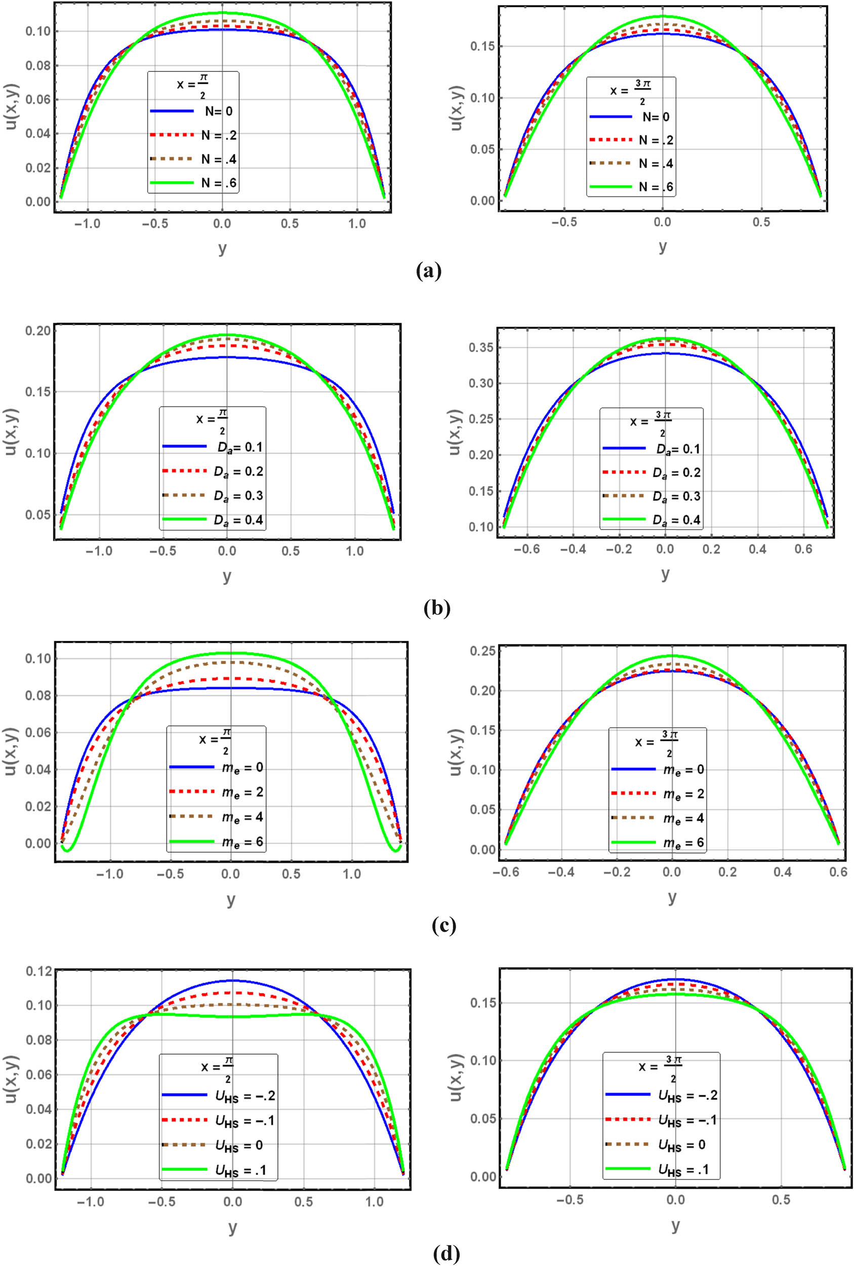
5.1 Velocity profile

This section discusses the implications of the coupling number N , Darcy number D a , the electroosmotic factor m e , the maximal electroosmotic velocity, and Helmholtz–Smoluchowski velocity U HS on the distributions of velocity, which, in turn, are shown in Figure 2(a–d). First, we investigated the influence of diverse variables upon the speed profile and compared them at different sectors of the channel. We found that the influence of speed when changing these variables improves significantly at x = π 2 than at x = 3 π 2 . The data indicate that the velocity charts have a descending concavity. These graphs illustrate a parabolic trajectory, with the apex situated in the center of the channel. The impact of the coupling number N on the axial speed is shown in Figure 2(a). The micropolar parameter explains spin diffusion. It is possible to reduce the micropolar liquid description to the Newtonian liquid theory for k → ∞ . It is seen that the circulation reversing trend occurred around the conduit’s walls, but it increases towards the channel’s middle line as the coupling number increases. Figure 2(b) illustrates how the fluid speed is influenced by the Darcy numbers. The velocity of the axial direction decreases as one gets close to the channel walls and increases as the Darcy number increases toward the channel center. Under similar conditions, the parameter for electroosmotic characterizes the EDL’s thickness (that is, for m e → ∞ , EDL is extremely thin; it can be emotionally deduced that liquid flowing is unaffected by the arrangement of electrons throughout the wall’s surface), and Helmholtz–Smoluchowski velocity symbolizes the consequence of an electric field that is applied externally. If U HS → 0 , the issue will arise from the peristalsis transference of micropolar liquid through a symmetric channel. According to Figure 2(c), m e raises the magnitude of u ( x , y ) , indicating that u ( x , y ) increases as m e increases in the channel’s center and reduces as it approaches the channel’s walls, as m e equals the channel height divided by Debye’s length λ D . This implies that λ D and EDL are inversely proportional. As a result, the middle region, y = 0 , has a greater fluid flow. Zeta potential is a commonly used representation of the electroosmotic parameter. It is an indication of the outermost density of charge at the fluid–solid contact. The zeta potential controls the EOF’s amplitude, direction, and velocity. In essence, the electroosmotic variable gauges a liquid’s ability to move across a charged surface when an electrical field exists. Again, the flow is a simple hydrodynamic for m e → 0 , and EHD at a particular m e value. The hydrodynamic flow curve is positioned beneath the EHD flow outlines, indicating that the velocity profile is influenced by the applied electric field. Figure 2(d) depicts that u ( x , y ) decreases as U HS increases in y = 0 ; conversely, an opposing movement is observed at y = h ( x ) . According to the physical conclusion U HS , fluid velocity drops, as the EDL thickness increases. As a result, when EDL is present, fluid flow reduces. Physically, the Helmholtz–Smoluchowski velocity is a physical representation of the equilibrium between the frictional forces of the fluid and the force of electricity operating on the charged particle. Specifically, the mean particle velocity, excluding the impact of extraneous external factors like viscoelastic drag or gravity, is known as the Helmholtz–Smoluchowski velocity. For purely hydrodynamic flow, the velocity is shown by the curve for U HS → 0 .

5.2 Temperature profile

Figure 3(a–d) depicts the temperature change with pertinent fluid parameters. Temperature profiles, like velocity profiles, display the graph’s parabolic form, with the highest possible temperature occurring in the center. The change in the temperature slip parameter γ 2 , or an increasing amount of γ 2 , on the operating temperature outlines are described, as shown in Figure 3(a). It is clear from the provided findings that the temperature outline increases. Figure 3(b) demonstrates how the ambient temperature distribution is influenced by the field’s magnetic parameter M. It is obvious from the figure that the environmental temperature outline increases when the magnetized force impact is larger than its tendency to reverse the flow. Also, Figure 3(c) displays that θ ( x , y ) increases with increasing m e . Hence, the reduction in EDL increases θ ( x , y ) significantly. Figure 3(d) shows the consequences of extreme electroosmotic velocity U HS on θ ( x , y ) . It indicates that for more values of U HS , θ ( x , y ) declines. Furthermore, Figure 3(c) shows that when m e increases, θ ( x , y ) also increases. As a result, there is a notable increase in θ ( x , y ) when EDL decreases. The impact of maximal electroosmotic acceleration U HS on θ ( x , y ) is shown in Figure 3(d), and indicates that θ ( x , y ) decreases when U HS values increase.

5.3 Density of motile microorganism profiles

Figure 4(a–d) shows the activities of motile microorganism profiles for various values of physical factors. It can be established from Figure 4(a) that as the Brownian diffusion variable N b increases the density of the motile microbe profile also increases. It is obvious that an increase in N b results in a higher transfer rate of motile microorganisms. The effect of the parameter used for thermophoresis N t on the motile microorganisms density is shown in Figure 4(b), where it is observed that an increase in the parameter causes an overall reduction in the density of the motile microbe profile. The temperature of the fluid increases with an increase in N t , which places the nanoparticle in a higher temperature region. Accordingly, the microbe’s density decreases. The impact of biological convective Peclet numbers on the motile microorganism’s density is depicted in Figure 4(c). The motile microorganism’s density reduces with an increase in the bioconvective Peclet number. Stronger Peclet numbers are indicative of poorer Brownian movement diffusion coefficients, which means that swimming microorganisms can only penetrate a relatively shallow depth. Figure 4(d) illustrates how the density of motile microorganisms is affected by the bio-convection constant Ω . A higher bioconvection constant appears to result in a lower motile microbe density. This can be physically explained by the reality that the Lorentz force has a more substantial influence on the intensity flow of fluid and, in turn, on shear stress. Engineering and biological sciences benefit from such results. Since bacteria aid in the breakdown of organic materials, they produce oxygen and preserve the wellness of humans.

5.4 Concentration profile

Figure 5(a–d) shows how different physical parameters affect the concentration distribution ϕ ( x , y ) , which generally shows a parabolic pattern with higher values near the channel center. Figure 5(a) shows that increasing the concentration slippery variable γ 4 reduces the concentration near the walls, as it allows more freedom for particles to move away from the surface, thereby decreasing accumulation. The Lorentz force, which prevents uniform transport of nanomolecules and pushes them away from their natural routes, causes a concentration reduction, as shown in Figure 5(b), when the magnetized force variable M is increased. Increasing the electroosmotic parameter m e , which represents a thinner EDL, improves EOF, which transports nanoparticles along the channel more quickly and lowers their localized concentration, as shown in Figure 5(c). Physically, the local electric field close to the wall is strengthened by a smaller EDL linked to a larger m e . This produces a stronger electroosmotic force that quickly transports the nanoparticles downstream. This reduces their residence time in the flow domain, leading to a noticeable drop in the local concentration. Finally, Figure 5(d) shows that as the Helmholtz–Smoluchowski velocity U HS increases, the electric field drives stronger convective transport of nanoparticles, resulting in higher concentration values near the core flow region. Physically, an increase in U HS strengthens the electroosmotic driving force, enhancing the convective transport and leading to nanoparticle accumulation near the channel center, thus increasing the local concentration.

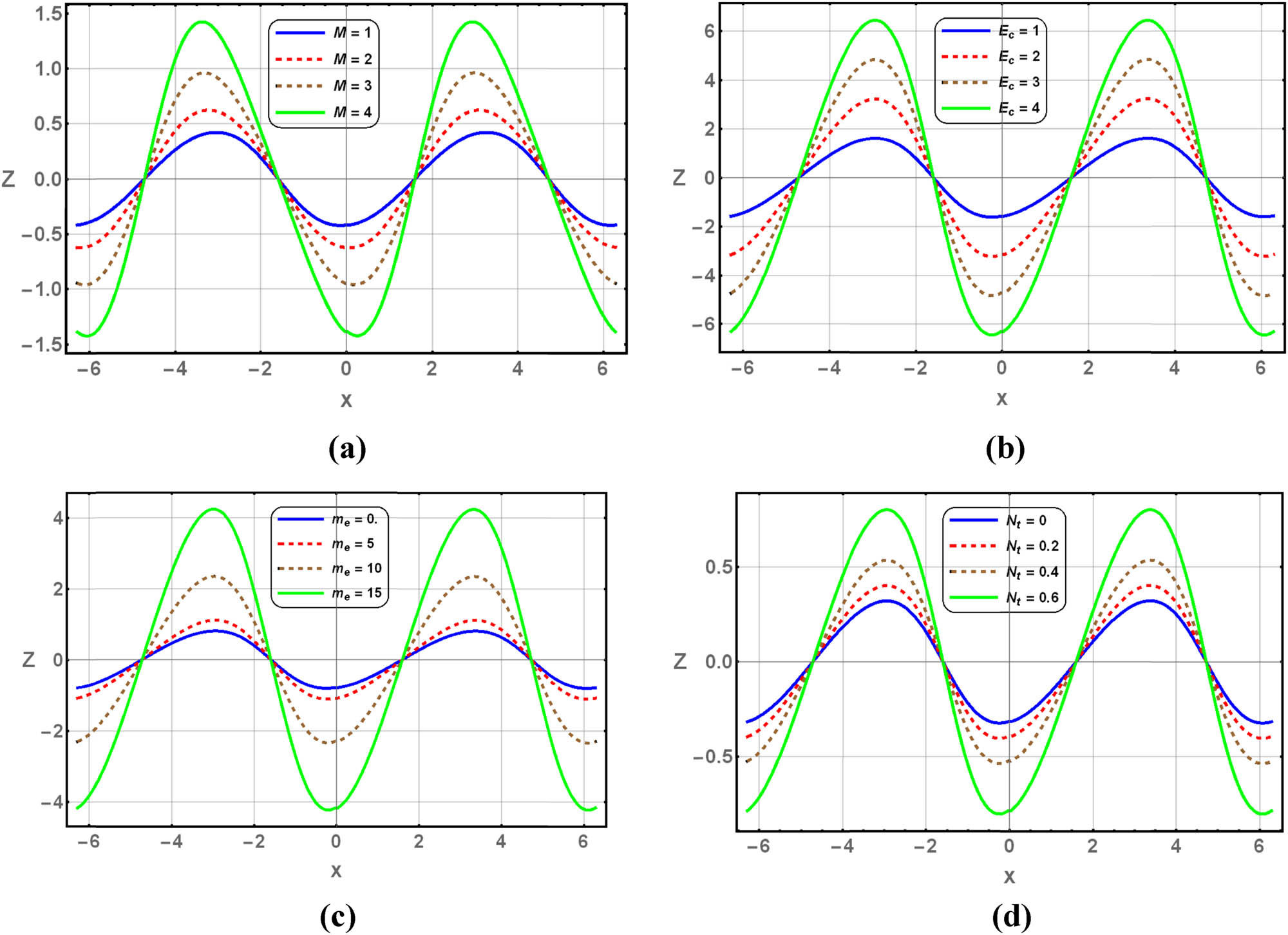
5.5 Microrotation profile

The features and characteristics of various pertinent hydrodynamical flow variables, such as the microrotation slip parameter γ 5 , coupling number N , magnetic field parameter M , and electric field parameter E 1 on dimensionless microrotation speed of the liquid, are shown in Figure 6(a–d). The effect of the microrotation slip parameter γ 5 on the microrotation velocity profile ω ( x , y ) is illustrated in Figure 6(a). It is detected that increasing γ 5 enhances the magnitude of ω ( x , y ) , indicating stronger microrotation near the channel boundaries due to increased slip. Physically, an increment in the microrotation slip variable γ 5 signifies the reduced endurance to spin motion near the channel walls. This allows the fluid particles to rotate more freely at the boundaries, thereby enhancing the microrotation velocity ω ( x , y ) within the domain. The result of this function for the coupling coefficient N on the microrotation characteristic is presented in Figure 6(b). It is perceptibly detected that improving the values of the coupling number N increases the microrotation profile of the fluid. The impact of electromagnetic field parameter M on the microrotation component ω ( x , y ) is shown in Figure 6(c). It was observed that when the parameter associated with the magnetic field increases for a fluid that is micropolar, ω ( x , y ) decreases for a fixed value of y . It is noteworthy to observe that with the increasing number of E 1 , the microrotation profile ω ( x , y ) decreases at the end of the channel, which is shown in Figure 6(d). The accelerating body force is introduced by the electric field that is produced and acts in the applied electrical field. The forward momentum of the boundary layer thickens, and the boundary layer movement is accelerated by this body force, also referred to as the Lorentz force. As a consequence, the microrotation velocity decreased near the channel’s ends.

5.6 Heat transfer rates

In Figure 7(a–d), the corresponding changes in the (a) magnetic field parameter M , (b) Eckert number E c , (c) electroosmotic parameter m e , and (d) thermophoresis parameter N t , respectively, at N = 0.6 , G r = 0.1 , N r = 0.2 , R b = 0.4 , M = 0.1 , E 1 = 0.5 , D a = 0.1 , U HS = − 0.06 , m e = 2 , N t = 0.1 , N t = 0.1 , P r = 6.2 , E c = 0.5 , D u = 0.1 , m = 0.5 , S r = 0.1 , S c = 0.1 , γ 1 = 0.1 , γ 2 = 0.3 , γ 3 = 0.5 , γ 4 = 0.2 , γ 5 = 0.4 , P e = 0.5 , and ε = 0.4 display the heat transfer rate Z progression across the whole channel length. In the area where x = 0.32 , it is observable that the rate of thermal transmission increases by a substantial amount. The shearing stresses that are placed on the boundaries of the channel and the geometrical structures of the walls both provide proof that the oscillation of the walls of the channel is the source of periodic vibrations. The findings demonstrated the evolution of thermal transfer rate Z through the entire channel length. In the same context, the findings indicated that M , E c , m e , and N t increase to maximize heat transfer rates. It is possible to draw the conclusion from this fact that the heat that is produced by viscous dissipation as a result of the viscosity of the fluid increases, and the conduction of heat decreases as the value of the viscous dissipation parameter increases. Consequently, the rate of heat transfer via the sides of the channels might be controlled by these factors due to their influence.

5.7 Streamline patterns

In the context of peristalsis fluid flow, a trapping method is a significant additional feature of rheological effectiveness. The propagating bolus structure of this phenomenon may, in certain instances, take the shape of a streamlined organization that is parallel to the boundary walls. They move in the same orientation as peristaltic impulses and are reliant on the wave that has peristaltic characteristics on the boundary sides. They migrate at the same tempo as peristaltic impulses. The characteristics of regurgitation, an increase in vorticity, as well as the strength of blood flow that occurs during peristalsis movements, can be determined. Figure 8(a–d) shows the additionally discovered behavior of trapping. To portray the streamlined configuration for diverse values of the Helmholtz–Smoluchowski velocity U HS , the magnetic field M , micropolar m , and electroosmotic m e , Figure 8(a–d) shows when N = 0.6 , G r = 0.1 , N r = 0.2 , R b = 0.4 , E 1 = 0.5 , D a = 0.1 , N t = 0.1 , P r = 6.2 , E c = 0.5 , D u = 0.1 , S r = 0.1 , S c = 0.1 , γ 1 = 0.1 , γ 2 = 0.3 , γ 3 = 0.5 , γ 4 = 0.2 , γ 5 = 0.4 , P e = 0.5 , and ε = 0.4 . Upon investigation, it has been discovered that streamlining adheres to the geometric configurations for the issue and fills the flow zone. It is possible to see many convection cells in the area of the uneven edges. A representation of the effect that the Helmholtz–Smoluchowski velocity U HS has on the trapped phenomenon is shown in Figure 8(a). Figure 8(a) demonstrates the increase in the volume of the trapping bolus that occurs when the Debye–Hückel parameter, which is responsible for the reduction in the thickness of the EDL, increases for negative values of the Helmholtz–Smoluchowski speed ( U HS = − 2 ) . On the other hand, when the Helmholtz–Smoluchowski velocity is positive ( U HS = 2 ) , the size of the trapped bolus reduces as the value of the Debye–Hückel coefficient increases. The influence of the magnetic field parameter ( M = 1 − 3 ) and the microrotation factor ( m = 1 − 3 ) on trapping is shown in Figure 8(b) and (c). It has been demonstrated that when the micropolar and magnetic field parameters vary from 1 to 3, there are slight changes in the bolus’ size. In addition, the effect of varying the electroosmotic parameter ( m e = 0 − 10 ) on trapping is depicted in Figure 8(d). More trapping boluses are generated when m e is increased from 0 to 10. The inner composition of the flow can be effectively changed by rationally stating different parameters. This will provide designers with substantial influence over the hydromechanical effectiveness of the pumping in customized applications. In real-world implementations, peristaltic pumps can be more silent, flexible, or partially flexible systems composed of a forcefully compressible, adaptable element (dubbed an engineered composite tube) that entirely closes the inside channel, forming a closed-off chamber made up of the moving sides. The closure points, or contractions, are propelled down the channel by wall shrinkages, which are a natural phenomenon.

6 Concluding remarks

In this study, we have developed a novel mathematical model to investigate the peristalsis flow of a micropolar bio-nanofluid, comprehending gyrotactic microorganisms with the combined effects of electroosmotic forces, magnetized fields, viscous dissipations, Joule heating, first-order chemical reactions, and slip boundary conditions. This comprehensive framework addresses an unstudied configuration in the literature and incorporates important microfluidic phenomena, such as thermophoresis, Brownian motion, and chemical reactions. The model reveals how parameters like the electroosmotic velocity, Helmholtz–Smoluchowski speed, and micropolar effects influence the velocity, temperature, concentration, and microorganism distributions. Importantly, the application of slip conditions enhances physical realism and reflects actual microchannel behaviors. The problem’s linked non-linear differential equations are reduced to a multidimensional form using Reynolds numbers that are small and long-wavelength approximations. Because of the intricacy of the outcome’s set of mathematical equations, mathematical modeling has been performed via the computing software program Mathematica by employing the integrated function (parametric NDSolve). The results offer a thorough comprehension of the system’s behavior, which exhibits a significant correlation with the physical characteristics controlling it. In particular, the zeta potential, voltage, and channel shape are found to have a considerable impact on the acceleration of EOF. These discoveries may prove useful in the creation of microfluidic devices suitable for certain uses requiring fine-grained fluid handling. Finally, we discussed how various parameters affect the results. The significant findings are as follows:

The administration of specific pharmaceuticals may be enhanced by using electroosmotic forces to modify the nanofluid during peristalsis movement. This coordinated mobility may facilitate the exact delivery of drugs to certain physiological regions or cells.
Thermal and mass transport phenomena are highly sensitive to slip boundary conditions. For instance, thermal and concentration slip enhance energy and species diffusion, influencing nanoparticle and microorganism distributions.
Regulated buoyant forces may be used in biological processes to manipulate the behavior of nanoparticles in blood-based fluids. For instance, it may influence the distribution and circulation of therapeutic nanomaterials in drug delivery systems.
Electroosmotic forces play a dominant role in enhancing flow transport; increasing the zeta potential and electric field intensity significantly boosts the axial flow and nanoparticle convection.
The density of motile bacteria exhibits contrasting results with increasing levels of the Brownian movement variable and the thermophoretic variable.
The Helmholtz–Smoluchowski velocity emerges as a critical parameter in tuning both the fluid velocity and particle concentration profiles, particularly near the channel center.
Trapping phenomena are notably affected by the electroosmotic parameters, revealing possibilities for controlled transport and targeted delivery in bio-microfluidic systems.
The results of this study exhibit a strong correlation with the body of literature already in circulation [47,48].
The micropolar effects, including microrotation and spin viscosity, subtly influence the flow near the walls but have a limited effect at the core region, offering fine control over wall-bound layer dynamics.
The theoretical results may find practical applications in physiological flows and commercial applications involving electroosmosis-driven peristaltic transport subjected to microrotation of fluid particles.

7 Future directions and limitations

This work can be developed further in several ways. The significance of biomedical engineering has been strengthened by its reliance on curvature effects. It is also important to note the application of different rheological concepts and the ciliated wall effects, along with the pushing of bacterial cells and spermatozoa. These practical studies will contribute to the development of more advanced nanomagnetic and electric microrobots. The current analysis relies on several simplifying assumptions, such as the long wavelength, low Reynolds number, and the Debye–Hückel approximation, which limits its applicability to low-potential, slow-flow regimes. The model also considers constant wall properties and diminished first-order chemical reactions. Although these assumptions were required for tractability, they may not fully capture the complexity of actual bio-microfluidic systems. Future work could target optimization of flow rate by tuning electrokinetic and geometric parameters. Additionally, a sensitivity analysis is recommended in future investigations to identify the most influential parameters affecting the system behavior and optimize design considerations accordingly.

Acknowledgments

The authors extend their appreciation to the Deanship of Scientific Research at Northern Border University, Arar, KSA for funding this research work through the project number NBU-FFR-2025-3021-08. The authors are thankful to the Deanship of Graduate Studies and Scientific Research at University of Bisha for supporting this work through the Fast-Track Research Support Program.

Funding information: The Deanship of Scientific Research at Northern Border University, Arar, KSA for funding this research work through the project number NBU-FFR-2025-3021-08. The authors are thankful to the Deanship of Graduate Studies and Scientific Research at University of Bisha for supporting this work through the Fast-Track Research Support Program.
Author contributions: Conceptualization: EME, SAH, and NTME; data curation: AMA and KhL; formal analysis: EME, SAH, and MRE; investigation: NTME, KhL, and MRE; methodology: SAH and AMA; project administration: MRE; supervision: NTME; validation: EME, NTME, and MRE; visualization: SAH and KhL; writing – original draft: SAH, AMA, and KhL; writing – review and editing: EME, AMA, and MRE. All authors have accepted responsibility for the entire content of this manuscript and approved its submission.
Conflict of interest: The authors state no conflict of interest.
Data availability statement: All data generated or analyzed during this study are included in this published article.

References

[1] Choi SU, Eastman JA. Enhancing thermal conductivity of fluids with nanoparticles. Argonne, IL (United States): Argonne National Laboratory (ANL); 1995.Search in Google Scholar

[2] Buongiorno J. Convective transport in nanofluids. ASME J Heat Transf. 2006;128(3):240–50.10.1115/1.2150834Search in Google Scholar

[3] Leong KY, Saidur R, Kazi S, Mamun A. Performance investigation of an automotive car radiator operated with nanofluid-based coolants. Appl Therm Eng. 2010;30(17–18):2685–92.10.1016/j.applthermaleng.2010.07.019Search in Google Scholar

[4] Mustafa M, Hina S, Hayat T, Alsaedi A. Influence of wall properties on the peristaltic flow of a nanofluid: analytic and numerical solutions. Int J Heat Mass Transf. 2012;55(17–18):4871–7.10.1016/j.ijheatmasstransfer.2012.04.060Search in Google Scholar

[5] Kothandapani M, Prakash J. Effect of radiation and magnetic field on peristaltic transport of nanofluids through a porous space in a tapered asymmetric channel. J Magn Magn Mater. 2015;378:152–63.10.1016/j.jmmm.2014.11.031Search in Google Scholar

[6] Hayat T, Nisar Z, Yasmin H, Alsaedi A. Peristaltic transport of nanofluid in a compliant wall channel with convective conditions and thermal radiation. J Mol Liq. 2016;220:448–53.10.1016/j.molliq.2016.04.080Search in Google Scholar

[7] Abbasi F, Gul M, Shehzad S. Effectiveness of temperature-dependent properties of Au, Ag, Fe3O4, Cu nanoparticles in peristalsis of nanofluids. Int Commun Heat Mass Transf. 2020;116:104651.10.1016/j.icheatmasstransfer.2020.104651Search in Google Scholar

[8] Abd-Alla A, Thabet EN, Bayones F. Numerical solution for MHD peristaltic transport in an inclined nanofluid symmetric channel with porous medium. Sci Rep. 2022;12(1):3348.10.1038/s41598-022-07193-5Search in Google Scholar PubMed PubMed Central

[9] Tahir M, Ahmad A, Shehzad SA. Study of pseudoplastic and dilatant behavior of nanofluid in peristaltic flow: Reiner-Philippoff models. Chin J Phys. 2022;77:2371–88.10.1016/j.cjph.2022.04.001Search in Google Scholar

[10] Nisar Z, Hayat T, Alsaedi A, Momani S. Peristaltic flow of chemically reactive Carreau-Yasuda nanofluid with modified Darcy’s expression. Mater Today Commun. 2022;33:104532.10.1016/j.mtcomm.2022.104532Search in Google Scholar

[11] Nisar Z, Hayat T, Alsaedi A, Momani S. Mathematical modelling for peristaltic flow of fourth‐grade nanoliquid with entropy generation. Z Angew Math Mech. 2024;104(1):e202300034.10.1002/zamm.202300034Search in Google Scholar

[12] Ahmed SE, Arafa AA, Hussein SA. Hydrothermal dissipative nanofluid flow over a stretching Riga plate with heat and mass transmission and shape effects. J Therm Anal Calorim. 2024;149(10):4855–72.10.1007/s10973-024-13061-3Search in Google Scholar

[13] Latham TW. Fluid motions in a peristaltic pump. Cambridge (MA): Massachusetts Institute of Technology; 1966.Search in Google Scholar

[14] Shapiro AH, Jaffrin MY, Weinberg SL. Peristaltic pumping with long wavelengths at low Reynolds number. J Fluid Mech. 1969;37(4):799–825.10.1017/S0022112069000899Search in Google Scholar

[15] Srinivas S, Gayathri R, Kothandapani M. The influence of slip conditions, wall properties and heat transfer on MHD peristaltic transport. Comput Phys Commun. 2009;180(11):2115–22.10.1016/j.cpc.2009.06.015Search in Google Scholar

[16] Tripathi D. A mathematical model for the peristaltic flow of chyme movement in small intestine. Math Biosci. 2011;233(2):90–7.10.1016/j.mbs.2011.06.007Search in Google Scholar PubMed

[17] Sarkar B, Das S, Jana R, Makinde O. Magnetohydrodynamic peristaltic flow of nanofluids in a convectively heated vertical asymmetric channel in presence of thermal radiation. J Nanofluids. 2015;4(4):461–73.10.1166/jon.2015.1169Search in Google Scholar

[18] Reddy MG, Makinde O. Magnetohydrodynamic peristaltic transport of Jeffrey nanofluid in an asymmetric channel. J Mol Liq. 2016;223:1242–8.10.1016/j.molliq.2016.09.080Search in Google Scholar

[19] Reddy KV, Reddy MG, Makinde OD. Heat and mass transfer of a peristaltic electro-osmotic flow of a couple stress fluid through an inclined asymmetric channel with effects of thermal radiation and chemical reaction. Period Polytech Mech Eng. 2021;65(2):151–62.10.3311/PPme.16760Search in Google Scholar

[20] Priam SS, Nasrin R. Numerical appraisal of time-dependent peristaltic duct flow using Casson fluid. Int J Mech Sci. 2022;233:107676.10.1016/j.ijmecsci.2022.107676Search in Google Scholar

[21] Ahmed SE, Arafa AA, Hussein SA. Viscous dissipation and Joule heating in case of variable electrical conductivity Carreau–Yasuda nanofluid flow in a complex wavy asymmetric channel through porous media. Mod Phys Lett B. 2024;38(36):2450369.10.1142/S021798492450369XSearch in Google Scholar

[22] Sayed AAM, Abo-Elkhair RE, Elsaid EM. Improving the rheological behavior of magnetiz couple stress Buongiorno’s nanofluid through resilient wavy channel with curvature effect: Nonlinear analysis. Chin J Phys. 2024;89:1508–37.10.1016/j.cjph.2024.04.017Search in Google Scholar

[23] Li H, Wei S, Qing C, Yang J. Discussion on the position of the shear plane. J Colloid Interface Sci. 2003;258(1):40–4.10.1016/S0021-9797(02)00077-2Search in Google Scholar

[24] Ghosal S. Fluid mechanics of electroosmotic flow and its effect on band broadening in capillary electrophoresis. Electrophoresis. 2004;25(2):214–28.10.1002/elps.200305745Search in Google Scholar PubMed

[25] Chakraborty S. Augmentation of peristaltic microflows through electro-osmotic mechanisms. J Phys D Appl Phys. 2006;39(24):5356.10.1088/0022-3727/39/24/037Search in Google Scholar

[26] Dutta P, Beskok A. Analytical solution of combined electroosmotic/pressure driven flows in two-dimensional straight channels: finite Debye layer effects. Anal Chem. 2001;73(9):1979–86.10.1021/ac001182iSearch in Google Scholar PubMed

[27] Liakopoulos AC. Darcy’s coefficient of permeability as symmetric tensor of second rank. Hydrol Sci J. 1965;10(3):41–8.10.1080/02626666509493405Search in Google Scholar

[28] Ramesh K, Devakar M. Effect of heat transfer on the peristaltic transport of a MHD second grade fluid through a porous medium in an inclined asymmetric channel. Chin J Phys. 2017;55(3):825–44.10.1016/j.cjph.2016.10.028Search in Google Scholar

[29] Ranjit N, Shit G, Tripathi D. Joule heating and zeta potential effects on peristaltic blood flow through porous micro vessels altered by electrohydrodynamic. Microvasc Res. 2018;117:74–89.10.1016/j.mvr.2017.12.004Search in Google Scholar PubMed

[30] Noreen S, Tripathi D. Heat transfer analysis on electroosmotic flow via peristaltic pumping in non-Darcy porous medium. Therm Sci Eng Prog. 2019;11:254–62.10.1016/j.tsep.2019.03.015Search in Google Scholar

[31] Lodhi RK, Ramesh K. Comparative study on electroosmosis modulated flow of MHD viscoelastic fluid in the presence of modified Darcy’s law. Chin J Phys. 2020;68:106–20.10.1016/j.cjph.2020.09.005Search in Google Scholar

[32] Reddappa B, Parandhama A, Sreenadh S. Peristaltic transport of conducting Williamson fluid in a porous channel. J Math Comput Sci. 2019;10(2):277–88.Search in Google Scholar

[33] Platt JR. Bioconvection patterns in cultures of free-swimming organisms. Science. 1961;133(3466):1766–7.10.1126/science.133.3466.1766Search in Google Scholar PubMed

[34] Pedley TJ, Hill N, Kessler JO. The growth of bioconvection patterns in a uniform suspension of gyrotactic micro-organisms. J Fluid Mech. 1988;195:223–37.10.1017/S0022112088002393Search in Google Scholar PubMed

[35] Sampath Kumar P, Gireesha B, Mahanthesh B, Chamkha AJ. Thermal analysis of nanofluid flow containing gyrotactic microorganisms in bioconvection and second order slip with convective condition. J Therm Anal Calorim. 2019;136:1947–57.10.1007/s10973-018-7860-0Search in Google Scholar

[36] Eldabe N, Gabr M, Hussein SA. Numerical treatment for the boundary layer flow of Sutterby nanofluid through porous medium with planktonic microorganisms over a stretching Riga cylindrical tube. Int J Ambient Energy. 2024;45(1):2345251.10.1080/01430750.2024.2345251Search in Google Scholar

[37] Hussein SA, Arafa AA, Elshekhipy A, Hassan Almalki N, AL-Essa L, Akbar Y. Radiative and dissipative MHD Eyring–Powell nanofluid bioconvective flow through peristaltic waves in the presence of bilateral chemical reaction with Arrhenius activation energy: entropy optimization. Numer Heat Transf A Appl. 2023;83(1):1–27.Search in Google Scholar

[38] Alqarni AJ, Elsaid EM, Al Qarni AA, Mekheimer KS, Abo-Elkhair RE, Abdel-Wahed MS. Exploration of bioconvection flow for biological fluid with planktonic microorganism and thermal radiation: Drug carriers for tumor cells. Mod Phys Lett B. 2024;38(36):2450505.10.1142/S0217984924505055Search in Google Scholar

[39] Ahmed SE, Arafa AA, Hussein SA. MHD Ellis nanofluids flow around rotating cone in the presence of motile oxytactic microorganisms. Int Commun Heat Mass Transf. 2022;134:106056.10.1016/j.icheatmasstransfer.2022.106056Search in Google Scholar

[40] Abd-Alla A, Abo-Dahab S, Thabet EN, Abdelhafez M. Heat and mass transfer for MHD peristaltic flow in a micropolar nanofluid: mathematical model with thermophysical features. Sci Rep. 2022;12(1):21540.10.1038/s41598-022-26057-6Search in Google Scholar PubMed PubMed Central

[41] Noreen S, Batool S, Tripathi D. Electroosmosis and peristaltic mechanism in a symmetric channel flow. Microfluid Nanofluid. 2024;28(3):15.10.1007/s10404-024-02712-4Search in Google Scholar

[42] Waheed S, Noreen S, Hussanan A. Study of heat and mass transfer in electroosmotic flow of third order fluid through peristaltic microchannels. Appl Sci. 2019;9(10):2164.10.3390/app9102164Search in Google Scholar

[43] Ramesh K, Prakash J. Thermal analysis for heat transfer enhancement in electroosmosis-modulated peristaltic transport of Sutterby nanofluids in a microfluidic vessel. J Therm Anal Calorim. 2019;138:1311–26.10.1007/s10973-018-7939-7Search in Google Scholar

[44] Yasmin H, Iqbal N. Convective mass/heat analysis of an electroosmotic peristaltic flow of ionic liquid in a symmetric porous microchannel with soret and dufour. Math Probl Eng. 2021;2021(1):2638647.10.1155/2021/2638647Search in Google Scholar

[45] Choudhari R, Ramesh K, Tripathi D, Vaidya H, Prasad KV. Heat transfer and electroosmosis driven MHD peristaltic pumping in a microchannel with multiple slips and fluid properties. Heat Transf. 2022;51(7):6507–27.10.1002/htj.22602Search in Google Scholar

[46] Hussain A, Saddiqa A, Riaz MB, Martinovic J. A comparative study of peristaltic flow of electro-osmosis and MHD with solar radiative effects and activation energy. Int Commun Heat Mass Transf. 2024;156:107666.10.1016/j.icheatmasstransfer.2024.107666Search in Google Scholar

[47] Hussein SA, Ahmed SE, Arafa AA. Electrokinetic peristaltic bioconvective Jeffrey nanofluid flow with activation energy for binary chemical reaction, radiation and variable fluid properties. Z Angew Math Mech. 2023;103(1):e202200284.10.1002/zamm.202200284Search in Google Scholar

[48] Jhorar R, Tripathi D, Bhatti M, Ellahi R. Electroosmosis modulated biomechanical transport through asymmetric microfluidics channel. Indian J Phys. 2018;92:1229–38.10.1007/s12648-018-1215-3Search in Google Scholar

[49] Kotnurkar AS, Giddaiah S. Bioconvection peristaltic flow of nano Eyring–Powell fluid containing gyrotactic microorganism. SN Appl Sci. 2019;1(10):1276.10.1007/s42452-019-1281-ySearch in Google Scholar

[50] Tang G, Li X, He Y, Tao W. Electroosmotic flow of non-Newtonian fluid in microchannels. J Non-Newton Fluid Mech. 2009;157(1–2):133–7.10.1016/j.jnnfm.2008.11.002Search in Google Scholar

[51] Noreen S. Mixed convection peristaltic flow of third order nanofluid with an induced magnetic field. PLoS One. 2013;8(11):e78770.10.1371/journal.pone.0078770Search in Google Scholar PubMed PubMed Central

[52] Hussein SA. Simulating and interpretation of MHD peristaltic transport of dissipated Eyring–Powell nanofluid flow through vertical divergent/nondivergent channel. Numer Heat Transf A Appl. 2023;84(10):1124–48.10.1080/10407782.2023.2171928Search in Google Scholar

[53] Hussein SA. Numerical simulation for peristaltic transport of radiative and dissipative MHD Prandtl nanofluid through the vertical asymmetric channel in the presence of double diffusion convection. Numer Heat Transf B Fundam. 2024;85(4):385–411.10.1080/10407790.2023.2235886Search in Google Scholar

[54] Ali N, Hayat T. Peristaltic flow of a micropolar fluid in an asymmetric channel. Comput Math Appl. 2008;55(4):589–608.10.1016/j.camwa.2007.06.003Search in Google Scholar

[55] Hayat T, Khan A, Bibi F, Farooq S. Activation energy and non-Darcy resistance in magneto peristalsis of Jeffrey material. J Phys Chem Solids. 2019;129:155–61.10.1016/j.jpcs.2018.12.044Search in Google Scholar

Received: 2025-04-18

Revised: 2025-07-08

Accepted: 2025-07-25

Published Online: 2025-09-20

This work is licensed under the Creative Commons Attribution 4.0 International License.

Articles in the same Issue

https://doi.org/10.1515/phys-2025-0208

Keywords for this article

micropolar nanofluid; peristaltic waves; electroosmotic flow; magnetic field; gyrotactic bacteria; slip conditions; porous medium; Soret and Dufour effects

Creative Commons

BY 4.0