A new family of Poisson-exponential distributions with applications to cancer data and glass fiber reliability

Bahady I. Mohammed; Oluwafemi Samson Balogun; Mahmoud E. Bakr; Yusra A. Tashkandy

doi:10.1515/phys-2025-0241

Article Open Access

A new family of Poisson-exponential distributions with applications to cancer data and glass fiber reliability

Bahady I. Mohammed , Oluwafemi Samson Balogun , Mahmoud E. Bakr and Yusra A. Tashkandy

Published/Copyright: December 4, 2025

Published by

Become an author with De Gruyter Brill

Submit Manuscript Author Information Explore this Subject

From the journal Open Physics Volume 23 Issue 1

Abstract

Towards the end of the 20th century, statisticians were keen to create new distribution families that would meet the rapid advancements in modeling and application domains while also getting around constraints on certain distributions. In this study, a new family is proposed for adding one parameter to a continuous distribution by using countable mixture of PE distribution. Some attributes such as the probability density function extreme stability, and the hazard rate function of the new family are provided. As a member of the purpose family, a Weibull distribution illustration is presented. Poisson exponential Weibull (PE-W) characteristics such as compound, moments, skewness, kurtosis, and others are derived. Using both complete and censored data sets as well as simulated experiments, the maximum likelihood estimation of PE-W parameters was examined. Further, to illustrate the value of the PE-W distribution compared to other commonly used distributions, an analysis is carried out on actual and censored data sets that represent the breaking stress of carbon fibers and liver (lung) cancer.

Keywords: Poisson exponential; Poisson exponential Weibull model; mean inactivity time; censored and complete data; model selections; p-p plot

1 Introduction

One of the significant research issues that is still very much alive in statistics is the topic of creating and expanding families of probability continuous distributions. A number of factors contribute to this, including the need for new probabilistic distributions to better describe each phenomenon as the amount of data available for analysis grows at an accelerating rate and the ease with which the computational and analytical tools found in programming software like R, Maple, and Mathematica can handle the challenges associated with computing special functions in these extended distributions. For example, Marshall and Olkin [1], AL-Hussaini and Gharib [2], AL-Hussaini and Ghitany [3], Alzaatreh et al. [4], Guitany et al. [5], Cordeiro and de Castro [6], Bourguignon et al. [7], Brito et al. [8], Gharib et al. [9], and Chipepa et al. [10]. These new models offer increased usefulness and flexibility. These categories of applications include financial and insurance applications, as well as applications in hydrology, engineering, economics, and medicine see Alsadat et al. [11], Dina et al. [12], Ahmed et al. [13] and Aljohani [14].

The Poisson distribution is frequently used to model count data sets. Nevertheless, overdispersed data sets cannot be handled by the Poisson distribution. When the variation is greater than the mean, overdispersion is present. In order to provide alternate models for highly distributed count data, some researchers have created mixed Poisson distributions. In order to provide alternative models for over dispersed count data, numerous researchers have created mixed-Poisson distributions, such as Mahmoudi and Zakerzadeh [15], Bereta et al. [16], Bhati et al. [17], Miao et al. [18], Altun [19], 20]. Fazal and Bashir [21] obtained The Poisson exponential (PE) distribution which is a perfect modification of the Poisson distribution and the Lindley distribution, and it is utilized to model biological and traffic data sets.

In this paper, we have provided the new family of countable mixes with the PE distribution. This family possesses a stability property, meaning that if the procedure is used twice, no new results are obtained. In addition, one member of this family provides an illustration of the Weibull survival function. Researchers such as Estela et al. [22], Ana Percontini et al. [23], Cordeiro and Lemonte [24], Muhammad Bilal et al. [25], Kumaraswamy and Bhatra Charyulu [26], and Adam Braima et al. [27] have extended the Weibull distribution because of its significance in modeling and applied fields.

This paper discusses a new family based on the PE with generalized failure rate function. Section 3 presents the new distribution Poisson exponential Weibull (PE-W) model and its properties. Section 4 outlines an PE-W (γ, θ, λ) characteristics as, compounding, moment generating function (MGF), mean residual life (MRL) and mean inactivity time (MIT). Section 5 contains the estimating PE-W parameters. Section 6 evaluates the performance of maximum likelihood using Monte Carlo simulations. In Section 7 the methodology is illustrated in a real data set. There are a few closing remarks given in Section 8.

2 The PE family

In this section, we propose a new family of PE distribution. We derive survival function (SF), density and hazard rate functions of the new family.

Suppose that F ̄ x is the SF and for j = 1,2 , … , x ∈ R , the components F ̄ j x are given by:

F ̄ j x = F ̄ j x , j = 1,2 , … , − ∞ < x < ∞ .

then,

(1) G ̄ x = ∑ j = 1 ∞ π j F ̄ j x ,

where, F ̄ x is the SF of a random variable (RV), π _j ≥ 0, for j = 1, 2, … and ∑ j = 1 ∞ π j = 1 , In this case, G ̄ x is called countable mixture.

The use of mixtures to obtain flexible families of densities has a long history, especially in the univariate case. The advantages of the mixture’s mechanism are diverse. The new classes of distributions obtained by mixing are more flexible than the original, over dispersed with tails larger than the original distribution and often providing better fits see Fisher [28] Teicher [29].

If we consider π _j is to be the PE distribution with parameter ( θ ), where

(2) π j = θ 1 + θ j , θ > 0 , j = 1,2 … ,

To model counting data, the PE distribution combines Poisson and exponential distributions. Then the compound (mixture) distribution G ̄ x of F ̄ j x is:

G ̄ x = ∑ j = 1 ∞ π j F ̄ x j = ∑ j = 1 ∞ θ 1 + θ j F ̄ j x = θ ∑ j = 1 ∞ F ̄ x 1 + θ j ,

using the fact, ∑ j = 1 ∞ F ̄ x 1 + θ j = F ̄ x 1 + θ − F ̄ x = F ̄ x θ + F x , then

(3) G ̄ x = θ F ̄ x θ + F x , θ > 0 , − ∞ < x < ∞

where, F x is the cumulative distribution function (CDF) of X.

And probability density function (PDF):

(4) g x = − d d x G ̄ x = − d d x θ F ̄ x θ + F x − 1 = θ f x θ + 1 θ + F x 2 = θ f x θ + 1 θ + F x 2

The corresponding hazard rate function (HRF), which is the expected failure rate of an item at a given age, used in survival analysis to assess the likelihood of survival over time and given by:

(5) r x = g x G ̄ x = f x F ̄ x θ θ + 1 θ + F x = h x θ θ + 1 θ + F x .

Clearly, lim x → 0 r x = θ + 1 lim x → 0 h x and lim x → ∞ r x = θ lim x → ∞ h x

Theorem 1:

The parametric family of G ̄ x = θ F ̄ x θ + F x is PE extreme stable.

Proof

Let X _i, i = 1, 2, …, n to be independent identically distributed (i.i.d), N is independent of the X _i’s with PE distribution and if:

U N = min x 1 , x 2 , … , x N , V N = max x 1 , x 2 , … , x N ,

then

G ̄ x = Pr U N > x = Pr x 1 > x 1 , x 2 > x 2 , … , x N > x N = ∑ n = 1 ∞ F ̄ n x θ 1 + θ n = θ F ̄ x θ + F x , − ∞ < x < ∞ ,

Hence U _N is PE minimum stable, and

H x = Pr V N < x = Pr x 1 < x 1 , x 2 < x 2 , … , x N < x N = ∑ n = 1 ∞ F n x θ 1 + θ n = θ F x θ + F ̄ x ,

so that,

H ̄ x = θ F ̄ x θ + F x , − ∞ < x < ∞ .

Hence V _N is PE maximum stable, therefore, the family of PE distributions with G ̄ x is PE extreme stable.

An illustrative example of this class is provided where F ̄ is the SF of the Weibull distribution, which is one of the most well-known distributions for life data analysis and modeling in applied, medical, and engineering sciences, as well as reliability applications to simulate failure times.

3 PE-W model

A RV X is given the Weibull distribution, represented as X ∼ W(λ, γ), if its SF and PDF are as follows:

F ̄ x = e − λ x γ , λ , γ , x > 0 , λ , γ > 0 ,

and

f x = γ λ x γ − 1 e − λ x γ , x > 0 , λ , γ > 0 .

where, λ is the scale parameter and γ is the shape parameter.

The corresponding HRF takes the following form:

h x = γ λ x γ − 1 , x > 0 , λ , γ > 0 .

Clearly, that the h(x) has three different forms: constant when γ = 1 and decreasing (increases) when γ < 1 (γ > 1).

The PE-W distribution’s SF and PDF have the following forms:

(6) G ̄ x = θ e − λ x γ 1 + θ − e − λ x γ = θ − 1 + e x γ λ 1 + θ ,

where, θ , λ are scale parameters and γ the shape parameter, and

(7) g x = γ θ 1 + θ λ x − 1 + γ e x γ λ − 1 + e x γ λ 1 + θ 2

Clearly, lim x → ∞ g x = 0 for γ > 0 and lim x → 0 g x = 0 for γ > 1.

A selection of parameter values for the PE-W distribution’s PDF plots are shown in Figures 1 and 2.

Figure 1:

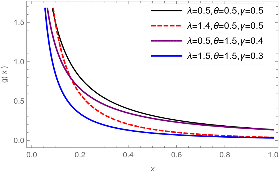
Decreasing PE-W PDF for values γ, λ and θ.

Figure 2:

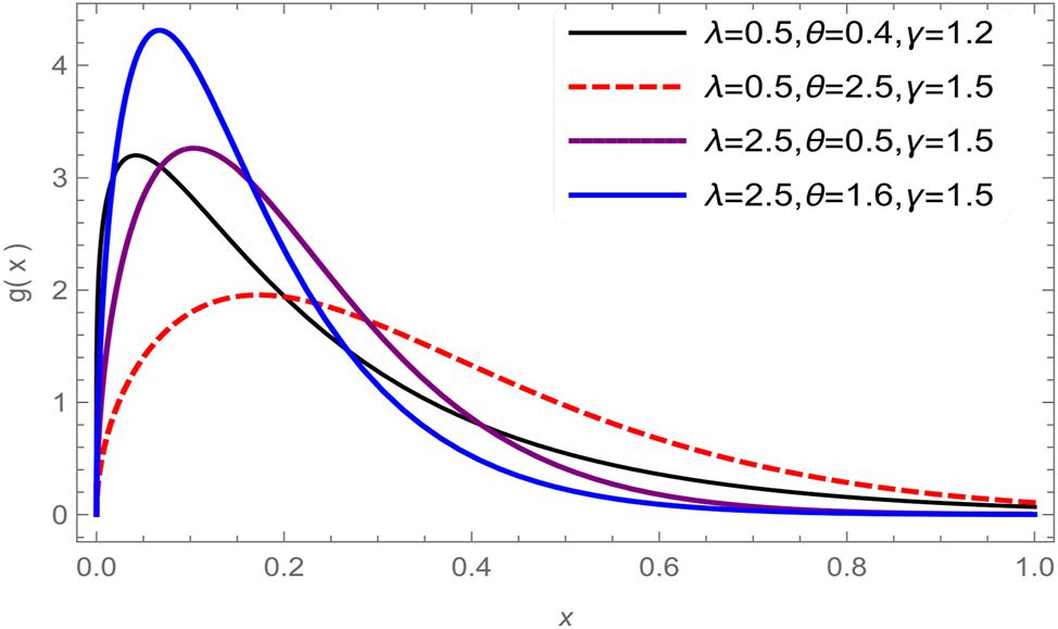
Unimodal PE-W PDF for values γ, λ and θ.

Figures 1 and 2: show that the g(x) given by Eq. (7) for the selected values of γ, λ and θ. In Figure 1, γ < 1 showing that g(x) is decreasing. In Figure 2, γ > 1 showing that g(x) is increasing-decreasing.

The corresponding HRF of PE-W distribution is:

(8) r x = e x γ λ x − 1 + γ γ 1 + θ λ − 1 + e x γ λ 1 + θ

Clearly, lim x → ∞ r x = ∞ for γ > 1 and lim x → 0 r x = 0 for γ > 1

The HRF plots of the PE-W distribution with a range of parameters values are displayed in Figures 3 and 4.

Figure 3:

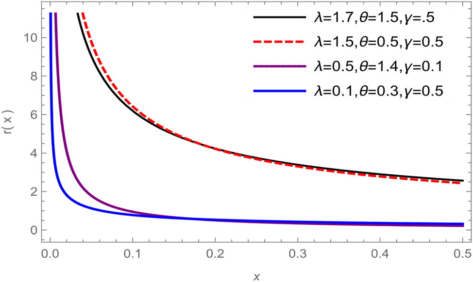
Decreasing PE-W HRF for values γ, λ and θ.

Figure 4:

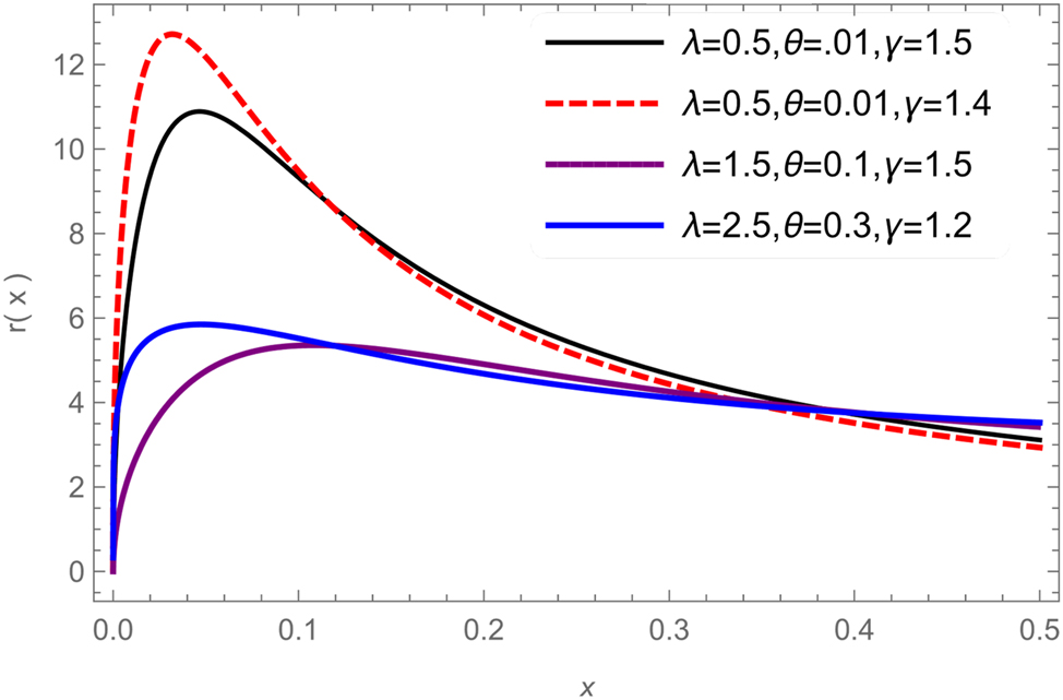
Unimodal PE-W HRF for values γ, λ and θ.

Figures 3 and 4: show that the r(x) given by Eq. (8) for the selected values of γ, λ and θ. In Figure 3, γ < 1 showing that r(x) is decreasing. In Figure 4, γ > 1 showing that r(x) is increasing-decreasing.

4 PE-W (γ, θ, λ) characteristics

4.1 Compounding

Let G ̄ x β be the conditional SF of a continuous RV X given a continuous RV β. Let β follows a distribution with the PDF m β . A distribution with the SF:

G ̄ x = ∫ − ∞ ∞ G ̄ x β m β d β , − ∞ < x < ∞

is called a compound distribution with mixing density m β . One helpful method for obtaining a new class of distributions in terms of preexisting ones is the compound distribution. The following theorem demonstrates that the PE-W distribution can be generated through the application of the following theorem.

Theorem 2:

Let, G ̄ x β = exp β e − λ x γ − 1 − λ x γ and β have the PDF m β = θ e − θ β . Then, the PE-W (λ, γ,θ) distribution characterizes the compound distribution of X.:

Proof

G ̄ x = ∫ 0 ∞ G ̄ x β m β d β G ̄ x = θ ∫ 0 ∞ exp − β 1 − e − λ x γ + θ d β = θ e − λ x γ 1 − e − λ x γ + θ = θ − 1 + 1 + θ e λ x γ

This is the SF of the PE-W (λ, γ, θ) distribution.

4.2 The rth moment and quantiles of PE-W model

For the PE-W (γ, θ, λ) distribution, the rth moment E x r , r ≥ 1 , is:

E x r = r ∫ 0 ∞ x r − 1 G ̄ x d x = r ∫ 0 ∞ x r − 1 θ − 1 + e x γ λ 1 + θ d x = r θ 1 + θ ∫ 0 ∞ x r − 1 e − λ x γ 1 − e − λ x γ 1 + θ d x

Let, y = λx ^γ then

E x r = r θ 1 + θ γ λ r γ − 1 ∫ 0 ∞ y r γ − 1 e − y 1 − e − y 1 + θ d y E x r = r θ 1 + θ γ λ r γ − 1 ∫ 0 ∞ ∑ n = 0 ∞ ∑ m = 0 ∞ y r γ − 1 − 1 n × y n n ! e − y 1 + θ m d y = r θ 1 + θ m + 1 γ λ r γ − 1 ∑ n = 0 ∞ ∑ m = 0 ∞ ( − 1 ) n n ! × ∫ 0 ∞ y n + r γ − 1 e − my d y = r θ 1 + θ m + 1 γ λ r γ − 1 × ∑ n = 0 ∞ ∑ m = 0 ∞ ( − 1 ) n n ! m − r + n γ γ Γ n + r γ .

where Γ is gamma function.

The PE-W model’s qth quantile is:

Q q = log 1 + θ − q 1 + θ 1 − q 1 γ λ , 0 ≤ q ≤ 1 ,

Specifically, the PE-W model’s median is:

m e d i a n x = log 2 θ + 1 1 + θ 1 γ λ .

As a result, we can use metrics based on certain quartiles to examine the structure of the PE-W model.

To demonstrate how the scale parameter θ and shape parameters γ and λ affect the new distribution’s skewness and kurtosis, we look at quantile-based metrics. The traditional kurtosis measure’s drawbacks are widely recognized. This measure becomes uninformative just when it should be because it is infinite for many heavy-tailed distributions. The lack of traditional kurtosis for a large number of generalized distributions was, in fact, the driving force behind our decision to employ quantile-based metrics. According to Kenney & Keeping [30] and Moors kurtosis [31] the Skewness (Sk) and kurtosis (Ku) are:

S k = Q 3 / 4 − 2 Q 1 / 2 + Q 1 / 4 Q 3 / 4 − Q 1 / 4 , K u = Q 7 / 8 − Q 5 / 8 − Q 3 / 8 + Q 1 / 8 Q 6 / 8 − Q 2 / 8 .

5 illustrates how the Sk and Ku depend on the parameters by displaying the Bowley skewness and Moors kurtosis for several values of the parameters.

Figure (5.a):

Displays the PE-W distribution’s Sk as a function of a (θ) for specific values of λ and θ (for certain values of γ, λ).

Figure (5.b):

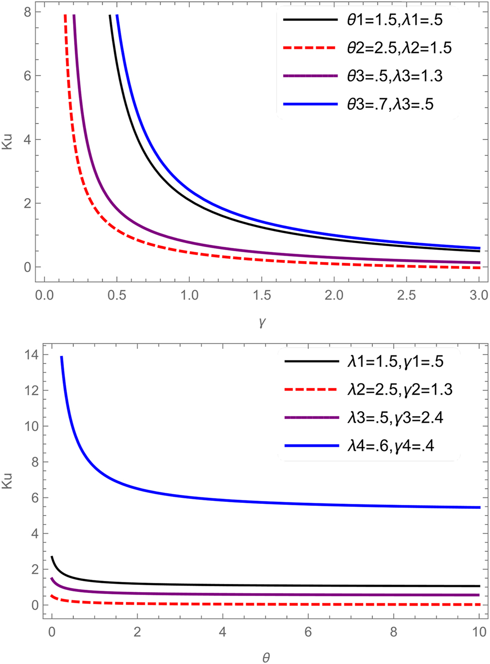
Displays the Ku of the PE-W distribution as a function of a (θ) for specific values of λ and θ (for certain values of γ, λ).

Figure 5: Shows how the scale θ and the shape factors γ and λ affect the skewness and kurtosis of the PE-W distribution. In figure (5.a), Skewness decreases with increasing θ, suggesting that higher θ lead to more symmetric distributions. In figure (5.b), kurtosis decreases with increasing γ in all configurations, indicating that the distributions become less heavy-tailed as the coupling strength increases.

4.3 MGF and MRL of PE-W (γ, θ, λ) distribution

The MGF for the PE-W (γ, θ, λ) distribution is:

M t = ∫ 0 ∞ e t x γ θ 1 + θ λ x − 1 + γ e x γ λ − 1 + e x γ λ 1 + θ 2 d x = γ θ 1 + θ λ ∫ 0 ∞ e t x x − 1 + γ e x γ λ − 1 + e x γ λ 1 + θ 2 d x = γ θ λ ∫ 0 ∞ x − 1 + γ e t x − 1 + e x γ λ 1 + θ 1 1 − e − λ x γ 1 + θ d x

using the fact, 1 1 − e − λ x γ 1 + θ = ∑ m 1 = 0 ∞ e − λ x γ 1 + θ m 1 , then

M t = γ θ λ 1 + θ ∫ 0 ∞ x − 1 + γ e t x e − x γ λ 1 − e − λ x γ 1 + θ × ∑ m 1 = 0 ∞ e − λ x γ 1 + θ m 1 d x

using the facts, e t x = ∑ k 1 = 0 ∞ t x k 1 k 1 ! and e − x γ λ = ∑ k 2 = 0 ∞ λ x γ k 2 k 2 ! , then

M t = γ θ λ 1 + θ ∫ 0 ∞ ∑ k 1 = 0 ∞ ∑ k 2 = 0 ∞ ∑ m 1 = 0 ∞ ∑ m 2 = 0 ∞ ∫ 0 ∞ − 1 k 2 t x k 1 k 1 ! × λ x γ k 2 k 2 ! x − 1 + γ e − λ x γ 1 + θ m 1 + m 2 d x

Let, y = λx ^γ then,

M t = θ λ k 1 γ ∑ k 1 = 0 ∞ ∑ k 2 = 0 ∞ ∑ m 1 = 0 ∞ ∑ m 2 = 0 ∞ ( − 1 ) k 2 ( t ) k 1 k 1 ! k 2 ! 1 + θ m 1 + m 2 + 1 × ∫ 0 ∞ y k 1 γ + k 2 e − y m 1 + m 2 d y = θ λ k 1 γ ∑ k 1 = 0 ∞ ∑ k 2 = 0 ∞ ∑ m 1 = 0 ∞ ∑ m 2 = 0 ∞ − 1 k 2 t k 1 k 1 ! k 2 ! 1 + θ m 1 + m 2 + 1 Γ × 1 + k 2 + k 1 γ m 1 + m 2 − k 1 + γ + k 2 γ γ ,

For the random variable X > 0, the MRL is defined by:

μ t = E x − t | x > t = 1 G ̄ t ∫ t ∞ G ̄ x d x = 1 + θ − e − λ t γ θ e − λ t γ ∫ t ∞ θ e − λ x γ 1 + θ − e − λ x γ d x

Let, y = λx ^γ then

μ t = 1 + θ − e − λ t γ θ e − λ t γ θ 1 + θ γ λ 1 γ ∫ t ∞ y 1 γ − 1 × e − y 1 − e − y ( 1 + θ ) d y = 1 + θ − e − λ t γ θ e − λ t γ θ 1 + θ γ λ 1 γ × ∫ t ∞ ∑ n = 0 ∞ ∑ m = 0 ∞ y 1 γ − 1 − 1 n y n n ! e − y 1 + θ m d y = 1 + θ − e − λ t γ θ e − λ t γ × ∑ n = 0 ∞ ∑ m = 0 ∞ ( − 1 ) n n ! θ 1 + θ m + 1 γ λ 1 γ − 1 × ∫ t ∞ y n + 1 γ − 1 e − m y d y = 1 + θ − e − λ t γ θ e − λ t γ × ∑ n = 0 ∞ ∑ m = 0 ∞ ( − 1 ) n n ! θ 1 + θ m + 1 γ λ 1 γ − 1 × m − 1 + n γ γ Γ n + 1 γ , m t .

4.4 MIT of PE-W (γ, θ, λ) distribution

The MIT function, additionally known as the mean previous lifetime and the average wait time functions, is a popular reliability metric that finds usage in reliability theory, actuarial research, and survival analysis. Let X be a random variable that changes over time and has a distribution function of G. For t > 0, the role of X at MIT is:

M I T = 1 G x t ∫ 0 t G x x d x = 1 + θ − e − λ t γ 1 + θ 1 − e − λ t γ × ∫ 0 t 1 − e − λ x γ 1 − e − λ x γ 1 + θ d x .

Let, y = λx ^γ then

M I T = 1 + θ − e − λ t γ γ λ 1 γ 1 + θ 1 − e − λ t γ × ∫ 0 t ∑ n = 0 ∞ ∑ m = 0 ∞ y 1 γ − 1 − 1 n y n n e − y 1 + θ m d y = 1 + θ − e − λ t γ γ λ 1 γ 1 + θ 1 − e − λ t γ ∑ n = 0 ∞ ∑ m = 0 ∞ ( − 1 ) n n ! × ∫ 0 t y n + 1 γ − 1 e − m y d y = 1 + θ − e − λ t γ θ e − λ t γ ∑ n = 0 ∞ ∑ m = 0 ∞ ( − 1 ) n n ! θ 1 + θ m + 1 γ λ 1 γ − 1 × m − 1 + n γ γ m − 1 + n γ γ Γ n + 1 γ − Γ n + 1 γ , m t

5 Estimating PE-W parameters

The estimate of the unknown parameters of the PE-W model is investigated using the maximum likelihood method. The maximum likelihood estimators (MLEs) provide straightforward approximations with the desired features that are useful for building confidence intervals in finite samples. Analyzing or numerical methods can be used to address the MLEs’ normal approximation.

Consider a data set of size n consisting of m uncensored observations d ₁, …, d _m and n − m censored observations e ₁, …, e _n−m. For simplifying the notations, we shall denote all the observations by t ₁, …, t _n with censoring indicators δ _i = 1 for t _i = d _i and 0 for t _i = e _i. We have m = ∑ i = 1 n δ i . For the PE-W (γ, θ, λ) distribution, the likelihood function is:

L n t i , γ , θ , λ = ∏ i = 1 n g t i δ i G ̄ t i 1 − δ i = ∏ i = 1 n γ θ 1 + θ λ t i − 1 + γ e t i γ λ − 1 + e t i γ λ 1 + θ 2 δ i × θ − 1 + 1 + θ e λ t i γ 1 − δ i

then the log-likelihood function is

ln t i , γ , θ , λ = ∑ i = 1 n δ i ⁡ log γ θ 1 + θ λ t i − 1 + γ e t i γ λ − 1 + e t i γ λ 1 + θ 2 + 1 − δ i log θ − 1 + 1 + θ e λ t i γ

We take the first derivative of ln t i , γ , θ , λ with λ, γ, and θ and equate to zero respectively.

∂ ⁡ ln ∂ λ = 0 , ∂ ⁡ ln ∂ γ = 0 , ∂ ⁡ ln ∂ θ = 0 ,

For unknown parameters, the ML estimator generated above cannot be solved exactly. Therefore, using non-linear optimization algorithms, such the Newton-Raphson algorithm, to numerically optimize the aforementioned likelihood function is more practical.

We employ the Bayesian information criterion (BIC; Schwarz, [32]) B I C = ln t i , γ , θ , λ − k 2 ln n , Akiake information criterion (AIC; Akaike, [33] and Bozdogan, [34]) A I C = ln t i , γ , θ , λ − 2 k and Consistent Akiake information criterion (CAIC; Schwarz, [32]) C A I C = 2 l n t i , γ , θ , λ − 2 k n n − k − 1 for model selection, where k is the number of parameters in the model and n is the sample size. The model with higher AIC, BIC and CAIC is the one that better fits the data.

5.1 Confidence interval

The parameter MLEs have no closed form solutions. Consequently, the MLE lacks an identifiable distribution. The confidence intervals (CIs) for the three parameters can be determined via the normal approximation for the large-sample for the MLE. An estimate of the variance–covariance matrix of the MLE of the model parameters is needed to compute these ranges. Estimates can be seen in the observed Fisher’s information matrix I F θ below.

I F θ = − I λ λ I λ γ I λ θ I γ λ I γ γ I γ θ I θ λ I θ γ I θ θ

where, I β 1 β 2 = ∂ 2 ∂ β 1 ∂ β 2 , β 1 , β 2 = λ , γ , θ .

On request, the authors can provide the components of the aforementioned matrix. If the regularity conditions for the parameters are satisfied, the asymptotic joint distribution of (̂ γ ̂ , θ ̂ , λ ̂ ), as n → ∞, is known to be a multivariate normal distribution with mean (γ, θ, λ) and variance-covariance I F − 1 ( θ ) . The ML estimators that correspond to unknown parameters that might be present in the elements of the matrix I F − 1 ( θ ) can be utilized to substitute them. Consequently, for the parameters λ, γ and θ respectively, the 100(1 − α) % asymptotic equi-tailed CIs are given by

γ ̂ ± Z α 2 var γ , ˆ θ ± Z α 2 var ( θ ) , λ ̂ ± Z α 2 var ( λ )

We conduct simulation research to produce complete random samples from the model in order to achieve the visualization of the nicety of the MLEs of λ, γ, and θ.

6 Simulation research

The effectiveness of the MLEs for PE-W characteristics is investigated using a simulated exercise. To evaluate their performance, the MLEs are used to calculate their average and mean squared errors (MSEs). One can generate 10,000 samples of the PE-W distribution using the Mathematica program with different sample sizes (n = 50, 100, 200, 300) and Ω=(γ, θ, λ)=(0.076, 0.479, 1.102) and (0.0765, 0.496, 0.1027). The MSE and mean estimation values are shown in Table 1. In this table, as the sample size increases, the MSE decreases. Estimating the PE-W distribution’s model parameters is a flawless use of the MLE technique.

Table 1:

The PE-W (γ, θ, λ) parameter (Par), initial (Ini), MLE, bias, and MSE values.

n	Par.	Ini.	MLE	Bias	MSE	Ini.	MLE	Bias	MSE
50	γ	0.5	0.2395	−0.2605	0.0682	0.5	0.2671	−0.2328	0.0546
	θ	1.5	1.4988	−0.0012	0.0019	0.5	0.4976	−0.0024	0.0006
	λ	1.5	1.5457	0.0457	0.0296	0.5	0.5102	0.0102	0.0022
100	γ	0.5	0.2432	−0.2568	0.0662	0.5	0.2661	−0.2339	0.0549
	θ	1.5	1.5003	0.0003	0.0010	0.5	0.4986	−0.0014	0.0003
	λ	1.5	1.5223	0.0223	0.0162	0.5	0.5059	0.0059	0.0015
200	γ	0.5	0.2391	−0.2609	0.0682	0.5	0.2678	−0.2322	0.0540
	θ	1.5	1.4957	−0.0043	0.0006	0.5	0.5015	0.0015	0.0002
	λ	1.5	1.5271	0.0271	0.0078	0.5	0.5015	0.0015	0.0007
300	γ	0.5	0.2427	−0.2573	0.0663	0.5	0.2644	−0.2356	0.0556
	θ	1.5	1.4999	−0.0001	0.0003	0.5	0.4990	−0.0009	0.0001
	λ	1.5	1.4935	−0.0065	0.0041	0.5	0.5057	0.0057	0.0006
n	Par.	Ini.	MLE	Bias	MSE	Ini.	MLE	Bias	MSE
50	γ	1.7	0.3151	−1.3849	1.9189	1.3	0.3862	−0.9138	0.8351
	θ	1.5	1.4877	−0.0123	0.0026	0.5	0.4956	−0.0044	0.0006
	λ	0.5	0.5256	0.0256	0.0064	1.5	1.5233	0.0233	0.0290
100	γ	1.7	0.3075	−1.3924	1.9390	1.3	0.3851	−0.9149	0.8371
	θ	1.5	1.5029	0.0029	0.0011	0.5	0.5010	0.0010	0.0005
	λ	0.5	0.5026	0.0026	0.0015	1.5	1.5057	0.0057	0.0154
200	γ	1.7	0.3068	−1.3932	1.9412	1.3	0.3859	−0.9140	0.8354
	θ	1.5	1.5024	0.0024	0.0006	0.5	0.5012	0.0012	0.0002
	λ	0.5	0.5007	0.0007	0.0009	1.5	1.5036	0.0036	0.0070
300	γ	1.7	0.3038	−1.3962	1.9496	1.3	0.3858	−0.9142	0.8358
	θ	1.5	1.5058	0.0058	0.0004	0.5	0.4996	−0.0004	0.0001
	λ	0.5	0.4939	−0.0060	0.0008	1.5	1.5038	0.0038	0.0042

7 Applications

7.1 Censored data

Example 1: Liver cancer

Attia et al. [35] collected data from Egypt’s El Minia Cancer Center that represented 51 individuals with liver cancer (measured in days) (see Figure 6 and Table 2).

39 uncensored observations at 10, 14, 14, 14, 14, 14, 15, 17, 18, 20, 20, 20, 20, 20, 23, 23, 24, 26, 30, 30, 31, 40, 49, 51, 52, 60, 61, 67, 71, 74, 75, 87, 96, 105, 107, 107, 107, 116, 150.
12 censored observations at 30, 30, 30, 30, 30, 60, 150, 150, 150, 150, 150, 185.

Figure 6:

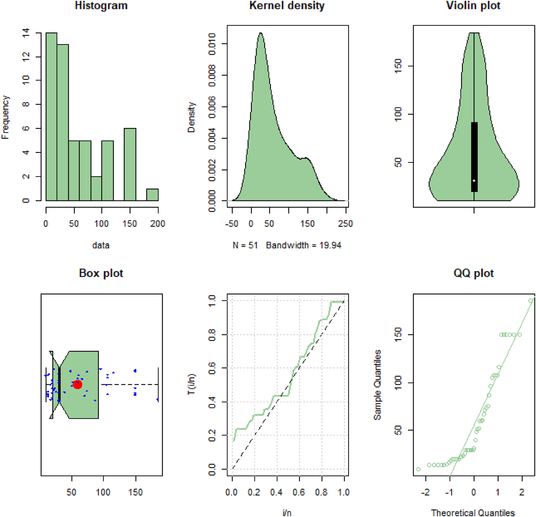
Plots for liver cancer data.

Figure (6.a):

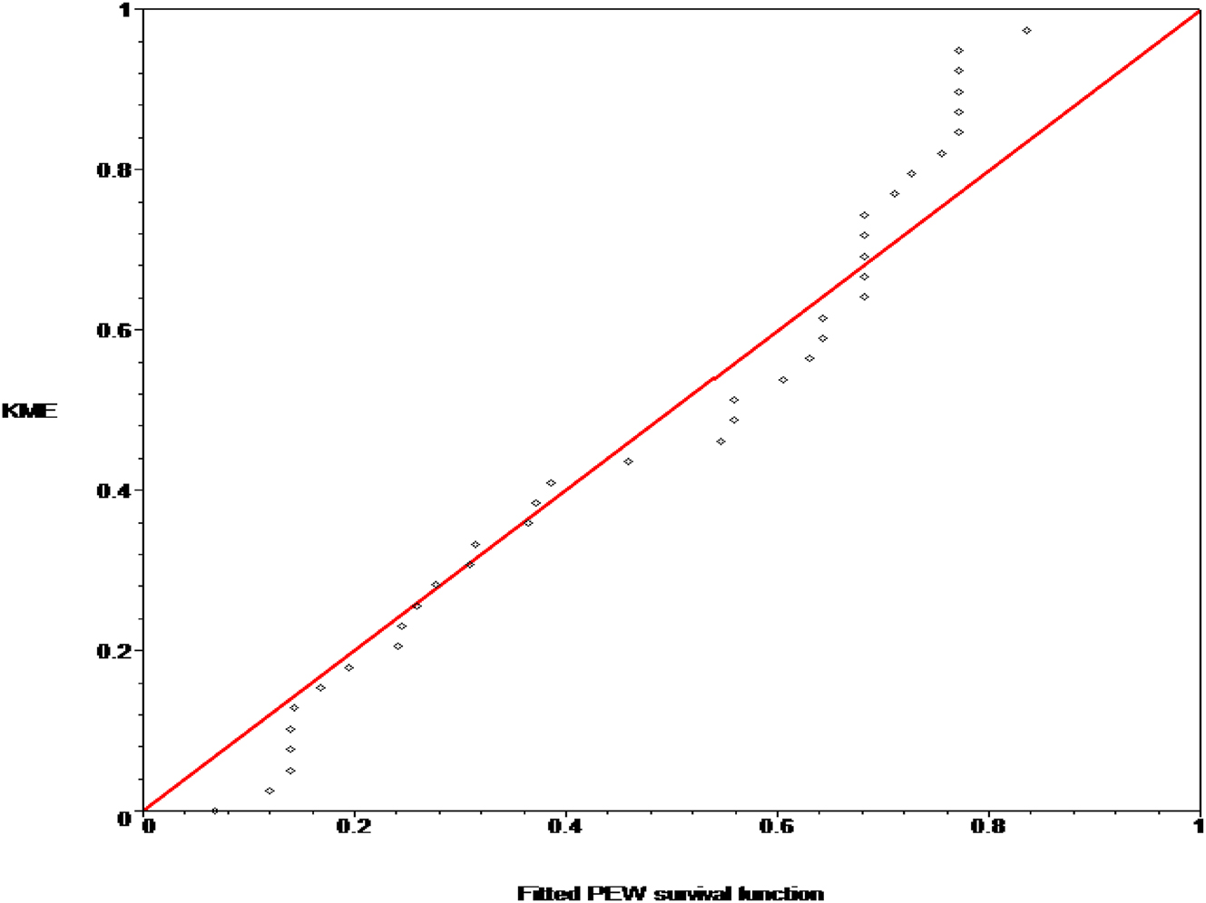
KME versus the fitted PE-W survival function in a p-p point plot.

Figure (6.b):

KME versus the fitted MOEW and Weibull survival functions in a p-p plot.

Table 2:

An analysis examining the censored data’s MLEs, ln, model selection for PE-W, Marshal-Olkin extend Weibull (MOEW) and Weibull models.

	Estimates			Statistics
Models	γ	θ	λ	ln	AIC	BIC	CAIC
PE-W	1.1021	1.2663	0.00557	−208.211	−214.211	−214.109	−214.722
MOEW	0.6033	9.8791	0.0759	−210.469	−216.469	−216.367	−216.980
Weibull	0.0805		71.605	−311.172	−315.172	−315.104	−315.422

For the Liver Cancer data, we observe that the PE-W model’s AIC, BIC, and CAIC are greater than those of the comparable MOEW and Weibull distributions, indicating that the PE-W model fits the data more closely. Furthermore, the parameters γ, θ and λ have the approximate 95 % two-sided confidence intervals [1.070, 1.134], [0.7031, 1.828] and [0.001, 0.185], respectively.

The likelihood ratio test (LRT) is used to assess the null hypothesis H ₀ (the data follow the Weibull distribution). A = −2[ ln t i , γ , λ - ln t i , γ , θ , λ ] is a likelihood ratio statistic that has roughly a chi-square distribution with two degrees of freedom under H ₀. With regard to the liver cancer data, we employed the likelihood ratio test (LRT) statistic to evaluate the hypothesis H ₀: the data follow the Weibull distribution versus H ₁: the data follow the PEW distribution.

under H 1 thus x L 1 = 2 − 208.211 − − 311.172 = 205.922 > χ 1.0 . 05 2 = 3.84 .

Consequently, the null hypothesis cannot be accepted; that is, the LRT rejects the notion that the Weibull model is appropriate.

Assume that δ ₁, δ ₂, …, δ _n are the censoring indicators and t ₁, t ₂, …, t _n are the ordered survival periods. The product-limit estimator, sometimes referred to as the Kaplan-Meier estimator (KME) (Kaplan and Meier [36]), is:

G ̄ n t = ∏ t : t i ≤ t i = 1 , … , n 1 − δ ( i ) n − i + 1 , t > 0 .

The fitted PE-W survival function’s points are visually quite close to the 45o line, suggesting a very good fit when compared to the fitted MOEW and Weibull survival functions.

Figure 7 displays the calculated hazard rate function for PE-W distribution

Figure 7:

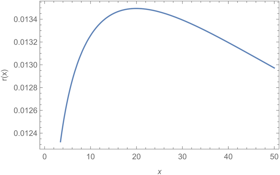
Based on the liver cancer data, the estimated HRF of PE-W(α, β, θ) distribution.

Example 2: Lung cancer data

Lagakos & Williams [37] and Lee & Wolfe [38] collected the data, this reflects the 61 lung cancer patients receiving cyclophosphamide treatment (in weeks) (see Figure 8 and Table 3).

33 uncensored observations:

0.43, 2.86, 3.14, 3.14, 3.43, 3.43, 3.71, 3.86, 6.14, 6.86, 9.00, 9.43, 10.71, 10.86, 11.14, 13.00, 14.43, 15.71, 18.43, 18.57, 20.71, 29.14, 29.71, 40.57, 48.57, 49.43, 53.86, 61.86, 66.57, 68.71, 68.96, 72.86, 72.86
28 censored observations:

0.14, 0.14, 0.29, 0.43, 0.57, 0.57, 1.86, 3.00, 3.00, 3.29, 3.29, 6.00, 6.00, 6.14, 8.71, 10.57, 11.86, 15.57, 16.57, 17.29, 18.71, 21.29, 23.86, 26.00, 27.57, 32.14, 33.14, 47.29.

Figure 8:

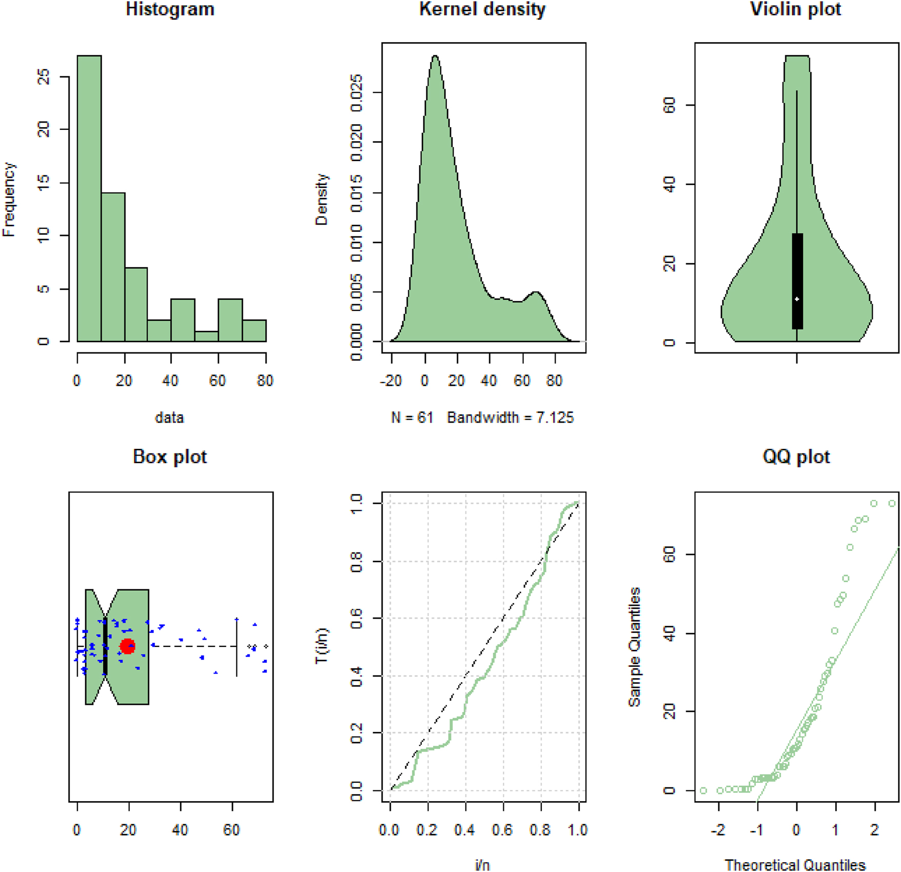
Plots for lung cancer data.

Figure (8.a):

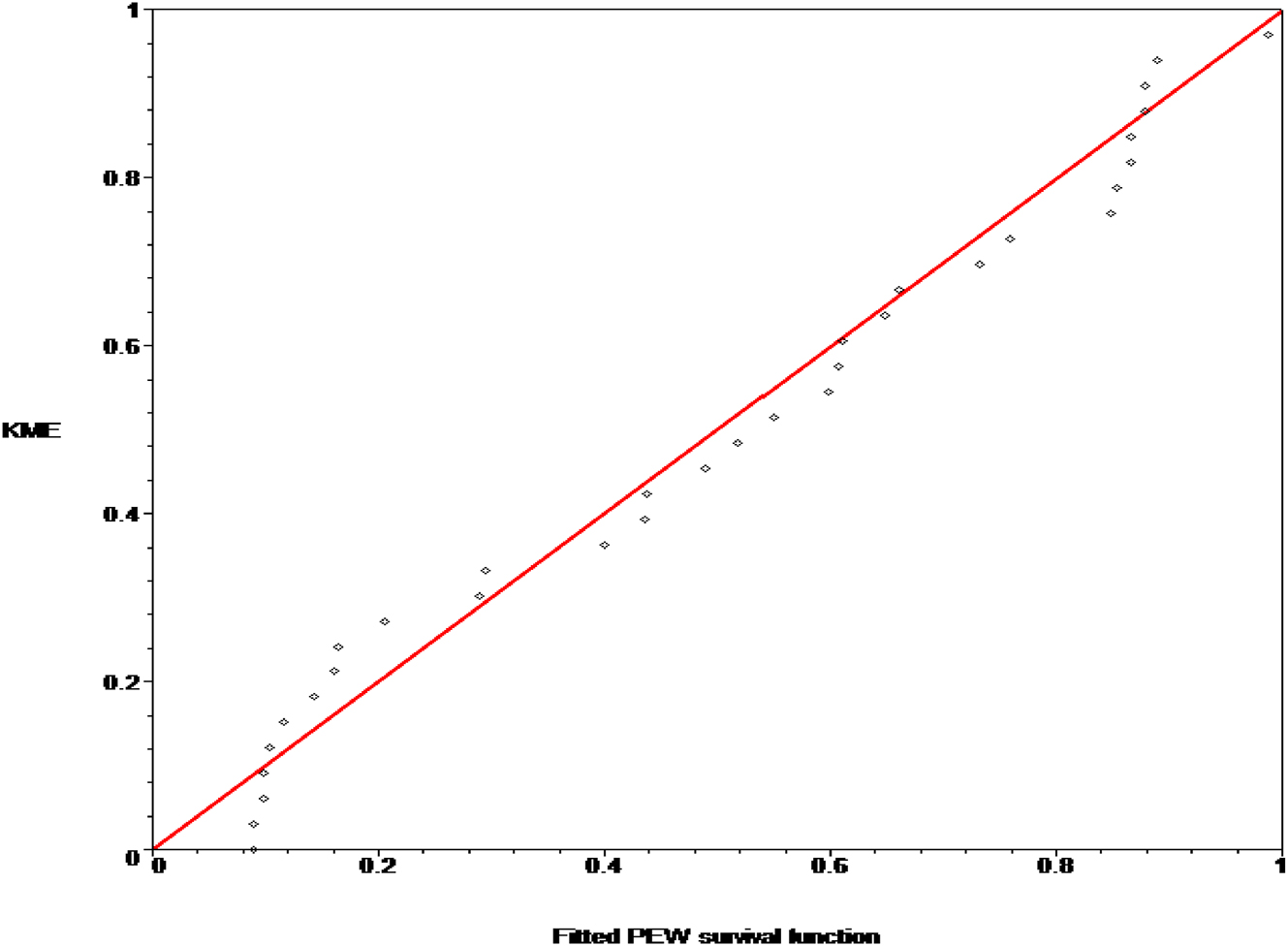
KME against the fitted PE-W survival function in a p-p plot.

Figure (8.b):

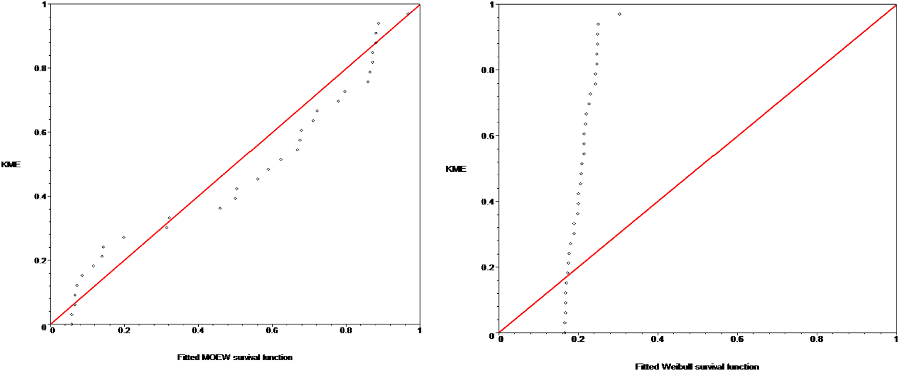
KME against the fitted MOEW and Weibull survival functions in a p-p plot.

Table 3:

An analysis examining the censored data’s MLEs and Statistics for PE-W, MOEW and Weibull distributions.

	Estimates			Statistics
Models	γ	θ	λ	ln	AIC	BIC	CAIC
PE-W	1.145	1.595	0.01177	−147.91	−153.91	−154.08	−154.33
MOEW	0.4762	20.2657	0.3807	−149.34	−155.343	−155.59	−155.764
Weibull	0.6573		0.0845	−152.93	−156.91	−157.04	−157.14

For the Lung Cancer Data, comparing the AIC, BIC, and CAIC of the equivalent MOEW and Weibull distributions, we find that the PE-W model has higher values., indicating that the PE-W model fits the data more closely. Furthermore, the parameters γ, θ and λ have approximate 95 % two-sided confidence intervals [0.847, 1.443], [0.0109, 1.097] and [0.0009, 0.0225], respectively.

Further, using the likelihood ratio test (LRT) statistic, we assess the following hypotheses: H ₀: the data are Weibull distributed; and H ₁: the data are PE-W distributed. Under H ₁ thus X _L1 = 2[−147.91 − (−149.34)] = 10.039 > χ 1.0 . 05 2 = 3.84 , consequently, the null hypothesis cannot be accepted; that is, the Weibull model’s applicability is rejected by the LRT.

Assume that the ordered survival periods are t ₁, t ₂, …, t _n and the related censoring indicators are δ ₁, δ ₂, …, δ _n. The KME is:

G ̄ n t = ∏ t : t i ≤ t i = 1 , … , n 1 − δ ( i ) n − i + 1 , t > 0 .

The fitted PE-W survival function’s points are visually quite close to the 45o line, suggesting a very good fit when compared to the fitted MOEW and Weibull survival functions.

Figure 9 displays the calculated hazard rate function for the PE-W distributions.

Figure 9:

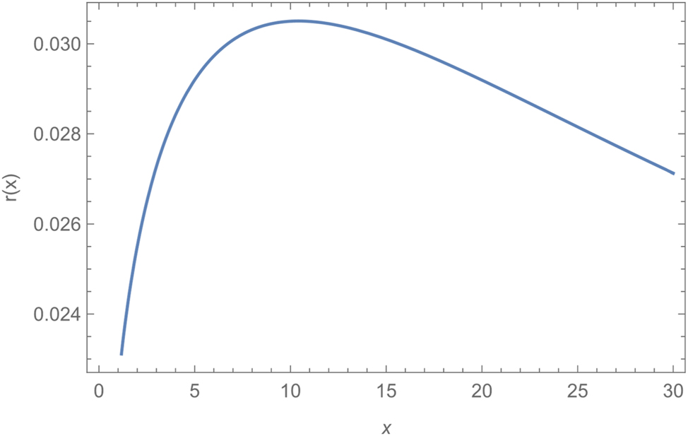
The HRF estimate of PE-W(γ, θ, λ) distribution based on the lung cancer data.

7.2 Complete data

Example 3: Glass fibers data

We will study a complete data set by Smith and Naylor [39], It involves 63 observations that show the glass fibers’ strength (see Figure 10 and Table 4).

Figure 10:

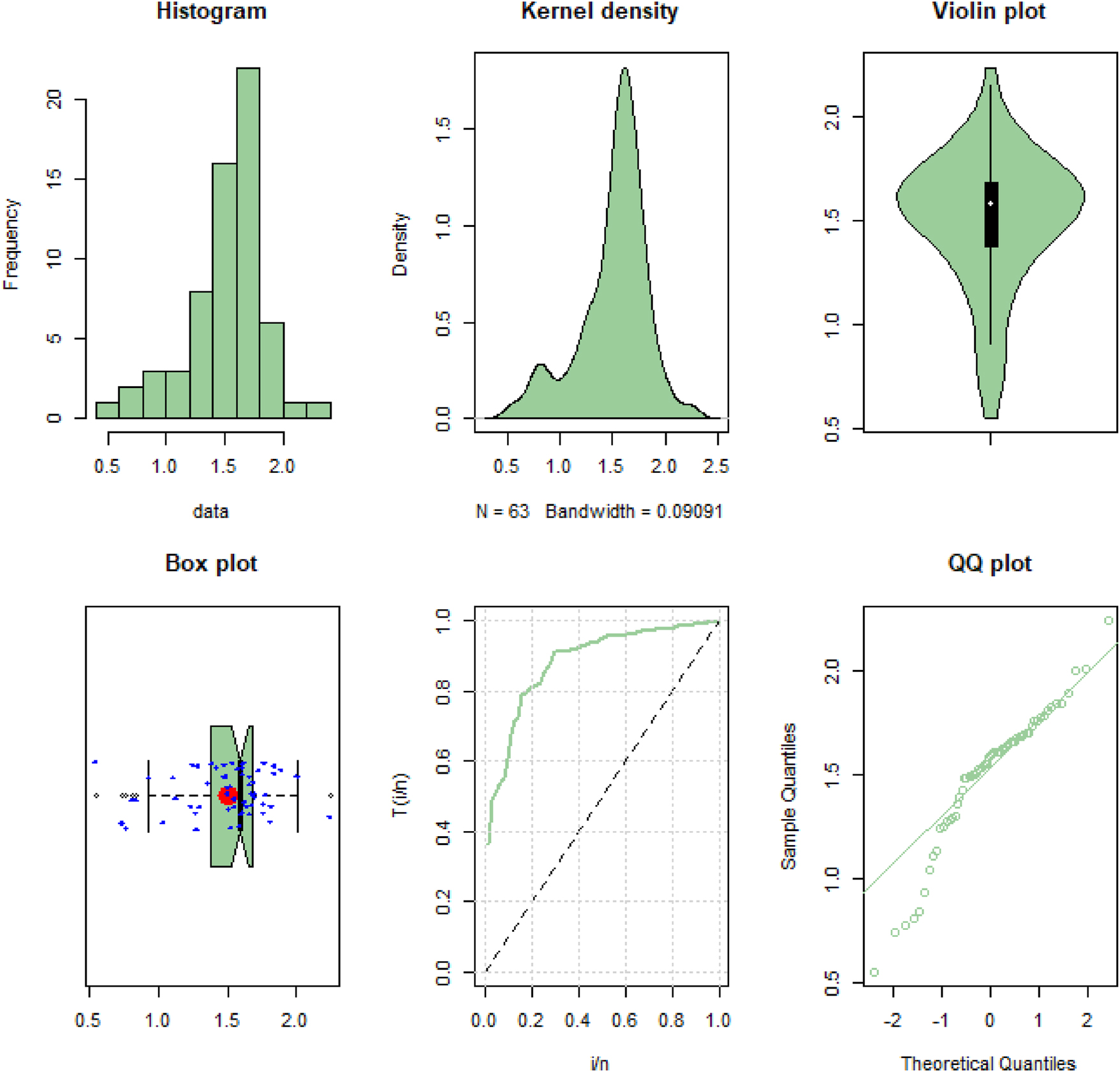
Plots for glass fibers data.

Table 4:

An analysis examining the censored data’s MLEs and statistics for PE-W, MOEW and Weibull distributions.

	Estimates			Statistics
Models	γ	θ	λ	ln	AIC	BIC	CAIC
PE-W	0.0588	68.508	5.7942	−15.239	−21.239	−21.453	−21.646
MOEW	7.3402	0.0068	0.3326	−22.815	−28.815	−29.029	−29.221
Weibull	13.152		0.0006	−73.547	−77.546	−77.690	−77.747

0.55, 0.74, 0.77, 0.81, 0.84, 0.93, 1.04, 1.11, 1.13, 1.24, 1.25, 1.27, 1.28, 1.29, 1.30, 1.36, 1.39, 1.42, 1.48, 1.48, 1.49, 1.49, 1.50, 1.50, 1. 51, 1.52, 1.53, 1.54, 1.55, 1.55, 1.58, 1.59, 1.60, 1.61, 1.61, 1.61, 1.61, 1.62, 1.62, 1.63, 1.64, 1.66, 1.66, 1.66, 1.67, 1.68, 1.68, 1.69, 1.70, 1.70, 1.73, 1.76, 1.76, 1.77, 1.78, 1.81, 1.82, 1.84 1.84, 1.89, 2.00, 2.01, 2.24

For the glass fibers data, the corresponding MOEW and Weibull distributions’ AIC, BIC, and CAIC are fewer than those of the PE-W model, which indicates that the PE-W model fits the data more closely. Furthermore, the parameters γ, θ and λ have the approximate 95 % two-sided confidence intervals [5.672, 5.917], [66.69, 70.33] and [0.0001, 0.2577], respectively.

Using the likelihood ratio test (LRT) statistic, we evaluated each hypothesis by comparing the data to the Weibull distribution (H ₀) and the PE-W distribution (H ₁).

With regard to the liver cancer data, using the likelihood ratio test (LRT) statistic, we evaluated each hypothesis by comparing the data to the Weibull distribution (H ₀) and the PE-W distribution (H ₁). Under H ₁ thus X _L1 = 2 − 15.238 − − 73.547 = 116.618 > χ 1.0 . 05 2 = 3.84 , consequently, the null hypothesis cannot be accepted; that is, the Weibull model is not acceptable, according to the LRT.

Figure 11 displays the calculated hazard rate function for the PE-W distribution.

Figure 11:

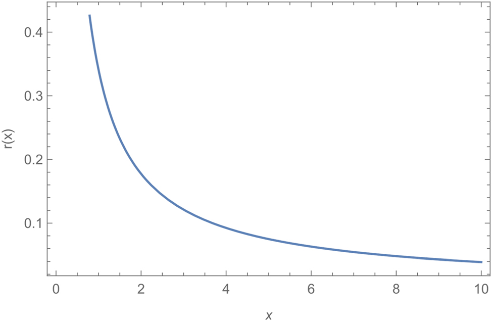
The HRF estimate of PE-W(γ, θ, λ) distribution based on the glass fibers data.

8 Conclusions

In this paper, a new family is proposed for adding one parameter to a continuous distribution by using countable mixture of PE distribution. The added parameters provide additional flexibility for fitting diverse shapes of data. Some of the properties of the new family are derived. A detailed study is provided for the particular case when the extended distribution is the Weibull distribution. The derived properties include: PDF, its shape, HRF, moments, and MLE. We note that for PE-W distribution, the model selections BIC, AIC and CAIC are higher than the corresponding BIC, AIC and CAIC of the MOEW, and Weibull distributions. Also, the fitted PE-W survival function indicates strong linear relationship between the empirical and fitted survival functions compared with the fitted MOEW and Weibull survival functions. All these results lead us to select the PE-W distribution as the best distribution for the given data.

Corresponding author: Yusra A. Tashkandy, Department of Statistics and Operations Research, College of Science, King Saud University, P.O. Box 2455, Riyadh 11451, Saudi Arabia, E-mail: ytashkandy@ksu.edu.sa

Funding source: Ongoing Research Funding program (ORF-2025-488) King Saud University, Riyadh, Saudi Arabia.

Award Identifier / Grant number: (ORF-2025-488).

Acknowledgments

This study was supported by Ongoing Research Funding program (ORF-2025-488) King Saud University, Riyadh, Saudi Arabia. The work was also funded by the University of Jeddah, Jeddah, Saudi Arabia, under grant No. (UJ-23-DR-263). The authors extend their sincere gratitude to both King Saud University and the University of Jeddah for their financial and technical support.

Funding information: This research was supported by the Ongoing Research Funding program at King Saud University, Riyadh, Saudi Arabia (ORF-2025-488). The work was also funded by the University of Jeddah, Jeddah, Saudi Arabia, under grant No. (UJ-23-DR-263). The authors extend their sincere gratitude to both King Saud University and the University of Jeddah for their financial and technical support.
Author contribution: All authors have accepted responsibility for the entire content of this manuscript and approved its submission.
Conflict of interest: The authors state no conflict of interest.
Data availability statement: The datasets generated and/or analysed during the current study are available from the corresponding author on reasonable request.

References

1. Marshall, AN, Olkin, I. A new method for adding a parameter to a family of distributions with applications to the exponential and Weibull families. Biometrika 1997;84:641–52.10.1093/biomet/84.3.641Search in Google Scholar

2. AL-Hussaini, EK, Gharib, M. A new family of distributions as a countable mixture with Poisson added parameter. J Stat Theor Appl 2009;8:169–90.Search in Google Scholar

3. AL-Hussaini, EK, Ghitany, ME. On certain countable mixtures of absolutely continuous distributions. Metron LXIII 2005:30–53.Search in Google Scholar

4. Alzaatreh, A, Lee, C, Famoye, F. A new method for generating families of continuous distributions. Metron 2013;71:63–79. https://doi.org/10.1007/s40300-013-0007-y.Search in Google Scholar

5. Ghitany, ME, Al-Hussaini, EK, AlJarallah, RA. Marshall–Olkin extended Weibull distribution and its application to censored data. J Appl Stat 2005;32:1025–34. https://doi.org/10.1080/02664760500165008.Search in Google Scholar

6. Cordeiro, GM, de Castro, M. A new family of generalized distributions. J Stat Comput Simulat 2011;81:883–98. https://doi.org/10.1080/00949650903530745.Search in Google Scholar

7. Bourguignon, M, Silva, RB, Cordeiro, GM. The Weibull-G family of probability distributions. J Data Sci 2014;12:53–68. https://doi.org/10.6339/jds.201401_12(1).0004.Search in Google Scholar

8. Brito, E, Cordeiro, GM, Yousof, HM, Alizadeh, M, Silva, GO. The ToppLeone odd log-logistic family of distributions. J Stat Comput Simulat 2017;87:3040–58. https://doi.org/10.1080/00949655.2017.1351972.Search in Google Scholar

9. Gharib, M, Mohammed, BI, Al-Ajmi, AH. A new method for adding two parameters to a family of distributions with application. J Stat Appl Pro 2017;6:1–11. https://doi.org/10.18576/jsap/060305.Search in Google Scholar

10. Chipepa, F, Oluyede, B, Makubate, B, Fagbamigbe, AF. The beta odd Lindley-G family of distributions with applications. J Probab Stat Sci 2019;17:51–83.Search in Google Scholar

11. Alsadat, N, Nagarjuna, VB, Hassan, AS, Elgarhy, M, Ahmad, H, Almetwally, EM. Marshall–Olkin Weibull–Burr XII distribution with application to physics data. AIP Adv 2023;13:095325. https://doi.org/10.1063/5.0172143.Search in Google Scholar

12. Dina, AR, Yusra, AT, BakrBalogun, MEOS, Hasaballah, MM. Analysis of Marshall–Olkin extended Gumbel type-II distribution under progressive type-II censoring with applications. AIP Adv 2024;14:37–55.10.1063/5.0210905Search in Google Scholar

13. Ahmed, MG, Yusra, AT, Bakr, ME, Anoop, K, Moyazzem, HM, Ehab, MA. Fitting COVID-19 datasets to a new statistical model. AIP Adv 2024;14:085110. https://doi.org/10.1063/5.0214473.Search in Google Scholar

14. Aljohani, HM. The single and double inverse Pareto–Burr XII distribution: properties, estimation methods, and real-life data applications. AIP Adv 2024;14:055217. https://doi.org/10.1063/5.0203919.Search in Google Scholar

15. Mahmoudi, E, Zakerzadeh, H. Generalized Poisson–Lindley distribution. Commun Stat – Theor Methods 2010;39:1785–98. https://doi.org/10.1080/03610920902898514.Search in Google Scholar

16. Bereta, EM, Louzada, F, Franco, MA. The Poisson-Weibull distribution. Adv Appl Stat 2011;22:107–18.Search in Google Scholar

17. Bhati, D, Kumawat, P, Gómez-Déniz, E. A new count model generated from mixed Poisson transmuted exponential family with an application to health care data. Commun Stat – Theor Methods 2017;46:11060–76.10.1080/03610926.2016.1257712Search in Google Scholar

18. Miao, Y, Kook, JH, Lu, Y, Guindani, M, Vannucci, M. Scalable Bayesian variable selection regression models for count data. In: Flexible Bayesian regression modelling. Cambridge, MA, USA: Academic Press; 2020:187–219 pp.10.1016/B978-0-12-815862-3.00015-9Search in Google Scholar

19. Altun, E. A new generalization of geometric distribution with properties and applications. Commun Stat – Simulat Comput 2020;49:793–807. https://doi.org/10.1080/03610918.2019.1639739.Search in Google Scholar

20. Altun, E, Cordeiro, GM, Ristic, MM. A one-parameter compounding discrete distribution. J Appl Stat 2022;49:1935–56.10.1080/02664763.2021.1884846Search in Google Scholar PubMed PubMed Central

21. Fazal, A, Bashir, S. Family of Poisson distribution and its application. Int J Appl Math Stat Sci (IJAMSS) 2017;6:1–18.Search in Google Scholar

22. Estela, MP, Bereta, FL, Maria, AD. The Poisson-Weibull distribution. Adv Appl Stat 2011;22:107–18.Search in Google Scholar

23. Ana, P, Betsabé, B, Gauss, MC. The beta Weibull Poisson distribution. Chil J Stat 2013;4:3–26.Search in Google Scholar

24. Cordeiro, GM, Lemonte, AJ. On the marshall-olkin extended weibull distribution. Stat Pap 2013;54:333–53. https://doi.org/10.1007/s00362-012-0431-8.Search in Google Scholar

25. Muhammad, B, Muhammad, M, Muhammad, A. Weibull-exponential distribution and its application in monitoring industrial process. Math Probl Eng 2021;6650237:1–13.10.1155/2021/9960264Search in Google Scholar

26. Kumaraswamy, K, Bhatra Charyulu, NC. Compound distribution of Poisson-Weibull. Int J Math Stat Invent (IJMSI) 2021;9:29–34.Search in Google Scholar

27. Adam, BS, Mastor, ON, Joseph, MU, Nada, MA, Ahmed, Z. The extended exponential weibull distribution: properties, inference, and applications to real-life data. Complexity 2022;2022:1–13.10.1155/2022/4068842Search in Google Scholar

28. Fisher, RA. The mathematical theory of probabilities and its applications to frequency curves and statistical models. New York: Macmillan; 1936.Search in Google Scholar

29. Teicher, H. On the mixture of distributions. Ann Math Stat 1960;31:55–73. https://doi.org/10.1214/aoms/1177705987.Search in Google Scholar

30. Kenney, JF, Keeping, ES. Mathematics of statistics, 3rd ed., Part 1. London: Chapman & Hall Ltd; 1962.Search in Google Scholar

31. Moors, JA. A quantile alternative for kurtosis. J R Stat Soc Ser D (The Statistician) 1988;37:25–32. https://doi.org/10.2307/2348376.Search in Google Scholar

32. Schwarz, G. Estimating the dimension of a model. Ann Stat 1978;6:461–4. https://doi.org/10.1214/aos/1176344136.Search in Google Scholar

33. Akaike, H. Fitting autoregressive models for prediction. Ann Inst Stat Math 1969;21:243–7. https://doi.org/10.1007/bf02532251.Search in Google Scholar

34. Bozdogan, H. Model selection and Akaike’s information criterion (AIC): the general theory and its analytical extensions. Psychometrika 1987;52:345–70. https://doi.org/10.1007/bf02294361.Search in Google Scholar

35. Attia, AF, Mahmoud, MA, Abdul-Moniem, IB. On testing for exponential better than used in average class of life distributions based on the U-test. In: The proceeding of the 39 th annual conference on statistics. SR Cairo University-Egypt; 2004:11–14 pp.Search in Google Scholar

36. Kaplan, EL, Meier, P. Nonparametric estimation from incomplete observations. J Am Stat Assoc 1958;53:457–81. https://doi.org/10.1080/01621459.1958.10501452.Search in Google Scholar

37. Lagakos, SW, Williams, JS. Models for censored survival analysis: a cone class of variable-sum models. Biometrika 1978;65:181–9. https://doi.org/10.1093/biomet/65.1.181.Search in Google Scholar

38. Lee, S, Wolfe, RA. A simple test for independent censoring under the proportional hazards model. Biometrics 1998;54:1176–82. https://doi.org/10.2307/2533867.Search in Google Scholar

39. Smith, RL, Naylor, JC. A comparison of maximum likelihood and Bayesian estimators for the three-parameter weibull distribution. J R Stat Soc Ser C (Applied Statistics) 1987;36:358–69. https://doi.org/10.2307/2347795.Search in Google Scholar

Received: 2025-03-13

Accepted: 2025-11-09

Published Online: 2025-12-04

This work is licensed under the Creative Commons Attribution 4.0 International License.

Articles in the same Issue

https://doi.org/10.1515/phys-2025-0241

Keywords for this article

Poisson exponential; Poisson exponential Weibull model; mean inactivity time; censored and complete data; model selections; p-p plot

Creative Commons

BY 4.0