Studying bifurcations and chaotic dynamics in the generalized hyperelastic-rod wave equation through Hamiltonian mechanics

Hongwei Ma; Ziming Liu; Yiqun Sun; Peng Guo; Jianming Qi

doi:10.1515/phys-2025-0183

Article Open Access

Studying bifurcations and chaotic dynamics in the generalized hyperelastic-rod wave equation through Hamiltonian mechanics

Hongwei Ma , Ziming Liu , Yiqun Sun , Peng Guo and Jianming Qi

Published/Copyright: August 7, 2025

Published by

Become an author with De Gruyter Brill

Submit Manuscript Author Information Explore this Subject

From the journal Open Physics Volume 23 Issue 1

Abstract

This article introduces a novel modified G ′ G 2 expansion method, combined with Maple software, for solving the exact solutions of the generalized hyperelastic-rod wave equation (GHRWE). The GHRWE has extensive applications in various fields, including the study of dark soliton molecules in nonlinear optics, the propagation of longitudinal waves in fractional derivative viscoelastic materials, and the investigation of the local well-posedness and dispersive limit behavior of the generalized hyperelastic rod wave equation. Through this method, we have obtained a variety of solutions, including U-shaped dark solitons, inverted U-shaped solitons, single W-shaped solitons, and bright-dark alternating solitons. These solutions not only enrich the solution set of GHRWE but also provide a theoretical basis for understanding and predicting behaviors in nonlinear dynamical systems. Our research delves into the impact of fractional order variations on soliton solution characteristics, such as shape and amplitude, and analyzes the effects of different fractional derivative selections on soliton properties. In addition, a significant contribution of this study is the construction of the Hamiltonian system for GHRWE using the trial equation method, revealing complex bifurcations and chaotic dynamics that have eluded previous research. Ultimately, we employed the Chebyshev method, renowned for its exceptional accuracy and numerical stability, to rigorously validate our analytical solutions, ensuring minimal error margins. Through these efforts, we have not only advanced the understanding of GHRWE but also provided new perspectives and tools for research in related fields.

Keywords: fractional order derivative; solitons; Hamiltonian; bifurcations; chaotic dynamics

1 Introduction

Nonlinear partial differential equations (NPDEs) constitute a vital mathematical apparatus for encapsulating a broad array of physical phenomena. In the realm of physics, they capture the essence of processes such as heat conduction within solid materials and the mechanics of wave transmission. In the biological sciences, NPDEs are indispensable for modeling complex systems. Their utility extends to various other disciplines, including electrical engineering, quantum mechanics, plasma physics, and the study of fluid dynamics. During the past three decades, there has been a surge in the development and application of fractional NPDEs, which incorporate noninteger order derivatives in either time or space. This advancement has generated considerable academic and practical interest, resulting in a proliferation of scholarly gatherings and in-depth research endeavors. Fractional NPDEs have proven to be particularly useful in a multitude of sectors, including engineering, physics, biology, fluid dynamics, and financial markets, among several others. Their versatility and adaptability make them a cornerstone in the mathematical modeling of complex systems across these diverse fields [1–8].

Finding analytical solutions for nonlinear PDEs, especially precise solitary wave solutions, poses a challenging task. Various mathematical techniques are employed to derive explicit solitary wave solutions. These include the direct algebraic method [9], the sine-Gordon expansion method [10], Hirota’s direct method [11], the innovative MEDA method [12,13], the Riccati equation mapping method [14], the Sardar subequation method [15], and applications involving Jacobi elliptic functions [16]. These methods represent diverse approaches aimed at extracting exact solutions from nonlinear PDEs, each offering unique advantages depending on the specific characteristics of the equation under study.

The background model of the generalized hyperelastic-rod wave equation (GHRWE) can be traced back to the study of elastic compressible materials, which is widely applied in the field of elasticity mechanics and holds significant research value. This model describes the nonlinear dynamic behavior of a one-dimensional hyperelastic rod under large deformations and is one of the classic models in the field of nonlinear dynamics. The GHRWE model was proposed to capture and describe the complex dynamic response of fluids or rod-like structures when subjected to external forces, especially in situations involving large deformations and nonlinear factors. The GHEWE finds extensive applications in characterizing the wave behavior of fibers, rods, and various hyperelastic materials. It’s instrumental in analyzing the vibration response of flexible components, such as satellite deployable arms and antennas, during different phases like launch, orbit, and operation. This analysis aids in optimizing designs for better structural performance and stability. As a mathematical framework for describing the dynamics of intricate materials and structures, the GHEWE carries substantial research and practical value in numerous fields. In this study, we delve deeper into the nonlinear, conformable time-fractional dynamics inherent to the GHRWE. Integrals and fractional derivatives play a vital role in modeling materials and processes with nonlinear temporal behaviors, such as anomalous diffusion marked by variable memory effects. Cohen developed geometric finite difference schemes specifically designed for the GHEWE [17]. Meanwhile, Tian approached the GHRWE by integrating Kato’s theory, conservation laws, and blow-up rates [18]. Va employed the Hirota bilinear method to manipulate rogue waves in compressible hyperelastic plates [19]. Demiray derived exact solitary wave solutions for both the Kraenkel-Manna-Merle system and the GHRWE using the generalized Kudryashov method [20]. Novruzov investigated the blow-up phenomenon associated with the GHRWE [21].

Research on chaos, fractals, and soliton theory in nonlinear differential equations has emerged as a prominent area of focus in the contemporary scientific research. Houwe et al. conducted an analysis of modulation instability, bifurcation phenomena, and solitonic waves within the nonlinear Schrödinger equation (NLSE) [22]. Akinyemi’s team explored solitary waves and modulation instability within higher-order NLSE contexts [23]. Mathanaranjan’s group made significant advancements in understanding chirped optical solitons and their stability [24]. Akinyemi also investigated optical soliton solutions for a nonlinear Schrödinger equation characterized by parabolic nonlinearity [25]. Debin et al. identified soliton wave solutions for the (2+1)-dimensional Sawada-Kotera equation [26]. Wazwaz and Kaur derived optical solitons using both the variational iteration method [27] and an enhanced ( G ′ G ) expansion method [28] and they utilized various ansatz methods to generate dark-bright solitons [29] and analyzed these solitons using Hirota’s simplified approach [30]. Raut et al. identified exact solutions through discrimination system methods [31] and explored integrability, breathers, lumps, and quasi-periodic structures via the Hirota transformation [32–34]. Roy’s team explored bilinear Bäcklund transformations, Lax pairs, breather and lump waves, as well as soliton interactions [35]. Meanwhile, Sarkar’s group employed the ( G ′ G ) method to investigate acoustic shocks, solitary waves, and periodic structures [36]. Mahdy et al. scrutinized the stability, existence, and uniqueness of solutions for fractional order partial differential equations (PDEs) [37].

Fractional-order derivatives are frequently preferred over traditional derivatives because they offer a continuous spectrum of solutions within the range (0, 1], as opposed to the distinct, separate solutions provided by classical derivatives. The team led by Morales-Delgado employed fractional conformable derivatives of the Liouville-Caputo variety [38], while Solís Pérez’s work implemented these derivatives in the context of the Liouville-Caputo sense [39]. Yépez-Martínez and his associates studied nonlinear differential equations utilizing conformable derivatives [40]. Consequently, conformable fractional order derivatives have gained widespread acceptance and application in various research fields [12,41,42].

In this study, fractional-order GHRWE attracts more attention compared to integer-order GHRWE due to its superior adaptability, model accuracy, dynamic response of complex materials, and broad application prospects. In 2023, Simbanefayi’s team investigated the integer-order GHRWE to seek travelling wave solutions [43]. In 2024, Shahzad’s group studied the exact solutions of fractional-order GHRWE [44]. GHRWE is essentially a nonlinear partial differential equation, and from the outcomes of these previous articles [43,44], aspects such as chaos, fractals, sensitivity analysis, and comparisons of solutions under different fractional derivative forms have not yet been investigated. In this article, we will employ the trial equation method to construct the Hamiltonian structure of GHRWE and investigate the associated behaviors such as chaos and fractals. Furthermore, we focus on a specific technique: the improved G ′ G 2 -expansion method. This method yields a diverse range of solutions, including periodic, singular, dark soliton, and peakon wave solutions. The innovation of this work lies in obtaining diverse soliton solutions for fractional-order GHRWE and exploring chaos, fractals, and sensitivity analysis, aspects not covered in the previous literature [42–44]. We anticipate these solutions to find applications in materials science and engineering, structural dynamics, biomedical applications, and aerospace engineering.

In this article, we define the conformable fractional derivative (CFD) of a function f : [ 0 , ∞ ) → R of order β as follows:

D z β ( f ) ( z ) = lim ε → 0 f ( z + ε z 1 − β ) − f ( z ) ε , z > 0 , β ∈ ( 0 , 1 ] .

If the aforementioned limit exists, then f is considered β -differentiable. Let β be in the interval (0, 1], and assume that both f and g are β -differentiable at a point z > 0 . Under these conditions, D β adheres to the following properties:

(1) ( 1 ) D β ( a f + b g ) = a D β ( f ) + b D β ( g ) , for all a , b ∈ R ( 2 ) D β ( z n ) = n z n − β , for all n ∈ R ( 3 ) D z β ( f ( g ( z ) ) ) = z 1 − β g ′ ( z ) f ′ ( g ( z ) ) .

The properties mentioned in [40] are applied for CFD. The fractional-order GHRWE studied in this article is primarily analyzed in the context of CFD.

2 Mathematical formulation

2.1 Application trial equation method to GHRWE

In this subsection, we employ the trial equation method to construct the Hamiltonian structure of GHRWE, laying the groundwork for obtaining exact solutions of the equations and exploring chaos, fractals, and related phenomena.

(2) ϕ t − ϕ x x t − α ϕ x x + λ ϕ x + g ( ϕ ) x = 0 ,

where g ( ϕ ) is a C 2 -smooth nonlinear function and ϕ ( x , t ) represents the fluid velocity along the horizontal x -axis. In addition, α and λ denote a nonnegative constant and any real constant, respectively. (Eq. (2) is derived from Eq. (1.1) in Reference [43] and Eq. (4) in Reference [44].) The GHRWE is a mathematical model used to describe wave propagation through thin, hyperelastic structures such as fibers or rods. This equation accounts for the nonlinear and dispersive properties of the material. By utilizing the GHRWE, scientists and engineers can more accurately understand and predict wave behavior in hyperelastic materials, leading to improved designs and applications across various industries. This equation provides a more realistic representation of the physical phenomena associated with wave propagation in these materials. The mathematical form of the GHRWE model can describe the variation of fluid velocity along the horizontal x -axis, which includes nonlinear terms, enabling the model to simulate more complex physical phenomena, such as wave propagation and stability issues in fluid dynamics. In addition, the GHRWE model also involves in-depth research on wave phenomena in fluid dynamics, especially in exploring chaos, fractals, and related phenomena. The proposal and study of this model not only enrich the research content of nonlinear dynamics and fluid mechanics in theory but also provide a powerful analytical tool in practical applications such as pipeline flow, hydropower generation, and ocean engineering. Through the study of the GHRWE model, scientists and engineers can better understand and predict wave phenomena in fluids, thereby playing an important role in engineering design and disaster prevention. We obtain a general form of the GHRWE by substituting g ( ϕ ) x = θ ϕ ϕ x + ρ ϕ x x x in Eq. (2).

(3) ϕ t − ϕ x x t + α ϕ x x + 2 τ ϕ ϕ x + 3 θ ϕ 2 ϕ x − λ ϕ x ϕ x x − ϕ ϕ x x x = 0 ,

where τ , θ , and α , are the parameters. Eq. (3) represents significant physical models in mathematical physics. By applying the CFD, we obtain the following form:

(4) ∂ t β ϕ − ∂ t β ( ∂ x x ) ϕ + α ∂ x x ϕ + 2 τ ϕ ∂ x ϕ + 3 θ ϕ 2 ∂ x ϕ − λ ∂ x ϕ ∂ x x ϕ − ϕ ∂ x x x ϕ = 0 ,

where β denotes the fractional operator with 0 < β ≤ 1 in Eq. (3). The exact solitary wave solutions for Eq. (4) are found by applying a wave transformation to convert the partial differential equation (PDE) into an ordinary differential equation (ODE). This transformation is given by ϕ ( x , t ) = Ψ ( ξ ) , where ξ = a x − b t β β , where a represents the amplitude of the wave, b is the speed of the wave, and Ψ ( ξ ) is a real-valued function. By applying this wave transformation, we convert Eq. (4) into the following ODE form:

(5) ( b a 2 − a 3 Ψ ) Ψ ″ + 1 2 ( a 3 − λ ) ( Ψ ′ ) 2 + ( − b + α a ) Ψ + a τ Ψ 2 + a θ Ψ 3 = 0 ,

where Ψ is a polynomial and Ψ ′ = d d ξ .

Next, we employ the trial equation method to construct the solution for Eq. (5). We assume that the solution to Eq. (5) satisfies the trial equations as described in [45,46]:

(6) Ψ ″ = ∑ i = 0 m r i Ψ i , Ψ ′ 2 = p 0 + ∑ i = 0 m 2 r i i + 1 Ψ i + 1 ,

where p 0 and r i , i = 0 , 1 , 2 , 3 , … are constants that need to be determined later. According to Eq. (6), we apply the balance principle to Eq. (5) so that Ψ Ψ ″ has the same degree as Ψ 3 . This implies m + 1 = 3 , thus m = 2 . Therefore, we obtain:

(7) Ψ ″ = r 0 + r 1 Ψ + r 2 Ψ 2 ;

(8) ( Ψ ′ ) 2 = p 0 + 2 r 0 Ψ + r 1 Ψ 2 + 2 r 2 3 Ψ 3 .

Taking Eqs. (7) and (8) into Eq. (5) and setting the coefficients of Ψ ( ξ ) to zero, we utilize the symbolic computation software Maple to obtain the following results:

(9) p 0 = A + B λ 4 + 2 a 3 λ 3 − a 6 λ 2 − 2 a 9 λ , r 2 = 3 a θ 2 a 3 + λ , r 1 = ( λ 2 − a 3 λ ) p 0 2 b 2 a 4 + b − α a b a 2 , r 0 = ( λ − a 3 ) p 0 2 b a 2 ,

where A = 12 a 7 b 3 θ + 8 a 8 b 2 τ + 4 a 9 b α − 4 a 8 b 2 , B = ( 6 a 6 b α − 6 a 5 b 2 + 4 a 5 b 2 τ ) λ + ( 2 a 3 b α − 2 a 2 b 2 ) λ 2 .

2.2 The modified G ′ G 2 -expansion method

Below, we introduce the modified G ′ G 2 -expansion method [47,48], which, like the generalized Riccati equation mapping method and ( G ′ G ) -expansion method [5,49,50], is a trial equation method. This means it uses solutions of known equations to explore the exact solutions of unknown nonlinear equations. We have chosen the modified G ′ G 2 -expansion method because it is simple and easy to understand, capable of discovering a large number of solutions, especially some new solutions that have not been identified in the relevant literature before. The method applied in this article is based on the same principles as those in references [51,52], but it is more complex in form than [51] and simpler than [52].

First, let’s consider the following nonlinear fractional PDE:

(10) P ( U , U x β , U t β , U x x 2 β , U x t 2 β … ) = 0 , 0 < β ≤ 1 ,

in this context, P is a polynomial consisting of the unknown function U ( x , t ) and its fractional derivative. Next, the recently developed modified G ′ G 2 -expansion approach is then described in detail.

Step 1. Taking H : U ( x , t ) = U ( ξ ) , where ξ = a x − b t β β , into Eq. (10), and improving Eq. (10) into the next-order integer differential equation:

(11) T ( U , U ′ , U ″ , U ‴ , … ) = 0 ,

in Eq. (11), a polynomial of U ( ξ ) and its derivatives is called T .

Step 2. We propose that the solution to Eq. (11) can be expressed as a polynomial in terms of G ′ G 2 :

(12) U ( ξ ) = α 0 + ∑ z = 1 i ( α i G ′ G 2 i + β i G ′ G 2 − i ) ,

in Eq. (12), the function G = G ( ξ ) fulfills the following differential equation:

(13) G ′ G 2 ′ = σ + μ G ′ G 2 + ρ G ′ G 2 2 .

In this context, σ , μ , and ρ are arbitrary constants. The positive integer m can be found by using the homogeneous balance between the nonlinear variables in Eq. (11) and the highest order derivatives.

Step 3. By substituting Eq. (12) into Eq. (11) and utilizing (13), Eq. (11) is transformed into a polynomial in terms of G ′ G 2 . By setting the coefficients of each polynomial term to zero, a set of algebraic equations for α m , … , ρ , μ is obtained.

Step 4. The specific values of the constants α m , … , α 0 , β 1 , … , β m can be determined from the system of algebraic equations derived in Step 3. Given that Eq. (13) has five possible solutions, the exact solutions of the given Eq. (10) can thus be obtained.

(14) Case 1: If μ = 0 , σ ρ > 0 , then G ′ G 2 ( ξ ) = σ ρ σ C 1 cos σ ρ ξ + C 2 sin σ ρ ξ C 2 cos σ ρ ξ − C 1 sin σ ρ ξ ; Case 2: If σ ρ < 0 , μ = 0 , then G ′ G 2 ( ξ ) = ∣ σ ρ ∣ − σ C 1 sinh 2 ∣ σ ρ ∣ ξ + C 2 cosh 2 ∣ σ ρ ∣ ξ + C 2 C 1 cosh 2 ∣ σ ρ ∣ ξ + C 1 sinh 2 ∣ σ ρ ∣ ξ − C 2 ; Case 3: If σ = 0 , ρ ≠ 0 , μ = 0 , then G ′ G 2 ( ξ ) = − C 1 ρ ( C 1 ξ + C 2 ) ; Case 4: If μ ≠ 0 , Δ ≥ 0 , then G ′ G 2 ( ξ ) = − μ 2 ρ − Δ ( C 1 cosh Δ 2 ξ + C 2 sinh Δ 2 ξ ) 2 ρ ( C 2 cosh Δ 2 ξ + C 1 sinh Δ 2 ξ ) ; Case 5: If μ ≠ 0 , Δ < 0 , then G ′ G 2 ( ξ ) = − μ 2 ρ − − Δ ( C 1 cos − Δ 2 ξ − C 2 sin − Δ 2 ξ ) 2 ρ ( C 2 cos − Δ 2 ξ + C 1 sin − Δ 2 ξ ) ,

where A ( ξ ) = G ′ G 2 ( ξ ) , C 1 , C 2 are free constants, and Δ = μ 2 − 4 ρ σ .

Step 5. By applying the inverse transform T − 1 to the solution u ( ξ ) , where ξ = a x − b t β β , the exact solutions of the original fractional nonlinear PDE can be obtained.

2.3 Employing the modified G ′ G 2 -expansion method to the Eq. (7)

Since we applied the trial equation method to simplify Eq. (5), following earlier calculations, we obtained a new simplified nonlinear Eq. (7). Therefore, here, we directly solve Eq. (7), and the exact solutions obtained are actually solutions of Eq. (5).

In accordance with the principles of the ( G ′ ⁄ G 2 ) -expansion method, we propose that the exact solution of Eq. (7) can be expressed as follows:

(15) U ( ξ ) = a 0 + ∑ n = 1 m ( a n G ′ G 2 n + b n G ′ G 2 − n ) .

By applying the principle of homogeneous equilibrium, we can easily determine that m = 2 . Therefore, we can formulate the general solution of Eq. (7) as follows:

(16) U ( ξ ) = a 0 + a 1 G ′ G 2 + a 2 G ′ G 2 2 + b 1 G ′ G 2 − 1 + b 2 G ′ G 2 − 2 ,

where, a 0 , a 1 , a 2 , b 1 , and b 2 are the unknown constants.

We gather all terms with the same power of G ′ G 2 and use Eqs. (7) and (16). By applying Eq. (13) and setting the indeterminate coefficients of the same G ′ G 2 functions to zero, we derive the equations.

(17) 6 a 2 ρ 2 − r 2 a 2 2 = 0 , 2 a 1 ρ 2 + 10 a 2 μ ρ − 2 r 2 a 1 a 2 = 0 , 3 a 1 μ ρ + 4 a 2 μ 2 + 8 a 2 σ ρ − 2 r 2 a 0 a 2 − r 2 a 1 2 − r 1 a 2 = 0 , a 1 μ 2 + 2 a 1 σ ρ + 6 a 2 μ σ − 2 r 2 a 0 a 1 − 2 r 2 b 1 a 2 − r 1 a 1 = 0 , a 1 μ σ + 2 a 2 σ 2 + b 1 μ ρ + 2 b 2 ρ 2 − r 2 a 0 2 − 2 r 2 a 1 b 1 − 2 r 2 a 2 b 2 − r 1 a 0 − r 0 = 0 , b 1 μ 2 + 2 b 1 σ ρ + 6 b 2 μ ρ − 2 r 2 a 0 b 1 − 2 r 2 a 1 b 2 − r 1 b 1 = 0 , 3 b 1 σ μ + 4 b 2 μ 2 + 8 b 2 ρ σ − 2 r 2 a 0 b 2 − r 2 a 1 2 − r 1 b 2 = 0 , 2 b 1 σ 2 + 10 b 2 μ σ − 2 r 2 b 1 b 2 = 0 , 6 b 2 σ 2 − r 2 b 2 2 = 0 .

The equations given by Eq. (17) are solved using Maple 2021, resulting in 15 different sets for the undetermined coefficients:

(18) Set1. a 0 = μ 2 + 8 ρ σ − r 1 2 r 2 , a 1 = 0 , b 1 = 6 σ μ r 2 , a 2 = 0 , b 2 = 6 σ 2 r 2 , U 1 ( x , t ) = μ 2 + 8 ρ σ − r 1 2 r 2 + 6 σ μ r 2 ρ σ C 1 cos σ ρ a x − b t β β + C 2 sin σ ρ a x − b t β β C 2 cos σ ρ a x − b t β β − C 1 sin σ ρ a x − b t β β − 1

+ 6 σ 2 r 2 ρ σ C 1 cos σ ρ a x − b t β β + C 2 sin σ ρ a x − b t β β C 2 cos σ ρ a x − b t β β − C 1 sin σ ρ a x − b t β β − 2 , where , r 2 ≠ 0 , μ = 0 , ( 4 ρ σ ) 2 − r 1 2 + 4 r 0 r 2 = 0 , and σ ρ > 0 .

(19) Set2. a 0 = μ 2 + 8 ρ σ − r 1 2 r 2 , a 1 = 0 , b 1 = 6 σ μ r 2 , a 2 = 0 , b 2 = 6 σ 2 r 2 , U 2 ( x , t ) = μ 2 + 8 ρ σ − r 1 2 r 2 + 6 σ μ r 2 − ∣ σ ρ ∣ σ C 1 sinh 2 ∣ σ ρ ∣ a x − b t β β + C 2 cosh 2 ∣ σ ρ ∣ a x − b t β β + C 2 C 1 cosh 2 ∣ σ ρ ∣ a x − b t β β + C 1 sinh 2 ∣ σ ρ ∣ a x − b t β β − C 2 − 1 + 6 σ 2 r 2 − ∣ σ ρ ∣ σ C 1 sinh 2 ∣ σ ρ ∣ a x − b t β β + C 2 cosh 2 ∣ σ ρ ∣ a x − b t β β + C 2 C 1 cosh 2 ∣ σ ρ ∣ a x − b t β β + C 1 sinh 2 ∣ σ ρ ∣ a x − b t β β − C 2 − 2 , where , σ ρ < 0 , μ = 0 , ( 4 ρ σ ) 2 − r 1 2 + 4 r 0 r 2 = 0 , and r 2 ≠ 0 .

(20) Set3. a 0 = μ 2 + 8 ρ σ − r 1 2 r 2 , a 1 = 0 , b 1 = 6 σ μ r 2 , a 2 = 0 , b 2 = 6 σ 2 r 2 , U 3 ( x , t ) = μ 2 + 8 ρ σ − r 1 2 r 2 + 6 σ μ r 2 − C 1 ρ C 1 a x − b t β β + C 2 − 1 + 6 σ 2 r 2 − C 1 ρ C 1 a x − b t β β + C 2 − 2 , where , σ = 0 , ρ ≠ 0 , μ = 0 , ( 4 ρ σ ) 2 − r 1 2 + 4 r 0 r 2 = 0 , and r 2 ≠ 0 .

(21) Set4. a 0 = μ 2 + 8 ρ σ − r 1 2 r 2 , a 1 = 0 , b 1 = 6 σ μ r 2 , a 2 = 0 , b 2 = 6 σ 2 r 2 , U 4 ( x , t ) = μ 2 + 8 ρ σ − r 1 2 r 2 + 6 σ μ r 2 − μ 2 ρ − Δ C 1 cosh Δ 2 a x − b t β β + C 2 sinh Δ 2 a x − b t β β 2 ρ C 2 cosh Δ 2 a x − b t β β + C 1 sinh Δ 2 a x − b t β β − 1

+ 6 σ 2 r 2 − μ 2 ρ − Δ C 1 cosh Δ 2 a x − b t β β + C 2 sinh Δ 2 a x − b t β β 2 ρ C 2 cosh Δ 2 a x − b t β β + C 1 sinh Δ 2 a x − b t β β − 2 , where , Δ ≥ 0 , μ ≠ 0 , ( μ 2 − 4 ρ σ ) 2 − r 1 2 + 4 r 0 r 2 = 0 , and r 2 ≠ 0 .

(22) Set5. a 0 = μ 2 + 8 ρ σ − r 1 2 r 2 , a 1 = 0 , b 1 = 6 σ μ r 2 , a 2 = 0 , b 2 = 6 σ 2 r 2 , U 5 ( x , t ) = μ 2 + 8 ρ σ − r 1 2 r 2 + 6 σ μ r 2 − μ 2 ρ − − Δ C 1 cos − Δ 2 a x − b t β β − C 2 sin − Δ 2 a x − b t β β 2 ρ C 2 cos − Δ 2 a x − b t β β + C 1 sin − Δ 2 a x − b t β β − 1

+ 6 σ 2 r 2 − μ 2 ρ − − Δ C 1 cos − Δ 2 a x − b t β β − C 2 sin − Δ 2 a x − b t β β 2 ρ C 2 cos − Δ 2 a x − b t β β + C 1 sin − Δ 2 a x − b t β β − 2 , where , μ ≠ 0 , Δ < 0 , ( μ 2 − 4 ρ σ ) 2 − r 1 2 + 4 r 0 r 2 = 0 , and r 2 ≠ 0 .

(23) Set6. a 0 = μ 2 + 8 ρ σ − r 1 2 r 2 , a 1 = 6 ρ μ r 2 , b 1 = 0 , a 2 = 6 ρ 2 r 2 , b 2 = 0 , U 6 ( x , t ) = μ 2 + 8 ρ σ − r 1 2 r 2 + 6 ρ μ r 2 ρ σ C 1 cos σ ρ a x − b t β β + C 2 sin σ ρ a x − b t β β C 2 cos σ ρ a x − b t β β − C 1 sin σ ρ a x − b t β β

+ 6 ρ 2 r 2 ( ρ σ [ C 1 cos ( σ ρ a x − b t β β ) + C 2 sin σ ρ a x − b t β β C 2 cos σ ρ a x − b t β β − C 1 sin σ ρ a x − b t β β ] ) 2 , where , r 2 ≠ 0 , μ = 0 , ( 4 ρ σ ) 2 − r 1 2 + 4 r 0 r 2 = 0 , and σ ρ > 0 .

(24) Set7. a 0 = μ 2 + 8 ρ σ − r 1 2 r 2 , a 1 = 6 ρ μ r 2 , b 1 = 0 , a 2 = 6 ρ 2 r 2 , b 2 = 0 , U 7 ( x , t ) = μ 2 + 8 ρ σ − r 1 2 r 2 + 6 σ μ r 2 − ∣ σ ρ ∣ σ C 1 cos ∣ σ ρ ∣ a x − b t β β + C 2 sin ∣ σ ρ ∣ a x − b t β β C 2 cos ∣ σ ρ ∣ a x − b t β β − C 1 sin ∣ σ ρ ∣ a x − b t β β

+ 6 ρ 2 r 2 − ∣ σ ρ ∣ σ C 1 sinh 2 ∣ σ ρ ∣ a x − b t β β + C 2 cosh 2 ∣ σ ρ ∣ a x − b t β β + C 2 C 1 cosh 2 ∣ σ ρ ∣ a x − b t β β + C 1 sinh 2 ∣ σ ρ ∣ a x − b t β β − C 2 2 , where , σ ρ < 0 , μ = 0 , ( 4 ρ σ ) 2 − r 1 2 + 4 r 0 r 2 = 0 , and r 2 ≠ 0 .

(25) Set8. a 0 = μ 2 + 8 ρ σ − r 1 2 r 2 , a 1 = 6 ρ μ r 2 , b 1 = 0 , a 2 = 6 ρ 2 r 2 , b 2 = 0 , U 8 ( x , t ) = μ 2 + 8 ρ σ − r 1 2 r 2 + 6 ρ μ r 2 − C 1 ρ C 1 a x − b t β β + C 2 + 6 ρ 2 r 2 − C 1 ρ C 1 a x − b t β β + C 2 2 , where , σ = 0 , ρ ≠ 0 , μ = 0 , ( 4 ρ σ ) 2 − r 1 2 + 4 r 0 r 2 = 0 , and r 2 ≠ 0 .

(26) Set9. a 0 = μ 2 + 8 ρ σ − r 1 2 r 2 , a 1 = 6 ρ μ r 2 , b 1 = 0 , a 2 = 6 ρ 2 r 2 , b 2 = 0 , U 9 ( x , t ) = μ 2 + 8 ρ σ − r 1 2 r 2 + 6 ρ μ r 2 − μ 2 ρ − Δ C 1 cosh Δ 2 a x − b t β β + C 2 sinh Δ 2 a x − b t β β 2 ρ ( C 2 cosh Δ 2 a x − b t β β + C 1 sinh Δ 2 a x − b t β β )

+ 6 ρ 2 r 2 − μ 2 ρ − Δ C 1 cosh Δ 2 a x − b t β β + C 2 sinh Δ 2 a x − b t β β 2 ρ C 2 cosh Δ 2 a x − b t β β + C 1 sinh Δ 2 a x − b t β β 2 , where , μ ≠ 0 , Δ ≥ 0 , ( μ 2 − 4 ρ σ ) 2 − r 1 2 + 4 r 0 r 2 = 0 , and r 2 ≠ 0 .

(27) Set10. a 0 = μ 2 + 8 ρ σ − r 1 2 r 2 , a 1 = 6 ρ μ r 2 , b 1 = 0 , a 2 = 6 ρ 2 r 2 , b 2 = 0 , U 10 ( x , t ) = μ 2 + 8 ρ σ − r 1 2 r 2 + 6 ρ μ r 2 − μ 2 ρ − − Δ C 1 cos − Δ 2 a x − b t β β − C 2 sin − Δ 2 a x − b t β β 2 ρ C 2 cos − Δ 2 a x − b t β β + C 1 sin − Δ 2 a x − b t β β

+ 6 ρ 2 r 2 − μ 2 ρ − − Δ C 1 cos − Δ 2 a x − b t β β − C 2 sin − Δ 2 a x − b t β β 2 ρ C 2 cos − Δ 2 a x − b t β β + C 1 sin − Δ 2 a x − b t β β 2 , where , μ ≠ 0 , Δ < 0 , ( μ 2 − 4 ρ σ ) 2 − r 1 2 + 4 r 0 r 2 = 0 , and r 2 ≠ 0 .

(28) Set 11. a 0 = μ 2 + 8 ρ σ − r 1 2 r 2 , a 1 = 6 ρ μ r 2 , b 1 = 6 σ μ r 2 , a 2 = 6 ρ 2 r 2 , b 2 = 6 σ 2 r 2 s , U 11 ( x , t ) = μ 2 + 8 ρ σ − r 1 2 r 2 + 6 ρ μ r 2 ρ σ C 1 cos σ ρ a x − b t β β + C 2 sin σ ρ a x − b t β β C 2 cos σ ρ a x − b t β β − C 1 sin σ ρ a x − b t β β

+ 6 ρ 2 r 2 ρ σ C 1 cos σ ρ a x − b t β β + C 2 sin σ ρ a x − b t β β C 2 cos σ ρ a x − b t β β − C 1 sin σ ρ a x − b t β β 2 + 6 σ μ r 2 ρ σ C 1 cos σ ρ a x − b t β β + C 2 sin σ ρ a x − b t β β C 2 cos σ ρ a x − b t β β − C 1 sin σ ρ a x − b t β β − 1

+ 6 σ 2 r 2 ρ σ C 1 cos σ ρ a x − b t β β + C 2 sin σ ρ a x − b t β β C 2 cos σ ρ a x − b t β β − C 1 sin σ ρ a x − b t β β − 2 , where , σ ρ > 0 , μ = 0 , 256 ρ 2 σ 2 − r 1 2 + 4 r 2 r 0 = 0 , and r 2 ≠ 0 .

(29) Set 12. a 0 = μ 2 + 8 ρ σ − r 1 2 r 2 , a 1 = 6 ρ μ r 2 , b 1 = 6 σ μ r 2 , a 2 = 6 ρ 2 r 2 , b 2 = 6 σ 2 r 2 , U 12 ( x , t ) = μ 2 + 8 ρ σ − r 1 2 r 2 + 6 ρ μ r 2 − ∣ σ ρ ∣ σ C 1 sinh 2 ∣ σ ρ ∣ a x − b t β β + C 2 cosh 2 ∣ σ ρ ∣ a x − b t β β + C 2 C 1 cosh 2 ∣ σ ρ ∣ a x − b t β β + C 1 sinh 2 ∣ σ ρ ∣ a x − b t β β − C 2

+ 6 ρ 2 r 2 − ∣ σ ρ ∣ σ C 1 sinh 2 ∣ σ ρ ∣ a x − b t β β + C 2 cosh 2 ∣ σ ρ ∣ a x − b t β β + C 2 C 1 cosh 2 ∣ σ ρ ∣ a x − b t β β + C 1 sinh 2 ∣ σ ρ ∣ a x − b t β β − C 2 2 + 6 σ μ r 2 − ∣ σ ρ ∣ σ C 1 sinh 2 ∣ σ ρ ∣ a x − b t β β + C 2 cosh 2 ∣ σ ρ ∣ a x − b t β β + C 2 C 1 cosh 2 ∣ σ ρ ∣ a x − b t β β + C 1 sinh 2 ∣ σ ρ ∣ a x − b t β β − C 2 − 1 + 6 σ 2 r 2 − ∣ σ ρ ∣ σ C 1 sinh 2 ∣ σ ρ ∣ a x − b t β β + C 2 cosh 2 ∣ σ ρ ∣ a x − b t β β + C 2 C 1 cosh 2 ∣ σ ρ ∣ a x − b t β β + C 1 sinh 2 ∣ σ ρ ∣ a x − b t β β − C 2 − 2 , where , σ ρ < 0 , μ = 0,256 ρ 2 σ 2 − r 1 2 + 4 r 2 r 0 = 0 , and r 2 ≠ 0 .

(30) Set13. a 0 = μ 2 + 8 ρ σ − r 1 2 r 2 , a 1 = 6 ρ μ r 2 , b 1 = 6 σ μ r 2 , a 2 = 6 ρ 2 r 2 , b 2 = 6 σ 2 r 2 , U 13 ( x , t ) = μ 2 + 8 ρ σ − r 1 2 r 2 + 6 ρ μ r 2 − C 1 ρ C 1 a x − b t β β + C 2 + 6 ρ 2 r 2 − C 1 ρ C 1 a x − b t β β + C 2 2 . + 6 σ μ r 2 − C 1 ρ C 1 a x − b t β β + C 2 − 1 + 6 σ 2 r 2 − C 1 ρ C 1 a x − b t β β + C 2 − 2 , where , σ = 0 , ρ ≠ 0 , μ = 0,256 ρ 2 σ 2 − r 1 2 + 4 r 2 r 0 = 0 , and r 2 ≠ 0 .

(31) Set14. a 0 = μ 2 + 8 ρ σ − r 1 2 r 2 , a 1 = 6 ρ μ r 2 , b 1 = 6 σ μ r 2 , a 2 = 6 ρ 2 r 2 , b 2 = 6 σ 2 r 2 , U 14 ( x , t ) = μ 2 + 8 ρ σ − r 1 2 r 2 + 6 ρ μ r 2 − μ 2 ρ − Δ ( C 1 cosh Δ 2 a x − b t β β + C 2 sinh Δ 2 a x − b t β β ) 2 ρ ( C 2 cosh Δ 2 a x − b t β β + C 1 sinh Δ 2 a x − b t β β ) + 6 ρ 2 r 2 − μ 2 ρ − Δ C 1 cosh Δ 2 a x − b t β β + C 2 sinh Δ 2 a x − b t β β 2 ρ C 2 cosh Δ 2 a x − b t β β + C 1 sinh Δ 2 a x − b t β β 2 .

+ 6 σ μ r 2 − μ 2 ρ − Δ C 1 cosh Δ 2 a x − b t β β + C 2 sinh Δ 2 a x − b t β β 2 ρ C 2 cosh Δ 2 a x − b t β β + C 1 sinh Δ 2 a x − b t β β − 1 + 6 σ 2 r 2 − μ 2 ρ − Δ C 1 cosh Δ 2 a x − b t β β + C 2 sinh Δ 2 a x − b t β β 2 ρ C 2 cosh Δ 2 a x − b t β β + C 1 sinh Δ 2 a x − b t β β − 2 , where , μ ≠ 0 , Δ ≥ 0 , 288 μ + 8 ρ 9 ρ σ 2 + 256 μ μ + 9 ρ 8 ρ σ + μ 4 − r 1 2 + 4 r 2 r 0 = 0 , and r 2 ≠ 0 .

(32) Set15. a 0 = μ 2 + 8 ρ σ − r 1 2 r 2 , a 1 = 6 ρ μ r 2 , b 1 = 6 σ μ r 2 , a 2 = 6 ρ 2 r 2 , b 2 = 6 σ 2 r 2 , U 15 ( x , t ) = μ 2 + 8 ρ σ − r 1 2 r 2 + 6 ρ μ r 2 − μ 2 ρ − − Δ C 1 cos − Δ 2 a x − b t β β − C 2 sin − Δ 2 a x − b t β β 2 ρ C 2 cos − Δ 2 a x − b t β β + C 1 sin − Δ 2 a x − b t β β + 6 ρ 2 r 2 − μ 2 ρ − − Δ ( C 1 cos − Δ 2 a x − b t β β − C 2 sin − Δ 2 a x − b t β β ) 2 ρ C 2 cos − Δ 2 a x − b t β β + C 1 sin − Δ 2 a x − b t β β 2

+ 6 σ μ r 2 − μ 2 ρ − − Δ C 1 cos − Δ 2 − C 2 sin − Δ 2 a x − b t β β 2 ρ C 2 cos − Δ 2 a x − b t β β + C 1 sin − Δ 2 a x − b t β β − 1 + 6 σ 2 r 2 − μ 2 ρ − − Δ C 1 cos − Δ 2 a x − b t β β − C 2 sin − Δ 2 a x − b t β β 2 ρ C 2 cos − Δ 2 a x − b t β β + C 1 sin − Δ 2 a x − b t β β − 2 , where , μ ≠ 0 , Δ < 0 , 288 μ + 8 ρ 9 ρ σ 2 + 256 μ μ + 9 ρ 8 ρ σ + μ 4 − r 1 2 + 4 r 2 r 0 = 0 , and r 2 ≠ 0 .

3 Findings and discussion

3.1 Visual interpretation of the derived solutions

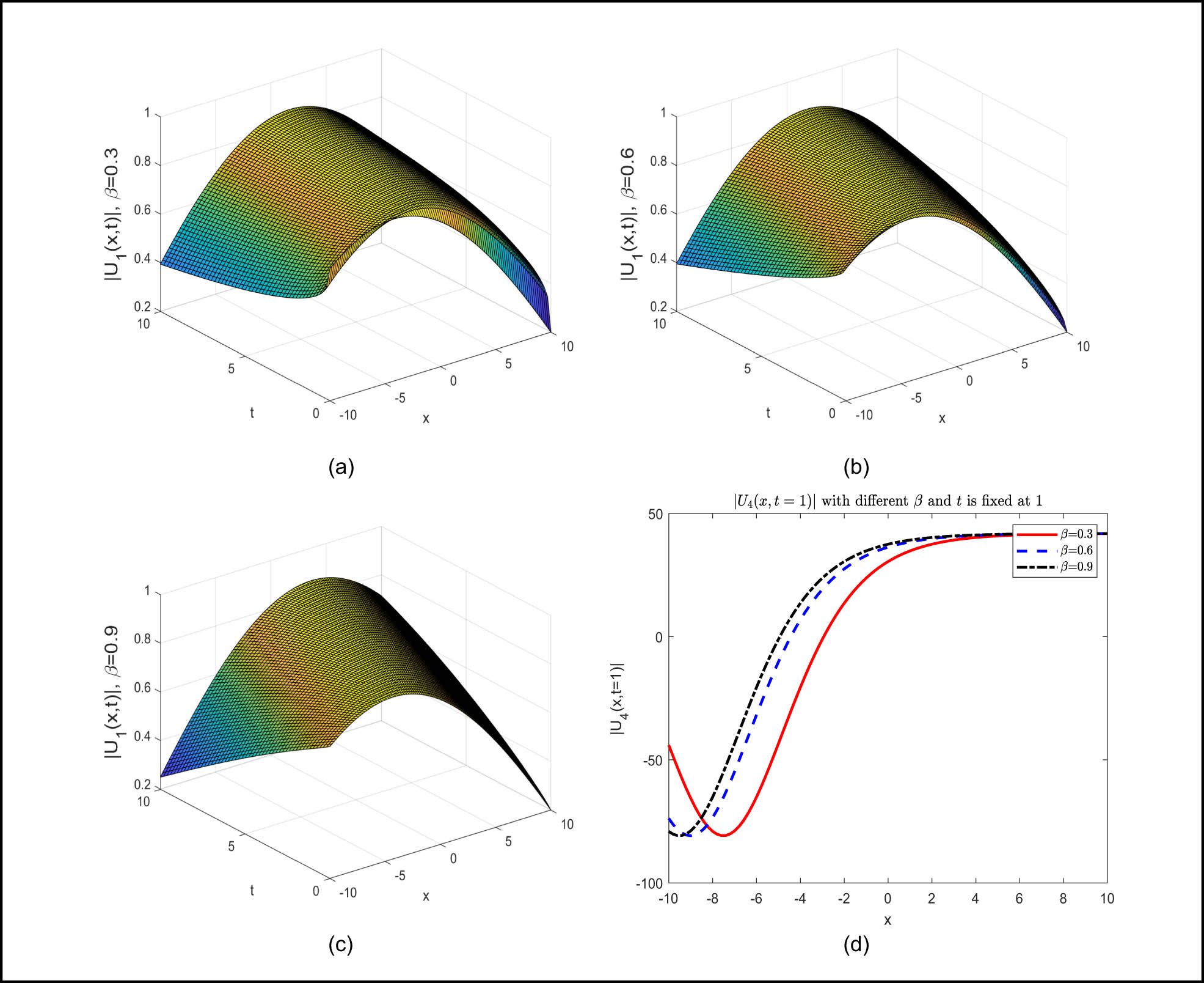
In this section, we delve into the graphical analysis of the solitary wave structures that have been extracted for a range of constant values. In this context, soliton solutions represent a distinct category of solutions that are localized, are stable, and maintain their shape and amplitude as they propagate. Solitons are important in various fields, including physics, engineering, and applied mathematics. Based on the ideas of [53], moreover, we explored the influence of changes in different values of the fractional-order β on the shape and propagation of solitons.

Figure 1: The 3D representations of the individual parabolic solitons, denoted by ∣ U 1 ( x , t ; β ) ∣ , are illustrated in Figure 1(a)–(c). In the 2D cross-sectional diagram in Figure 1(d), it is clearly observed that as the fraction β increases, there is a little change in the shape. It can be concluded that the variation in fraction β have minimal impact on the soliton. We set the added independent factors as follows: α = 1.1 , τ = − 1.5 , λ = 0.5 , C 1 = − 10 , C 2 = 0 , θ = 0.5 , a = 1 , b = 0.09 , ρ = 1 , and μ = 0 . The change in the value of β alters the waveform, reflecting the influence of parameters in the GHRWE model on the wave characteristics of the hyperelastic rod, such as the wave shape and propagation properties. This helps in a deeper understanding of the complex dynamic responses of the hyperelastic rod under actual loading scenarios, providing an intuitive visual basis for the applied research of GHRWE in the field of elastomechanics.

$Figure 1 Individual U-shaped solitons in 3D representation: The CFD results for ∣ U 1 ( x , t ; β ) ∣ | {U}_{1}\left(x,t;\hspace{0.33em}\beta )| are depicted through three-dimensional plots for different β \beta . In addition, (d) shows the 2D waveforms of (a)–(c) after a diffusion time of t t = 5 s. The following parameters were adjusted: α = 1.1 \alpha =1.1 , τ = − 1.5 \tau =-1.5 , λ = 0.5 \lambda =0.5 , C 1 = − 10 {C}_{1}=-10 , C 2 = 0 {C}_{2}=0 , θ = 0.5 \theta =0.5 , a = 0.2 a=0.2 , b = 0.09 b=0.09 , σ = 1 \sigma =1 , and μ = 0 \mu =0 . The change in the value of β \beta alters the waveform, reflecting the influence of parameters in the GHRWE model on the wave characteristics of the hyperelastic rod, such as the wave shape and propagation properties. This helps in a deeper understanding of the complex dynamic responses of the hyperelastic rod under actual loading scenarios, providing an intuitive visual basis for the applied research of GHRWE in the field of elastomechanics.$

Figure 1

Individual U-shaped solitons in 3D representation: The CFD results for ∣ U 1 ( x , t ; β ) ∣ are depicted through three-dimensional plots for different β . In addition, (d) shows the 2D waveforms of (a)–(c) after a diffusion time of t = 5 s. The following parameters were adjusted: α = 1.1 , τ = − 1.5 , λ = 0.5 , C 1 = − 10 , C 2 = 0 , θ = 0.5 , a = 0.2 , b = 0.09 , σ = 1 , and μ = 0 . The change in the value of β alters the waveform, reflecting the influence of parameters in the GHRWE model on the wave characteristics of the hyperelastic rod, such as the wave shape and propagation properties. This helps in a deeper understanding of the complex dynamic responses of the hyperelastic rod under actual loading scenarios, providing an intuitive visual basis for the applied research of GHRWE in the field of elastomechanics.

Figure 2: The 3D representations of the inverted U solitons, shown by ∣ U 4 ( t , x , ; β ) ∣ , are illustrated in Figure 2(a)–(c). The 2D cross-sectional view provided in Figure 2(d) reveals that the shape remains largely unchanged as the parameter β increases. However, it is evident here that as the fraction β increases, the soliton wave form propagates to the left. The additional unrestricted elements are specified as follows: α = 1.1 , τ = − 1.5 , λ = 0.5 , C 1 = 1 , C 2 = 100 , θ = 0.5 , a = 1 , b = 0.09 , ρ = 1 , and μ = 5 .

$Figure 2 Inverted anti U solitons in 3D representation: The CFD results for ∣ U 4 ( x , t ; β ) ∣ | {U}_{4}\left(x,t;\hspace{0.33em}\beta )| are shown through three-dimensional plots for different β \beta . In addition, (d) illustrates the 2D waveforms of (a)–(c) after a diffusion time of t = 1 s. The following parameters were adjusted: α = 1.1 \alpha =1.1 , τ = − 1.5 \tau =-1.5 , λ = 0.5 \lambda =0.5 , C 1 = 1 {C}_{1}=1 , C 2 = 100 {C}_{2}=100 , θ = 0.5 \theta =0.5 , a = 0.1 a=0.1 , b = 0.09 b=0.09 , σ = 1 \sigma =1 , and μ = 5 \mu =5 . As a key parameter in the GHRWE model, β \beta causes significant differences in the waveforms of inverted anti U-shaped solitons when its value varies. This enables a more intuitive understanding of the nonlinear dynamic behavior of the hyperelastic rod in a complex stress environment. One can infer the distribution and transmission laws of internal stress within the hyperelastic rod based on the undulations and changes in the waveform.$

Figure 2

Inverted anti U solitons in 3D representation: The CFD results for ∣ U 4 ( x , t ; β ) ∣ are shown through three-dimensional plots for different β . In addition, (d) illustrates the 2D waveforms of (a)–(c) after a diffusion time of t = 1 s. The following parameters were adjusted: α = 1.1 , τ = − 1.5 , λ = 0.5 , C 1 = 1 , C 2 = 100 , θ = 0.5 , a = 0.1 , b = 0.09 , σ = 1 , and μ = 5 . As a key parameter in the GHRWE model, β causes significant differences in the waveforms of inverted anti U-shaped solitons when its value varies. This enables a more intuitive understanding of the nonlinear dynamic behavior of the hyperelastic rod in a complex stress environment. One can infer the distribution and transmission laws of internal stress within the hyperelastic rod based on the undulations and changes in the waveform.

Figure 3: The 3D illustrations of the single W-shaped solitons, depicted by ∣ U 9 ( x , t ; β ) ∣ , can be seen in Figure 3(a)–(c). In Figure 3(d), the corresponding 2D cross-sectional view at t = 1 s shows minimal alteration in shape with increasing parameter β , indicating negligible impact on the soliton. The remaining variables to be adjusted are determined as follows: α = 1.1 , τ = − 1.8 , λ = 0.5 , C 1 = 1 , C 2 = 100 , θ = 0.5 , a = 1 , b = 0.09 , ρ = 1 , and μ = 5 .

$Figure 3 Single W-shaped solitons in 3D representation: The CFD results for ∣ U 9 ( x , t ; β ) ∣ | {U}_{9}\left(x,t;\hspace{0.33em}\beta )| are depicted through three-dimensional plots for different β \beta . In addition, (d) shows the 2D waveforms of (a)–(c) after a diffusion time of t = 1 s. The following parameters were adjusted: α = 1.1 \alpha =1.1 , τ = − 1.8 \tau =-1.8 , λ = 0.5 \lambda =0.5 , C 1 = 1 {C}_{1}=1 , C 2 = 100 {C}_{2}=100 , θ = 0.5 \theta =0.5 , a = 1 a=1 , b = 0.09 b=0.09 , σ = 1 \sigma =1 , and μ = 5 \mu =5 . As an active variable in the GHRWE model, the fractional-order β \beta causes the transformation of the morphology of W-shaped solitons when its value changes. The variations from the three-dimensional undulations to the two-dimensional waveform changes all reflect the dynamic changes in the internal micromechanics of the hyperelastic rod. This enables us to accurately grasp the subtle transformation relationship between stress and strain in the hyperelastic rod under different parameters. The information conveyed by the figures not only lays the foundation for the GHRWE model to accurately predict the mechanical behavior of hyperelastic materials but also helps to explore the potential of GHRWE in practical applications in elastomechanics.$

Figure 3

Single W-shaped solitons in 3D representation: The CFD results for ∣ U 9 ( x , t ; β ) ∣ are depicted through three-dimensional plots for different β . In addition, (d) shows the 2D waveforms of (a)–(c) after a diffusion time of t = 1 s. The following parameters were adjusted: α = 1.1 , τ = − 1.8 , λ = 0.5 , C 1 = 1 , C 2 = 100 , θ = 0.5 , a = 1 , b = 0.09 , σ = 1 , and μ = 5 . As an active variable in the GHRWE model, the fractional-order β causes the transformation of the morphology of W-shaped solitons when its value changes. The variations from the three-dimensional undulations to the two-dimensional waveform changes all reflect the dynamic changes in the internal micromechanics of the hyperelastic rod. This enables us to accurately grasp the subtle transformation relationship between stress and strain in the hyperelastic rod under different parameters. The information conveyed by the figures not only lays the foundation for the GHRWE model to accurately predict the mechanical behavior of hyperelastic materials but also helps to explore the potential of GHRWE in practical applications in elastomechanics.

Figure 4: (a)–(c) present 3D representations of the bright-dark alternation solitons, illustrated by ∣ U 11 ( x , t ; β ) ∣ . In (d), the associated two-dimensional cross-sectional view at t = 1 second reveals minimal change in shape as β increases, suggesting insignificant influence on the soliton. The following set of free parameters is employed: α = 1.1 , τ = − 1 , λ = 0.5 , C 1 = − 1 , C 2 = 1 , θ = 0.5 , a = 1 , b = 0.09 , ρ = 1 , and μ = 0 .

$Figure 4 Bright-dark alternation solitons in 3D representation: The CFD results for ∣ U 11 ( x , t ; β ) ∣ | {U}_{11}\left(x,t;\hspace{0.33em}\beta )| are depicted through three-dimensional plots for various β \beta . In addition, (d) shows the 2D waveforms of (a)–(c) after a diffusion time of t = 1 s. The following parameters were adjusted: α = 1.1 \alpha =1.1 , τ = − 1 \tau =-1 , λ = 0.5 \lambda =0.5 , C 1 = − 1 {C}_{1}=-1 , C 2 = 1 {C}_{2}=1 , θ = 0.5 \theta =0.5 , a = 0.2 a=0.2 , b = 0.09 b=0.09 , σ = 1 \sigma =1 , and μ = 0 \mu =0 . The change in the value of the fractional-order β \beta leads to significant alterations in the morphology of bright-dark alternating solitons. From the three-dimensional undulations in the 3D plots to the line changes in the 2D waveforms, they all contain rich information about the internal mechanical states of the hyperelastic rod. This enables a clear insight into the distribution and transfer of energy during the wave propagation process of the hyperelastic rod under different parameter conditions. In fact, the waveform characteristics of bright-dark alternation reflect the complex interaction between stress and strain within the material, providing an intuitive clue for understanding the nonlinear dynamic behavior of the hyperelastic rod during actual loading.$

Figure 4

Bright-dark alternation solitons in 3D representation: The CFD results for ∣ U 11 ( x , t ; β ) ∣ are depicted through three-dimensional plots for various β . In addition, (d) shows the 2D waveforms of (a)–(c) after a diffusion time of t = 1 s. The following parameters were adjusted: α = 1.1 , τ = − 1 , λ = 0.5 , C 1 = − 1 , C 2 = 1 , θ = 0.5 , a = 0.2 , b = 0.09 , σ = 1 , and μ = 0 . The change in the value of the fractional-order β leads to significant alterations in the morphology of bright-dark alternating solitons. From the three-dimensional undulations in the 3D plots to the line changes in the 2D waveforms, they all contain rich information about the internal mechanical states of the hyperelastic rod. This enables a clear insight into the distribution and transfer of energy during the wave propagation process of the hyperelastic rod under different parameter conditions. In fact, the waveform characteristics of bright-dark alternation reflect the complex interaction between stress and strain within the material, providing an intuitive clue for understanding the nonlinear dynamic behavior of the hyperelastic rod during actual loading.

This study, based on in-depth research, has successfully derived a diverse and unique set of soliton structures, ranging from simple parabolic solitons to complex inverted U-shaped soliton arrangements, as well as unique single W-shaped and intriguing dark-bright soliton solutions. The revelation of these structures not only injects new vitality into our theoretical models, making them more vibrant and diverse, but importantly it opens a gateway to a deeper understanding of the complex nonlinear dynamics of the GHRWE. We have promptly examined the newly derived computational solutions U 1 , U 4 , U 9 , U 11 and provided their graphical illustrations following this assessment. By examining these soliton structures, we can gain a deeper insight into the underlying mechanisms of the GHRWE, explore its potential physical laws, and thus provide strong theoretical support and inspiration for research in related fields.

From a physical perspective, the study of soliton structures has far-reaching implications. Solitons are stable wave forms that can maintain their shape during propagation, a characteristic that makes them evident in various branches of physics, including fluid mechanics, nonlinear optics, and plasma physics. For instance, in nonlinear optics, optical solitons can propagate over long distances in optical fibers without distortion, which is of significant importance for the development of high-speed communication networks. The stability and particle-like nature of solitons also mean they can be regarded as particles with mass, which is particularly crucial in studying particle behavior in plasmas.

In summary, the study of soliton structures not only enriches our understanding of nonlinear dynamics but also has broad prospects in practical applications, including communication technology, simulation and prediction of physical phenomena, and optimization design of engineering structures. By delving into these soliton structures, we can better grasp and utilize nonlinear phenomena in nature, driving the progress of science and technology. The visual examination of the soliton solutions studied demonstrates that the applied method is capable of effectively addressing our query, with the solution being computed using Maple 2020.

3.2 A comparable study on CFD concerning different fractional-order derivatives

By conducting a similar analysis of three distinct fractional order derivatives, we obtain the CFD, a form of Beta fractional-order derivative (BD), and various types of Riemann-Liouville fractional order derivatives (RL). These derivatives are used to transform a fractional PDE into an ODE, therefore making the analysis more straightforward. We concentrate on three unique fractional derivatives: the CFD, the BD, and the RL. Under specific conditions, the variable U ( x , t ) can be represented as U ( ξ ) through different transformations, particularly for the CFD, ξ 1 = a x − b t β β ; for the RL, ξ 2 = a x − b t β Γ ( β + 1 ) ; and for the BD, ξ 3 = a x − b β ( t + 1 Γ ( β + 1 ) ) β . Under certain conditions, these transformations are applied to convert the fractional PDE given in Eq. (10) into the ODE presented in Eq. (11).

In this comparative study, the results of this research are assessed for their effectiveness by comparing them with those obtained through the G ′ G 2 -expansion method. This section introduces two solutions, examined through the perspectives of the CFD, RL, and BD definitions. The solutions, as detailed in Eqs. (33) and (34), are articulated in terms of the BD, RL, and CFD.

(33) U 1 ( ξ ) = μ 2 + 8 ρ σ − r 1 2 r 2 + 6 σ μ r 2 σ ρ σ C 1 cos σ ρ ( ξ ) + C 2 sin σ ρ ( ξ ) C 2 cos σ ρ ( ξ ) − C 1 sin σ ρ ( ξ ) − 1 + 6 σ 2 r 2 σ ρ σ C 1 cos σ ρ ( ξ ) + C 2 sin σ ρ ( ξ ) C 2 cos σ ρ ( ξ ) − C 1 sin σ ρ ( ξ ) − 2 .

(34) U 4 ( ξ ) = μ 2 + 8 ρ σ − r 1 2 r 2 + 6 σ μ r 2 − μ 2 ρ − Δ C 1 cosh Δ 2 ( ξ ) + C 2 sinh Δ 2 ( ξ ) 2 ρ C 2 cosh Δ 2 ( ξ ) + C 1 sinh Δ 2 ( ξ ) − 1 + 6 σ 2 r 2 − μ 2 ρ − Δ C 1 cosh Δ 2 ( ξ ) + C 2 sinh Δ 2 ( ξ ) 2 ρ C 2 cosh Δ 2 ( ξ ) + C 1 sinh Δ 2 ( ξ ) − 2 .

For the CFD, ξ is defined as ξ 1 = a x − b t β β . For the RL derivative, ξ is defined as ξ 2 = a x − b t β Γ ( β + 1 ) . Finally, for the BD, ξ is expressed as ξ 3 = a x − b β ( t + 1 Γ ( β + 1 ) ) β .

By adjusting the values of the free parameters, we visually demonstrated the impact of fractional orders on two different analytical solutions, utilizing the three aforementioned fractional derivatives. To validate the accuracy of our analyzed solutions, we conducted a comparative evaluation of three fractional wave solutions, as detailed in Eqs. (33) and (34). This evaluation included CFD, RL, and BD, as depicted in Figure 5(a)--(b). Therefore, it is clear that the CFD, BD, and RL derivatives exhibit a high degree of similarity, with only minor differences among them. Through a comprehensive analysis of the results, we confidently assert that the research solutions based on the CFD framework demonstrate universality in the selection of different fractional derivatives.

Figure 5

Analyzing fractional wave solutions through different fractional derivatives: A CFD analysis is performed on the obtained solutions, particularly focusing on ∣ U 1 ( t , x ; β ) ∣ and ∣ U 4 ( t , x ; β ) ∣ , in comparison to the BD and RL solutions. (a) A 2D cross-sectional view of the comparative analysis of ∣ U 1 ( t , x ; β ) ∣ for β = 0.4 .The parameters used are as follows: α = 1.1 , τ = − 1.5 , λ = 0.5 , C 1 = − 10 , C 2 = 0 , θ = 0.5 , a = 0.2 , b = 0.09 , ρ = 1 , and μ = 0 . (b) The 2D cross-section of the comparative analysis of ∣ U 4 ( t , x ; β ) ∣ for β = 0.4 . The parameters used are as follows: α = 1.1 , τ = − 1.5 , λ = 0.5 , C 1 = 1 , C 2 = 100 , θ = 0.5 , a = 1 , b = 0.09 , σ = 1 , and μ = 5 . In the physical research of GHRWE, this image is of crucial significance. The differences in waveforms under the action of different fractional-order derivatives visually demonstrate the influence of derivative forms on the solutions of GHRWE. This helps researchers understand how the wave characteristics of the hyperelastic rod change under different derivative definitions, and further delve into the internal mechanical behavior and energy transfer mechanisms of the material. By comparing these waveforms, one can more accurately grasp the characteristics of the GHRWE model in describing the dynamics of the hyperelastic rod, thus promoting the further development of both the theory and practice of GHRWE in the field of elastomechanics.

3.3 Phase and bifurcation analysis

Similar to the transformations in literature [54] and [55], we also perform the following transformation:

Our emphasis is on Eq. (7):

(35) Ψ ″ = r 0 + r 1 Ψ + r 2 Ψ 2 .

The following sections will examine Eq. (7), considering it as a 2-D dynamical system.

Through defining V = Ψ ′ , Eq. (7) can be transformed into a system expressed by the Hamiltonian equation:

(36) Ψ ˙ = V , V ˙ = r 0 + r 1 Ψ + r 2 Ψ 2 .

The Hamiltonian for system (36) can be expressed as follows:

(37) H ( U , V ) = V 2 2 − r 0 Ψ − r 1 2 Ψ 2 − r 2 3 Ψ 3 .

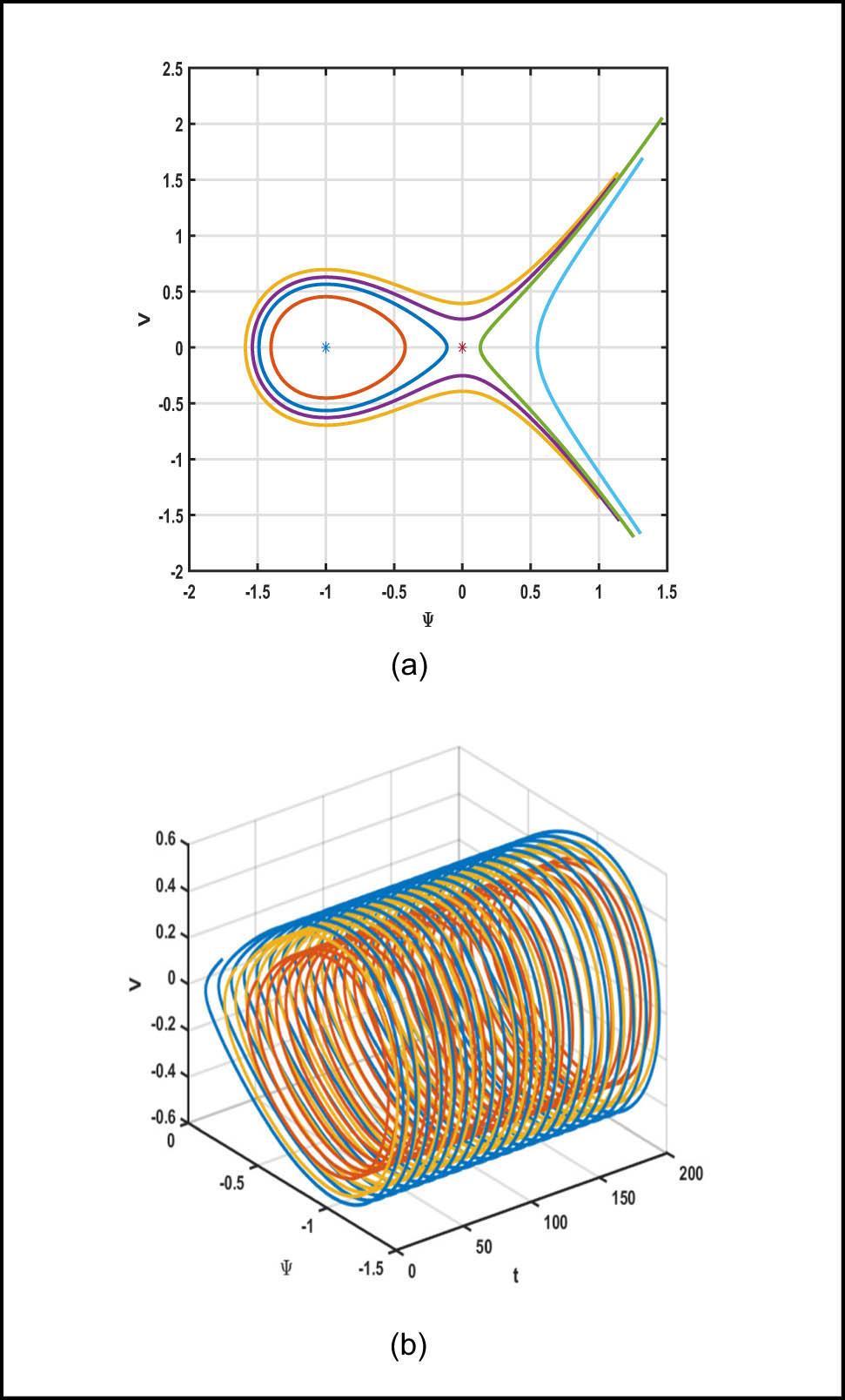
By employing analysis of vector fields in 2D dynamics, one can investigate the system’s (36) phase path. The phase trajectories of (36) vary depending on the selected nonzero parameters r 0 , r 1 , and r 2 . Notably, system (36) possesses two equilibria:

(38) M 1 = − r 1 − r 1 2 − 4 r 0 r 2 2 r 2 , 0 ,

(39) M 2 = − r 1 + r 1 2 − 4 r 0 r 2 2 r 2 , 0 .

To compute the Jacobian matrix of system (36), the following method can be utilized:

(40) J ( Ψ , V ) = 0 1 r 1 + 2 r 2 Ψ 0 = − r 1 − 2 r 2 Ψ .

By analyzing the equilibria ( M i ) in three different scenarios: while J ( Ψ , V ) = 0 , it becomes a cuspidal point; while J ( Ψ , V ) > 0 , it displays a center, suggesting that trajectories around this equilibrium are closed orbits, indicating periodic behavior. The system oscillates around the equilibrium without diverging or converging to it; and while J ( Ψ , V ) < 0 , it is identified as a saddle.This type of equilibrium is unstable, with trajectories moving towards it along some directions (stable manifold) and away from it along others (unstable manifold). To analyze system (36), we investigate how changes in parameters affect bifurcation. As a result, we reveal the influence of these changes by showing the system’s behavior through different parameter settings.

Setting the parameters of system (36) to fixed values leads to different classifications of the equilibrium points under various cases:

Case 1: With r 2 = − 1 , r 1 = 1 , and r 0 = 0.001 , the equilibrium M 2 is identified as a center, and M 1 as a saddle, as shown in Figure 6(a).

$Figure 6 The 2D (a) and 3D (b) phase orbits for case 1 are displayed. Equilibria are in star symbols, where M 2 {M}_{2} is identified as a center, and M 1 {M}_{1} as a saddle.$

Figure 6

The 2D (a) and 3D (b) phase orbits for case 1 are displayed. Equilibria are in star symbols, where M 2 is identified as a center, and M 1 as a saddle.

Case 2: With r 2 = 1 , r 1 = 1 , and r 0 = 0.001 , the equilibrium M 1 is identified as a center, and M 2 as a saddle, as depicted in Figure 7(a).

$Figure 7 The 2D (a) and 3D (b) phase orbits for case 2 are displayed. Equilibria are in star symbols, where M 1 {M}_{1} is identified as a center, and M 2 {M}_{2} as a saddle.$

Figure 7

The 2D (a) and 3D (b) phase orbits for case 2 are displayed. Equilibria are in star symbols, where M 1 is identified as a center, and M 2 as a saddle.

Case 3: With r 2 = 1 , r 1 = − 1 , and r 0 = 0.001 , the equilibrium M 2 is identified as a center, and M 1 as a saddle, as illustrated in Figure 8(a).

$Figure 8 The 2D (a) and 3D (b) phase orbits for case 3 are displayed. Equilibria are in star symbols, where M 2 {M}_{2} is identified as a center, and M 1 {M}_{1} as a saddle.$

Figure 8

The 2D (a) and 3D (b) phase orbits for case 3 are displayed. Equilibria are in star symbols, where M 2 is identified as a center, and M 1 as a saddle.

Case 4: With r 2 = − 1 , r 1 = − 1 , and r 0 = 0.001 , the equilibrium M 1 is identified as a center, and M 2 as a saddle, as demonstrated in Figure 9(a).

$Figure 9 The 2D (a) and 3D (b) phase orbits for case 4 are displayed. Equilibria are in star symbols, where M 1 {M}_{1} is identified as a center, and M 2 {M}_{2} as a saddle.$

Figure 9

The 2D (a) and 3D (b) phase orbits for case 4 are displayed. Equilibria are in star symbols, where M 1 is identified as a center, and M 2 as a saddle.

Figure 10(a) and (b) respectively display the maximum Lyapunov exponents when different initial conditions are taken. The initial values for Figure 10(a) is (1, 0.4), while for Figure 10(b), it is ( − 1 , 0.4). From the figures, we can observe that the maximum Lyapunov exponents at the central points are negative, indicating that the system is stable at these points. Here, we employ the maximum Lyapunov exponent as given by Rosenstein, for details, refer to [56].

$Figure 10 The maximum Lyapunov exponent when taking different initial values. For (a) k 0 = 0.001 {k}_{0}=0.001 , k 1 = 1 {k}_{1}=1 , k 2 = − 1 {k}_{2}=-1 , and for (b) k 0 = 0.001 {k}_{0}=0.001 , k 1 = 1 {k}_{1}=1 , k 2 = 1 {k}_{2}=1 .$

Figure 10

The maximum Lyapunov exponent when taking different initial values. For (a) k 0 = 0.001 , k 1 = 1 , k 2 = − 1 , and for (b) k 0 = 0.001 , k 1 = 1 , k 2 = 1 .

In the physical research of the GHRWE model, Figures 6–10 hold crucial significance. Figures 6–9 illustrate the classification of the system’s equilibrium points and the situations of the phase trajectories under different parameter settings. The existence of centers and saddle points reflects the different dynamic characteristics of the system under various parameter combinations. In the field of elasticity mechanics, this corresponds to the stable and unstable states of the hyperelastic rod under different loading and material parameter conditions. For example, in practical engineering, for flexible components such as the deployable arms and antennas of satellites, during different stages like launch, orbital operation, and working, the internal stress and strain distributions will change continuously. The analysis of the equilibrium points and phase trajectories in the GHRWE model can be analogized to the mechanical responses of these components under different working conditions, helping engineers understand their stability and potential deformation trends.

Figure 10, through the analysis of the maximum Lyapunov exponent, shows that the system is stable at the center, which provides a quantitative basis for judging the stability of the system at a specific point. When studying the wave propagation of the hyperelastic rod, a stable point means that the wave can propagate continuously and regularly in this state without sudden changes or instability. From an energy perspective, at the stable point, the transfer and distribution of energy are relatively balanced, while near the unstable points (such as around the saddle points), rapid changes and redistribution of energy will occur, which is closely related to the conversion of internal energy and wave propagation when the hyperelastic rod is under force. Taken together, these figures provide intuitive and crucial physical information for a deep understanding of the dynamic behavior of the hyperelastic rod described by the GHRWE model in elasticity mechanics, and contribute to predicting and optimizing the performance of hyperelastic materials in practical applications.

3.4 Sensitivity analysis with respect to initials

We explore how Eq. (36) reacts to changes in the initial value by examining the scenarios outlined in cases 1 and case 2. The outcomes are illustrated in Figure 11(a) and (b) with the system settings r 0 , r 1 , and r 2 arranged according to case 1. Similarly, Figure 12(a) and (b) present the results for the system settings configured as in case 2. The phase diagrams in Figures 11(b)–12(b) depict the scenario described by Eq. (36) under two distinct initial conditions. Conversely, Figures 11(a)–12(a) present the time series data for the system described by Eq. (36). The trajectories in blue illustrate the behavior, where Ψ is 0.25 or − 0.25 , V is 0.1, while trajectories in red reflect the circumstances for Ψ = ± 0.5 , V = 0.25 . The used times in sensitivity illustrations is t = [ 0 , 50 ] .

Figure 11

Sensitivity analysis for case 1: (a) time series and (b) phase orbits.

Figure 12

Sensitivity analysis for case 2: (a) time series and (b) phase orbits.

By studying trajectories from several initial setups, the effect of sensitivity can be assessed. This behavior is clearly demonstrated by the difference observed in Figures 11(a) and (b) and 12(a) and (b), where the blue and red curves are shown. The results clearly demonstrate that significant changes in the initial conditions profoundly affect the system’s behavior, provided that all other parameters remain constant.

Our research further explored how variations in parameters affect the system. This analysis is demonstrated by comparing Figures 11(a) and (b) with Figure 12(a) and (b). The findings reveal that the dynamic system is highly responsive to parameter variations, suggesting that even minor modifications can lead to considerable effects on the system’s performance.

Figures 11 and 12 display the time series and phase trajectories of the GHRWE model under different initial conditions. Their physical significance lies in revealing the sensitivity of the system to initial values. By comparing the curves under different initial conditions, it is clearly shown that a slight change in the initial values can significantly affect the system behavior. This is closely related to the fact that in practice, differences in the initial states of the hyperelastic rod lead to different dynamic responses. It provides a crucial basis for analyzing the mechanical properties of the hyperelastic rod described by the GHRWE model, such as the influence of different states at the initial stage of loading on subsequent fluctuations and stability.

3.5 Analysis of chaos

The interpretation of chaotic behaviors primarily revolves around the system’s unpredictable nature and extreme sensitivity to initial conditions over long time scales. This behavior arises from complex interactions within nonlinear dynamical systems, where even though the system follows deterministic mathematical rules, its behavior can exhibit seemingly random characteristics. The unpredictability in chaotic systems makes long-term prediction highly challenging, although short-term predictions remain feasible to some extent. Grasping the dynamic behaviors of system (7) is crucial. At this point, we thoroughly explores how Eq. (36) reacts to noise perturbations and evaluates its manifestation of chaotic behavior. The study utilizes the model below: Grasping the dynamic behaviors of system (7) is crucial. At this point, we thoroughly explores how Eq. (36) reacts to noise perturbations and evaluates its manifestation of chaotic behavior. The study utilizes the model below:

(41) Ψ ˙ = V , V ˙ = r 0 + r 1 Ψ + r 2 Ψ 2 + f sin ( ω 0 t ) .

To conduct the chaos evaluation, we will explore how sensitivity to noise varies from two angles. The analysis will concentrate on the variable f , representing the amplitude, and the variable ω 0 , representing the frequency. Modifying these factors will help us understand their impact on the system’s chaotic dynamics.

First, let us analyze how the amplitude parameter affects Eq. (36) with the frequency while keeping the frequency constant. Figure 13(a) and (b) present the simulation results, providing insights into how variations in the amplitude f influence the system.

Figure 13

Chaotic analysis for case 1: (a) the time series and (b) the phase orbits.

Next, the effect of the frequency parameter ω 0 on Eq. (36) is analyzed, with the amplitude f held constant. Figure 14(a) and (b) illustrate the results, shedding light on how changes in the frequency ω 0 impact the system.

Figure 14

In case 1, we examine the chaotic behavior of the system. (a) the time series and (b) the phase plot.

Under the same experimental conditions as in case 1, starting from (0.25, 0.2), Figure 13(a) and (b) analyze the system’s response with a fixed frequency of ω 0 = π and no amplitude. The results are shown by the blue line, which depicts the system’s time progression and phase trajectories. Following this, scenarios with amplitude value 0.2 (red curve) and 0.4 (yellow curve) are considered. The distinct divergence of the blue line from the other curves emphasizes the presence of significant chaotic dynamics and highlights the system’s sensitivity to variations in amplitude.

The impact of frequency ω 0 on the dynamic system is assessed through the results shown in Figure 14(a) and (b). Starting with f = 0 , the simulation results for time series and phase orbits are illustrated by the blue curve. The red curve represents the scenario with f = 0.2 and ω 0 = π , whereas the yellow curve depicts the case with f = 0.2 and ω 0 = 2 π . The differences observed underscore the existence of chaotic dynamics within the system. In addition, the dynamic system shows significant sensitivity to variations in the frequency ω 0 .

Figures 13 and 14 are used to analyze the chaotic behavior of the GHRWE model. By changing the amplitude and the frequency of the noise perturbation, they present the changes in the time series and phase trajectories of the system under different parameters. Their physical significance lies in revealing the sensitivity of the system to noise and the characteristics of chaotic dynamics. This helps to understand the uncertainty and complexity of the dynamic behavior of the hyperelastic rod in complex and disturbed real-world environments, such as when it is subjected to external random forces. It provides an important reference for studying the mechanical properties of the hyperelastic rod described by the GHRWE model under nonideal conditions.

3.6 Numerical results

In the realm of numerical analysis, the derivation of numerical solutions can be approached through various methodologies. One such approach is to furnish approximate analytical solutions, which are often derived through sophisticated decomposition techniques. Notably, the adomian decomposition method (ADM) and its variant, the modified adomian decomposition method, are frequently employed for this purpose. In addition, the reduced differential transform method and the residual power series method are also recognized for their efficacy in yielding approximate solutions. For a comprehensive discourse on these approximate solutions, the reader is directed to the relevant literature [57–60].

Conversely, an alternative strategy involves the direct computation of numerical results. In the present study, we have opted to employ the Chebyshev spectral collocation method to obtain the numerical results. This method is chosen for its demonstrated accuracy and efficiency in approximating solutions to differential equations.

In this part, we will verify the analytical results that were obtained in the previous part with the Chebyshev spectral collocation method. The Chebyshev nodes we used in this part are x k = cos ( k π n ) , k = 0 , 1 , … , n . For the nonlinear terms Ψ 3 ( ξ ) of Eq. (8), we use Newton iteration method to handle, and then we have the following iterative relation.

(42) D ( 2 ) Ψ → k − diag ( r 1 − 2 r 2 Ψ → k ) ⋅ Ψ → k = r 0 − r 2 Ψ → k − 1 2 ,

where Ψ → = ( Ψ ( ξ 1 ) , Ψ ( ξ 2 ) , … , Ψ ( ξ n ) ) T and D ( 2 ) represents the corresponding differentiation matrices of the second-order derivative d 2 Ψ ( ξ ) d ξ 2 , which can be obtained analytically. The differential matrices corresponding of the first-order derivative, we denote it as D ( 1 ) and can be calculated according to the following format. c 1 = c n = 2 and c 2 = … = c n − 1 = 1 .

(43) D i , j ( 1 ) = c i ( − 1 ) j + i c j ( x i − x j ) , j ≠ i − 1 2 x i ( 1 − x i 2 ) , j = i ≠ 1 , n 2 ( n − 1 ) 2 + 1 6 , j = i = 1 − 2 ( n − 1 ) 2 + 1 6 , j = i = n .

By combining the representation form of D ( 1 ) , we have D ( 2 ) = ( D ( 1 ) ) 2 . For more detailed discussion about the Chebyshev spectral method, one can refer to [61,62].

The initial and boundary conditions are constrained by the exact solution U 4 ( x , t ) or U 9 ( x , t ) , which we will discuss in the following part. We denote the boundary conditions as Ψ ( ξ 0 ) = g 1 and Ψ ( ξ n ) = g 2 . When dealing with boundary conditions, we denote them as L 1 Ψ → = g 1 and L 2 Ψ → = g 2 separately.

At each step of the iteration process, we have

(44) L k Ψ → k = f k ,

where

(45) L k = D ( 2 ) − diag ( r 1 − 2 r 2 Ψ → k ) L 1 L 2 ,

(46) f k = r 0 − r 2 Ψ → k − 1 2 g 1 g 2 .

During the iteration process, we set the starting numerical solution is Ψ → 0 = ( 0 , 0 , … , 0 ) T . The upper limit of error for iteration termination is ∣ Ψ → k − Ψ → k − 1 ∣ < 1 0 − 9 . After we obtain the numerical results at the Chebyshev nodes, the cubic b-spline method was applied to obtain the numerical results at other points.

Numerical results for case one: U 4 ( x , t ) , α = 1.1 , β = 0.6 , σ = 1 , μ = 5 , τ = − 1.5 , λ = 0.5 , θ = 0.5 , C 1 = 1 , C 2 = 100 , a = 0.1 , and b = 0.09 .

Table 1 and Figure 14 present the comparison between the analytical results and the numerical results. From Table 1 and Figure 14(a), the numerical solutions with the method we proposed are in excellent agreement with the analytical solutions. Figure 14(b) shows the comparison between the numerical results and the analytical results when the variable t is fixed at 1.2. Figure 14(b) is a slice of Figure 14(a) at t = 1.2 , these results also show that the numerical solution and analytical solution are in good agreement.

Table 1

Comparison between the numerical solution U ˆ 4 ( x , t ) and the analytical solution U 4 ( x , t ) at t = 1.2

x	U ˆ 4 ( x , 1.2 )	U 4 ( x , 1.2 )	∣ U ˆ 4 ( x , 1.2 ) − U 4 ( x , 1.2 ) ∣
− 1.8	− 0.862768833	− 0.862768833	1.25471 × 1 0 − 10
− 1.4	− 0.859578503	− 0.859578503	3.09457 × 1 0 − 10
− 1.0	− 0.855150759	− 0.855150759	4.68218 × 1 0 − 10
− 0.6	− 0.849493461	− 0.849493461	4.01097 × 1 0 − 10
− 0.2	− 0.842616628	− 0.842616628	2.67031 × 1 0 − 12
0.2	− 0.834532395	− 0.834532396	6.43600 × 1 0 − 10
0.6	− 0.825254972	− 0.825254973	4.25045 × 1 0 − 10
1.0	− 0.81480059	− 0.81480059	1.15692 × 1 0 − 10
1.4	− 0.803187435	− 0.803187436	5.76932 × 1 0 − 10
1.8	− 0.790435594	− 0.790435595	2.79924 × 1 0 − 10

Numerical results for case two: U 9 ( x , t ) , α = 1.1 , β = 0.3 , σ = 1 , μ = 5 , τ = − 1.8 , λ = 0.5 , θ = 0.5 , C 1 = 1 , C 2 = 100 , a = 0.1 , b = 0.09 .

$Figure 15 (a) The absolute error between numerical and analytical results of U 4 ( x , t ) {U}_{4}\left(x,t) , where x ∈ [ − 2 , 2 ] x\in \left[-2,2] and t ∈ [ 0 , 2 ] t\in \left[0,2] and (b) ∣ U 4 ( x , t ) ∣ | {U}_{4}\left(x,t)| and ∣ U ˆ 4 ( x , t ) ∣ | {\hat{U}}_{4}\left(x,t)| at t = 1.2 t=1.2 , where x ∈ [ − 2 , 2 ] x\in \left[-2,2] .$

Figure 15

(a) The absolute error between numerical and analytical results of U 4 ( x , t ) , where x ∈ [ − 2 , 2 ] and t ∈ [ 0 , 2 ] and (b) ∣ U 4 ( x , t ) ∣ and ∣ U ˆ 4 ( x , t ) ∣ at t = 1.2 , where x ∈ [ − 2 , 2 ] .

Table 2 and Figure 15 present the comparison between the analytical results U 9 ( x , t ) and the numerical results U ˆ 9 ( x , t ) . Figure 15(b) is a slice of Figure 15(a) at t = 1 . These numerical results demonstrate both overall and slice wise that our numerical method has high accuracy (Figure 16).

Table 2

Comparison between the numerical solution U ˆ 9 ( x , t ) and the analytical solution U 9 ( x , t ) at t = 1

x	U ˆ 9 ( x , 1.0 )	U 9 ( x , 1.0 )	∣ U ˆ 9 ( x , 1.0 ) − U 9 ( x , 1.0 ) ∣
− 0.9	0.902897235	0.902897238	2.71634 × 1 0 − 9
− 0.7	0.634193693	0.634193759	6.67262 × 1 0 − 8
− 0.5	0.38032516	0.380325155	4.91564 × 1 0 − 9
− 0.3	0.158580563	0.158580339	2.24018 × 1 0 − 7
− 0.1	− 0.013485201	− 0.013485617	4.15769 × 1 0 − 7
0.1	− 0.120680524	− 0.120680771	2.46524 × 1 0 − 7
0.3	− 0.152849499	− 0.152849501	1.30237 × 1 0 − 9
0.5	− 0.106840587	− 0.106840852	2.64920 × 1 0 − 7
0.7	0.012853578	0.012853252	3.25437 × 1 0 − 7
0.9	0.195003973	0.195003957	1.52550 × 1 0 − 8

$Figure 16 (a) The absolute error between numerical and analytical results of U 9 ( x , t ) {U}_{9}\left(x,t) , where x ∈ [ − 1 , 1 ] x\in \left[-1,1] and t ∈ [ 0 , 2 ] t\in \left[0,2] and (b) ∣ U 9 ( x , t ) ∣ | {U}_{9}\left(x,t)| and ∣ U ˆ 9 ( x , t ) ∣ | {\hat{U}}_{9}\left(x,t)| at t = 1.0 t=1.0 , where x ∈ [ − 1 , 1 ] x\in \left[-1,1] .$

Figure 16

(a) The absolute error between numerical and analytical results of U 9 ( x , t ) , where x ∈ [ − 1 , 1 ] and t ∈ [ 0 , 2 ] and (b) ∣ U 9 ( x , t ) ∣ and ∣ U ˆ 9 ( x , t ) ∣ at t = 1.0 , where x ∈ [ − 1 , 1 ] .

4 Conclusions

4.1 The overall advantages of this article

The method employed in our study, which combines the Hamiltonian structure and modified G ′ G 2 -expansion method within the framework of planar dynamical systems, offers several notable advantages.

First and foremost, our approach provides a comprehensive and systematic framework for examining the GHRWE. Traditionally, constructing a Hamiltonian framework for Eq. (5) within the context of GHRWE has been deemed infeasible. However, drawing from our pioneering work, we have successfully employed the trial equation technique to modify Eq. (5), resulting in an equivalent formulation, Eq. (7), which is a novel approach not previously addressed in the literature [42–44]. This modification is not just a theoretical advancement; it is a practical one as well. By establishing a Hamiltonian framework, we can tap into the rich body of knowledge that Hamiltonian mechanics provides, particularly regarding the principle of energy conservation. This principle allows us to analyze the dynamics of the system with precision, focusing on the trajectories of energy within the system. This approach not only enhances our understanding of the underlying dynamics but also equips professionals with a valuable tool for assessing energy-related aspects of their specific challenges. Furthermore, it opens up new avenues for research, as it offers a structured way to study the complex interplay of fractal and chaotic dynamics within the GHRWE, which is critical for understanding the full spectrum of nonlinear phenomena present in such systems.

Secondly, we have employed the modified G ′ G 2 -expansion method, which has enabled us to derive a range of wave solutions, from diverse waveforms to solitons. This capability provides us with the flexibility necessary to represent various soliton propagation scenarios. Such versatility is an invaluable asset for those assessing the variations in soliton types and characteristics within GHRWE systems. By offering a broad spectrum of solutions, this method not only enhances our understanding of the underlying dynamics but also equips researchers and engineers with a powerful tool for analyzing and predicting the behavior of complex wave phenomena in GHRWE systems. This comprehensive approach to solution generation is indeed a significant contribution of our research, highlighting the potential of the method in addressing the multifaceted nature of nonlinear wave dynamics.

Building upon our exploration of the impact of different fractional-order derivative forms on solutions, our research delves into the nuances that these derivatives introduce to the system’s dynamics. Fractional calculus, which deals with integrals and derivatives of noninteger order, has gained increasing recognition for its ability to model complex systems with memory and nonlocality effects that traditional integer-order calculus cannot fully capture. Our comparative analysis has revealed how these fractional derivatives, with their inherent nonlocal properties, can significantly alter the system’s behavior, particularly in the context of nonlinear phenomena and soliton propagation. This insight is crucial for advancing our understanding of complex systems, as it allows us to account for the long-term dependencies and hereditary properties that are often present in real-world applications. By doing so, our work not only fills a gap in the existing literature [42–44] but also paves the way for more sophisticated modeling techniques that can better predict and control system transitions and instabilities within the GHRWE. This enhanced predictive capability is a significant stride towards managing the intricacies of nonlinear dynamics in practical applications.

Finally, we have particularly emphasized the importance of verifying the accuracy of our analytical solutions to the equation. To this end, we have employed the Chebyshev spectral collocation method, which is renowned for its high precision and numerical stability. Through this method, we have conducted a detailed comparison between the partial analytical solutions obtained in the previous section and the numerical solutions. We calculated the errors between the two. The results show that the errors between our analytical solutions and numerical solutions are extremely small, which verifies the high precision of our analytical solutions. This finding not only confirms the effectiveness of our method but also provides a solid foundation for subsequent theoretical research and practical applications. Moreover, this high-precision verification process itself is a highlight of this study, demonstrating the potential and reliability of our method in dealing with nonlinear complex dynamic systems.

4.2 Underlying shortcomings of this article

Although this article boasts numerous benefits, it comes with specific constraints that users should consider for its practical use.

A significant limitation lies in the complexity of the mathematical model we employ. Utilizing the Hamiltonian alongside the modified G ′ G 2 -expansion technique demands a robust mathematical foundation, potentially hindering accessibility for individuals lacking advanced mathematical skills. Nevertheless, we have endeavored to enhance the approach’s comprehensibility with concise explanations and practical examples.

Another consideration is the computational intensity associated with numerical simulations. Depending on the problem’s complexity and the available computing resources, running simulations can be time consuming and resource–intensive. Engineers and researchers should be prepared for this aspect and allocate sufficient computational resources accordingly.

The computational demands of numerical modeling are also a factor to consider. The time and resources required for simulations can vary significantly with the intricacy of the problem and the computational assets at hand. It is crucial for professionals to anticipate this and ensure they have adequate computational capacity for their needs.

Summing up, our technique presents a robust and adaptable framework for examining GHRWE, excelling in energy preservation, evaluating the stability of critical points, and deriving wave solutions. Although it might entail complexity and computational effort, its practical value is underscored by its capacity to shed light on system dynamics, stability, and soliton dynamics. We anticipate that this overview of the method’s advantages and limitations will guide readers in effectively harnessing it for their own challenges across various fields.

4.3 Achievements and future outlook

In our research, we have successfully implemented the enhanced G ′ G 2 -expansion technique to dissect the GHRWE, uncovering a plethora of precise solutions. Upon examining the architecture of Eq. (5), it is evident that crafting a Hamiltonian framework for the exploration of nonlinear dynamics presents a formidable challenge. However, the pivotal innovation of this article lies in the innovative application of the trial equation method, which has facilitated the transformation of Eq. (5) into a novel configuration. This transformation has been instrumental in establishing the Hamiltonian system framework essential for the analysis of GHRWE. This novel approach has not been previously explored in existing scholarly works [42–44].

Our research methodology has not only achieved a theoretical breakthrough but also demonstrated its unique value in practical applications. Compared to the previous studies, our method shows clear advantages and innovativeness in the following aspects:

Establishment of the Hamiltonian framework: In the study of nonlinear dynamics, the establishment of a Hamiltonian framework has always been a challenge. By applying the trial equation method, we have successfully transformed Eq. (5) into a new form suitable for Hamiltonian analysis, which has not been attempted in previous studies [42– 44].
Pioneering new research areas: Our method allows us to delve into areas such as phase diagrams, bifurcation scenarios, sensitivity analyses concerning initial conditions, and the examination of chaotic behaviors–all of which have been absent in the existing literature [42– 44].
Impact analysis of fractional derivative forms: We have also conducted a comparative analysis of the impact of various fractional derivative forms on the solutions, an aspect that has similarly not been addressed in prior studies [42– 44].
Precise verification of analytical solutions: We have emphasized the importance of validating the precision of our analytical solutions for the equation. By harnessing the power of the Chebyshev spectral collocation method, an approach celebrated for its exceptional accuracy and numerical robustness, we have meticulously compared the partial analytical solutions derived in the preceding sections with their numerical counterparts, quantifying the discrepancies between them. The findings reveal that the discrepancies are minuscule, thereby affirming the high fidelity of our analytical solutions.

Through these comparisons, it is evident that our research provides not only new perspectives and methods on a theoretical level but also demonstrates significant potential and reliability in practical applications. Our work not only fills the gaps in the existing literature but also offers new directions and tools for future research, which is of great importance in advancing scientific inquiry and the discovery of new knowledge.

We have underscored the critical role of validating the precision of our analytical solutions for the equation. To achieve this, we have harnessed the power of the Chebyshev spectral collocation method, an approach celebrated for its exceptional accuracy and numerical robustness. By utilizing this technique, we have meticulously compared the partial analytical solutions derived in the preceding sections with their numerical counterparts, quantifying the discrepancies between them. The findings reveal that the discrepancies are minuscule, thereby affirming the high fidelity of our analytical solutions.

This significant outcome not only substantiates the efficacy of our methodology but also lays a robust groundwork for future theoretical explorations and practical implementations. The meticulous verification process itself is a notable accomplishment of this research, underscoring the method’s potential and dependability in addressing the complexities of nonlinear dynamic systems. By extending the scope of our investigation, we have not only enriched the theoretical understanding of the GHRWE but also provided a powerful analytical tool that can be applied to a broader spectrum of nonlinear dynamical systems. Our findings not only deepen the comprehension of GHRWE but also demonstrate the applicability and effectiveness of our analytical method in dealing with complex nonlinear phenomena. These results contribute new perspectives and potential applications to the ongoing discourse in the field, potentially stimulating further developments in related areas of research. This work stands as a testament to the importance of innovative methodologies in pushing the boundaries of scientific inquiry and underscores the value of interdisciplinary approaches in the pursuit of new knowledge. Our research not only offers in-depth theoretical insights into GHRWE but also provides a reliable analytical framework for the study of nonlinear dynamics through precise analytical solutions and numerical validation.

In our forthcoming research, we are contemplating the extension of the polynomial in Eq. (16) to a rational function format:

(47) U ( ξ ) = a 0 + a 1 G ′ G 2 + a 2 G ′ G 2 2 + b 1 G ′ G 2 − 1 + b 2 G ′ G 2 − 2 c 0 + c 1 G ′ G 2 + c 2 G ′ G 2 2 + d 1 G ′ G 2 − 1 + d 2 G ′ G 2 − 2 ,

where the coefficients a 0 , a 1 , a 2 , b 1 , b 2 , c 0 , c 1 , c 2 , d 1 , and d 2 are to be determined subsequently. The enhanced complexity of Eq. (47) in contrast to Eq. (16) suggests that by substituting the rational expression of U ( ξ ) back into the original equation, we may achieve more precise solutions, potentially uncovering additional soliton solutions. While these computations are expected to be more intricate, we are committed to venturing down this path with determination in our future work. Moreover, we aim to apply the research results to more practical scenarios in the future, such as the mechanical analysis of artificial hyperelastic tissues in biomedical engineering and the design and optimization of new hyperelastic material structures in the aerospace field. This will expand the application scope of the GHRWE model and promote the development of interdisciplinary research.

Funding information: The work presented in this article was supported by the scientific research project of Shanghai Dianji University (23B0405).
Author contributions: Hongwei Ma: writing – original draft, validation, supervision, writing – review, editing. Ziming Liu: formal analysis, method-conclusion. Yiqun Sun: writing – original draft. Peng Guo: conceptualization, supervision. Jianming Qi: writing – review, editing. All authors have accepted responsibility for the entire content of this manuscript and approved its submission.
Conflict of interest: The authors state no conflict of interest.
Data availability statement: Data sharing is not applicable to this article as no data sets were generated or analyzed during the current study.

References

[1] Iqbal MS, Seadawy AR, Baber MZ, Qasim M. Application of modified exponential rational function method to Jaulent-Miodek system leading to exact classical solutions. Chaos Soliton Fract. 2022;164:112600. 10.1016/j.chaos.2022.112600Search in Google Scholar

[2] Iqbal MS, Seadawy AR, Baber MZ. Demonstration of unique problems from Soliton solutions to nonlinear Selkov-Schnakenberg system. Chaos Soliton Fract. 2022;162:112485. 10.1016/j.chaos.2022.112485Search in Google Scholar

[3] Tajadodi H, Khan ZA, Irshad AR, Gómez-Aguilar JF, Khan A, Khan H. Exact solutions of conformable fractional differential equations. Results Phys. 2021;22:103916. 10.1016/j.rinp.2021.103916Search in Google Scholar

[4] Kaplan M, Butt AR, Thabet H, Akbulut A, Raza N, Kumar D. An effective computational approach and sensitivity analysis to pseudo-parabolic-type equations. Wave Random Complex. 2021;34(5):4172–86. 10.1080/17455030.2021.1989081Search in Google Scholar

[5] Az-Zo’bi EA, Akinyemi L, Alleddawi AO. Construction of optical solitons for conformable generalized model in nonlinear media. Mod Phys Lett B. 2021;35:2150409. 10.1142/S0217984921504091Search in Google Scholar

[6] Az-Zo’bi EA, Dawoud KA, Marashdeh M. Numeric-analytic solutions of mixed-type systems of balance laws. Appl Math Comput. 2015;265:133–43. 10.1016/j.amc.2015.04.119Search in Google Scholar

[7] Inc M, Az-Zo’bi EA, Jhangeer A, Rezazadeh H, Ali MN, Kaabar MKA. New soliton solutions for the higher-dimensional non-local Ito equation. Nonlinear Eng. 2021;10(1):374–84. 10.1515/nleng-2021-0029Search in Google Scholar

[8] Iqbal M, Alam MN, Lu D, Seadawy A, Alsubaie NE, Ibrahim S. On the exploration of dynamical optical solitons to the modify unstable nonlinear Schrödinger equation arising in optical fbers. Opt Quantum Electron. 2024;56:765. 10.1007/s11082-024-06468-7Search in Google Scholar

[9] Taghizadeh N, Mirzazadeh M. The direct algebraic method to complex nonlinear partial differential equations. Int J Appl Math Comput. 2013;5(3):12–6. Search in Google Scholar

[10] Sulaiman TA, Bulut H, Yokus A, Baskonus HM. On the exact and numerical solutions to the coupled Boussinesq equation arising in ocean engineering. Indian J Phys. 2019;93:647–56. 10.1007/s12648-018-1322-1Search in Google Scholar

[11] Hirota R. The direct method in soliton theory. CUP. 2004;155:1–200. 10.1017/CBO9780511543043Search in Google Scholar

[12] Seadawy AR, Younis M, Baber MZ, Rizvi STR, Iqbal MS. Diverse acoustic wave propagation to confirmable time-space fractional KP equation arising in dusty plasma. Commun Theor Phys. 2021;73(11):115004. 10.1088/1572-9494/ac18bbSearch in Google Scholar

[13] Soliman AA. The modified extended direct algebraic method for solving nonlinear partial differential equations. Int J Nonlinear Sci. 2008;6(2):136–44. Search in Google Scholar

[14] Cheemaa N, Younis M. New and more general traveling wave solutions for nonlinear Schrödinger equation. Wave Random Complex. 2016;26(1):30–41. 10.1080/17455030.2015.1099761Search in Google Scholar

[15] Yao SW, Behera S, Inc M, Rezazadeh H, Virdi JPS, Mahmoud W, et al. Analytical solutions of conformable Drinfelad-Sokolov-Wilson and Boiti Leon Pempinelli equations via sine-cosine method. Results Phys. 2022;42:105990. 10.1016/j.rinp.2022.105990Search in Google Scholar

[16] Feng Q. A new approach for seeking coefficient function solutions of conformable fractional partial differential equations based on the Jacobi elliptic equation. Chin J Phys. 2018;56(6):2817–28. 10.1016/j.cjph.2018.08.006Search in Google Scholar

[17] Cohen D, Raynaud X. Geometric finite difference schemes for the generalized hyperelastic-rod wave equation. J Comput Appl Math. 2011;235(8):1925–40. 10.1016/j.cam.2010.09.015Search in Google Scholar

[18] Tian C, Yan W, Zhang H. The Cauchy problem for the generalized hyperelastic rod wave equation. Math Nachr. 2014;287(17–18):2116–37. 10.1002/mana.201200243Search in Google Scholar

[19] Lv N, Li J, Yuan X, Wang R. Controllable rogue waves in a compressible hyperelastic plate. Phys Lett A. 2023;461:128639. 10.1016/j.physleta.2023.128639Search in Google Scholar

[20] Demray ŞT. Solutions for KMM System and generalized hyperelastic-rod wave equation. OKÜ Fen Bil. Ens. Dergisi. 2022;5(3):1690–703. 10.47495/okufbed.1164007Search in Google Scholar

[21] Novruzov E, Bayrak V. Blow-up criteria for a two-component nonlinear dispersive wave system. J Funct Anal. 2022;282(12):109454. 10.1016/j.jfa.2022.109454Search in Google Scholar

[22] Houwe A, Abbagari S, Akinyemi L, Saliou Y, Justin M, Doka SY. Modulation instability, bifurcation analysis and solitonic waves in nonlinear optical media with odd-order dispersion. Phys Lett A. 2023;488:129134. 10.1016/j.physleta.2023.129134Search in Google Scholar

[23] Akinyemi L, Houwe A, Abbagari S, Wazwaz AM, Alshehri HM, Osman MS. Effects of the higher-order dispersion on solitary waves and modulation instability in a monomode fiber. Optik. 2023;288:171202. 10.1016/j.ijleo.2023.171202Search in Google Scholar

[24] Mathanaranjan T, Hashemi MS, Rezazadeh H, Akinyemi L, Bekir A. Chirped optical solitons and stability analysis of the nonlinear Schrödinger equation with nonlinear chromatic dispersion. Commun Theor Phys. 2023;75(8):085005. 10.1088/1572-9494/ace3b0Search in Google Scholar

[25] Akinyemi L, Rezazadeh H, Yao SW, Akbar MA, Khater MMA, Jhangeer A, et al. Nonlinear dispersion in parabolic law medium and its optical solitons. Results Phys. 2021;26:104411. 10.1016/j.rinp.2021.104411Search in Google Scholar

[26] Debin K, Rezazadeh H, Ullah N, Vahidi J, Tariq KU, Akinyemi L. New soliton wave solutions of a (2+1)-dimensional Sawada-Kotera equation. 2023;8(5):527–32. 10.1016/j.joes.2022.03.007Search in Google Scholar

[27] Wazwaz AM, Kaur L. Optical solitons and Peregrine solitons for nonlinear Schrödinger equation by variational iteration method. Optik. 2019;179:804–9. 10.1016/j.ijleo.2018.11.004Search in Google Scholar

[28] Wazwaz AM, Kaur L. Optical solitons for nonlinear Schrödinger (NLS) equation in normal dispersive regimes. Optik. 2019;184:428–35. 10.1016/j.ijleo.2019.04.118Search in Google Scholar

[29] Kaur L, Wazwaz AM. Bright-dark optical solitons for Schrödinger-Hirota equation with variable coefficients. Optik. 2019;179:479–84. 10.1016/j.ijleo.2018.09.035Search in Google Scholar

[30] Wazwaz AM, Kaur L. New integrable Boussinesq equations of distinct dimensions with diverse variety of soliton solutions. Nonlinear Dyn. 2019;97:83–94. 10.1007/s11071-019-04955-1Search in Google Scholar

[31] Raut S, Saha S, Das AN, Talukder P. Complete discrimination system method for finding exact solutions, dynamical properties of combined Zakharsov-Kuznetsov-modified Zakarsov-Kuznetsov equation. Alex Eng J. 2023;76:247–57. 10.1016/j.aej.2023.06.020Search in Google Scholar

[32] Raut S, Barman R, Sarkar T. Integrability, breather, lump and quasi-periodic waves of non-autonomous Kadomtsev-Petviashvili equation based on Bell-polynomial approach. Wave Motion. 2023;119:103125. 10.1016/j.wavemoti.2023.103125Search in Google Scholar

[33] Raut S, Ma WX, Barman R, Roy S. A non-autonomous Gardner equation and its integrability: Solitons, positons and breathers. Chaos Soliton Fract. 2023;176:114089. 10.1016/j.chaos.2023.114089Search in Google Scholar

[34] Raut S, Roy S, Saha S, Saha S, Das AN. Effect of kinematic viscosity on ion acoustic waves in superthermal plasma comprising cylindrical and spherical geometry. Int J Appl Comput Math. 2022;8(4):196. 10.1007/s40819-022-01418-xSearch in Google Scholar

[35] Roy S, Raut S, Kairi RR, Chatterjee P. Bilinear Bäcklund, Lax pairs, breather waves, lump waves and soliton interaction of (2+1)-dimensional non-autonomous Kadomtsev-Petviashvili equation. Nonlinear Dyn. 2023;111(6):5721–41. 10.1007/s11071-022-08126-7Search in Google Scholar

[36] Sarkar T, Roy S, Raut S, Mali PC. Studies on the dust acoustic shock, solitary, and periodic waves in an unmagnetized viscous dusty plasma with two-temperature ions. Braz J Phys. 2023;53(1):12. 10.1007/s13538-022-01221-5Search in Google Scholar

[37] Mahdy AMS. Stability, existence, and uniqueness for solving fractional glioblastoma multiforme using a Caputo-Fabrizio derivative. Math Meth Appl Sci. 2025;48(7):7360–77. 10.1002/mma.9038Search in Google Scholar

[38] Morales-Delgado VF, Gómez-Aguilar JF, Escobar-Jiménez RF, Taneco-Hernández MA. Fractional conformable derivatives of Liouville-Caputo type with low-fractionality. Phys A. 2018;503:424–38. 10.1016/j.physa.2018.03.018Search in Google Scholar

[39] Pérez JES, Gómez-Aguilar JF, Baleanu D, Tchier F. Chaotic attractors with fractional conformable derivatives in the Liouville-Caputo sense and its dynamical behaviors. Entropy-Switz. 2018;20(5):384. 10.3390/e20050384Search in Google Scholar PubMed PubMed Central

[40] Yépez-Martínez H, Gómez-Aguilar J F, Atangana A. First integral method for non-linear differential equations with conformable derivative. Math. Model. Nat Phenom. 2018;13(1):14. 10.1051/mmnp/2018012Search in Google Scholar

[41] Yao SW, Shahzad T, Ahmed MO, Baber MZ, Iqbal MS, Inc M. Extraction of soliton solutions for the time-space fractional order nonclassical Sobolev-type equation with unique physical problems. Results Phys. 2023;45:106256. 10.1016/j.rinp.2023.106256Search in Google Scholar

[42] Shahzad T, Ahmad MO, Baber MZ, Ahmed N, Ali SM, Akgül A, et al. Extraction of soliton for the confirmable time-fractional nonlinear Sobolev-type equations in semiconductor by phi6-modal expansion method. Results Phys. 2023;46:106299. 10.1016/j.rinp.2023.106299Search in Google Scholar

[43] Simbanefayi I, Gandarias ML, Khalique CM. Travelling wave solutions, symmetry reductions and conserved vectors of a generalized hyper-elastic rod wave equation. Partial Differ Equ Appl Math. 2023;7:100501. 10.1016/j.padiff.2023.100501Search in Google Scholar

[44] Shahzad T, Ahmad MO, Baber MZ, Ahmed M, Akgül A, Abdeljawad T, et al. Explicit solitary wave structures for the fractional-order Sobolev-type equations and their stability analysis. Alex Eng J. 2024;92:24–38. 10.1016/j.aej.2024.02.032Search in Google Scholar

[45] Han TY, Li Z, Li CY. Bifurcation analysis, stationary optical solitons and exact solutions for generalized nonlinear Schrödinger equation with nonlinear chromatic dispersion and quintuple power-law of refractive index in optical fibers. Phys A. 2023;615:128599. 10.1016/j.physa.2023.128599Search in Google Scholar

[46] Han TY, Jiang YY, Lyu JJ. Chaotic behavior and optical soliton for the concatenated model arising in optical communication. Results Phys. 2024;58:107467. 10.1016/j.rinp.2024.107467Search in Google Scholar

[47] Qiii JM, Cui QH, Bai LQ, Sun YQ. Investigating exact solutions, sensitivity, and chaotic behavior of multi-fractional order stochastic Davey-Sewartson equations for hydrodynamics research applications. Chaos Soliton Fract. 2024;180:114491. 10.1016/j.chaos.2024.114491Search in Google Scholar

[48] Qi JM, Wang X, Sun YQ. Investigating bifurcation and Chaos in lossy electrical transmission line models with Hamiltonian dynamics. Nonlinear Dyn. 2024;112:17551–84. 10.1007/s11071-024-09981-2Search in Google Scholar

[49] Altawallbeh Z, Az-Zo’bi E, Alleddawi OA, Šenol M, Akinyemi L Novel liquid crystals model and its nematicons. Opt Quantum Electron. 2022;54:861. 10.1007/s11082-022-04279-2Search in Google Scholar

[50] Alam MN. Exact solutions to the foam drainage equation by using the new generalized G′G-expansion method. Results Phys. 2015;5:168–77. 10.1016/j.rinp.2015.07.001Search in Google Scholar

[51] Shakeel M, Zafar A, Alameri A, Rehman MJU, Awrejcewicz J, Umer M, et al. Noval soliton solution, sensitivity and stability analysis to the fractional gKdV-ZK equation. Sci Rep. 2024;14:3770. 10.1038/s41598-024-51577-8Search in Google Scholar PubMed PubMed Central

[52] Saboor A, Shakeel M, Liu X, Zafar A, Ashraf M. A comparative study of two fractional nonlinear optical model via modifed G′G2-expansion method. Opt Quantum Electron. 2024;56:259. 10.1007/s11082-023-05824-3Search in Google Scholar

[53] Alam MN, Rahman MA. Study of the parametric effect of the wave profiles of the time-space fractional soliton neuron model equation arising in the topic of neuroscience. Partial Differ Equ Appl Math. 2024;12:100985. 10.1016/j.padiff.2024.100985Search in Google Scholar

[54] Alam MN, Iqbal M, Hassan M, Fayz-Al-Asad M, Hossain MS, Tunç C. Bifurcation, phase plane analysis and exact soliton solutions in the nonlinear Schrödinger equation with Atanganaas conformable derivative. Chaos Soliton Fract. 2024;182:114724. 10.1016/j.chaos.2024.114724Search in Google Scholar

[55] Ali AR, Alam MN, Parven MW. Unveiling optical soliton solutions and bifurcation analysis in the space-time fractional Fokas-Lenells equation via SSE approach. Sci Rep. 2024;14:2000. 10.1038/s41598-024-52308-9Search in Google Scholar PubMed PubMed Central

[56] Rosenstein MT, Collins JJ, Luca CJD. A practical method for calculating largest Lyapunov exponents from small data sets. Phys D. 1993;65(1–2):117–34. 10.1016/0167-2789(93)90009-PSearch in Google Scholar

[57] Az-Zo’bi EA. Construction of solutions for mixed hyperbolic elliptic Riemann initial value system of conservation laws. Appl Math Model. 2013;37(8):6018–24. 10.1016/j.apm.2012.12.006Search in Google Scholar

[58] Az-Zo’bi EA. On the reduced differential transform method and its application to the generalized Burgers-Huxley equation. Appl Math Sci. 2014;8:8823–31. 10.12988/ams.2014.410835Search in Google Scholar

[59] Az-Zo’bi EA. Exact analytic solutions for nonlinear diffusion equations via generalized residual power series method. Int J Math Comput Sci. 2019;14:69–78. Search in Google Scholar

[60] Az-Zo’bi EA. An approximate analytic solution for isentropic flow by an inviscid gas model. Arch Mech. 2014;66(3):203–12. Search in Google Scholar

[61] Weideman JA, Reddy SC. A matlab differentiation matrix suite. ACM TOMS. 2000;26:465–519. 10.1145/365723.365727Search in Google Scholar

[62] Trefethen LN. Spectral methods in MATLAB. SIAM: Tsinghua University Press; 2000. p. 1–160. 10.1137/1.9780898719598Search in Google Scholar

Received: 2024-10-07

Revised: 2025-04-30

Accepted: 2025-06-26

Published Online: 2025-08-07

This work is licensed under the Creative Commons Attribution 4.0 International License.

Articles in the same Issue

https://doi.org/10.1515/phys-2025-0183

Keywords for this article

fractional order derivative; solitons; Hamiltonian; bifurcations; chaotic dynamics

Creative Commons

BY 4.0