Exploring the dynamics of fractional-order nonlinear dispersive wave system through homotopy technique
-
Chiranahalli Vijaya Darshan Kumar
 and
Nasser Bin Turki
and
Nasser Bin Turki

Abstract
In this article, we study the time-dependent two-dimensional system of Wu–Zhang equations of fractional order in terms of the Caputo operator, which describes long dispersive waves that minimize and analyze the damaging effects caused by these waves. This article centers on finding soliton solutions of a non-linear (
1 Introduction
Nonlinear differential equations play a significant role in understanding and modeling of complex real-world phenomena. Recent studies have focused on obtaining accurate numerical solutions for nonlinear partial differential equations, which is crucial in various science and engineering disciplines. The differential equations with fractional order are called fractional differential equations (FDEs). The fractional calculus theory has been developed as a vast and continuously evolving subject. Many researchers assumed that it is a well-developed topic in mathematics and have been working on it till now. Due to the ideas of German mathematician Leibniz and L-Hospital, the theory of fractional calculus came into existence about 300 years ago [1–4]. The main benefit of studying FDE is that it gives solutions between intervals, which aids us in examining the results more understandably. The primary significance of FDEs is analyzing the behavior of complex systems with memory effects and genetic characteristics that also possess uncertainty properties. Hence, FDEs are more utilized in modeling the natural and complex phenomena in the real world such as thermodynamics [5], fluid dynamics [6], chaos behavior [7], biology [8], chemical kinetics [9], cosmology [10], financial models [11], epidemiology [12], shallow water waves [13], and many others [14–22]. Recently, there have been several modified fractional derivatives such as Riemann–Liouville (RL), Caputo, Caputo–Fabrizio, Hilfer derivative, and Ataugana–Baleanu derivative [23]. Here, we have utilized the Caputo derivative as it offers many advantages, such as it is non-local in behavior and well suitable for initial value problems. It is bounded and provides smoother behavior compared to other fractional operators. These characteristics of the Caputo operator make it easier to model systems with initial conditions. Moreover, solving non-linear FDEs is challenging and requires some computational work. As a result, many researchers have employed diverse methods to solve FDEs that arise in various phenomena. Gao et al. [24] represented the one-dimensional Cauchy problem using the Atangana–Baleanu operator and presented the numerical solutions of a nonlinear system that arose in thermoelasticity. Alwehebi et al. [25] solved the time-fractional Burger’s equation using the variational iteration method (VIM) with the aid of Maple software. Ali abd Maneea [26] investigated (
Recently, researchers have progressively focused on nonlinear wave equations due to their wide-ranging applications across various scientific fields. The classical Wu–Zhang (WZ) system is a significant nonlinear partial differential equation with more significance in obtaining soliton solutions. Soliton theory relies more on searching for accurate and numerical solutions to nonlinear equations, particularly for traveling waves. Wu and Zhang developed a trio of equations for simulating nonlinear and dispersive long gravity waves propagating in two distinct horizontal directions in shallow waters available in oceans of equal depth [36]. In this system of equations, the first equation depicts a
Here, the system under consideration comprises three parameters, namely,
In this article, we are examining a time-dependent (
with initial conditions
defined on
In 1992, the homotopy analysis method (HAM) was introduced by a well-known mathematician from China, namely, Liao Shijun [47], for solving linear and non-linear differential equations. A straightforward method is proposed for handling the characteristics of linear and non-linear equations without perturbation and linearization properties. Moreover, this method requires a lot of time to perform computational work. To overcome these limitations, a novel scheme was proposed by Singh et al. [48] called
This article has been comprised of the numerous sections that make up a clear presentation of the research as follows: Section 2 provides the basic terms and definitions related to the LT and fractional calculus. In Section 3, we proposed the
2 Preliminaries
This section gives a summary of information about the basic definitions and properties of fractional calculus (FC) and LT. Additionally, we discuss some theorems related to the suggested method of considered system.
Definition 2.1
The RL fractional integral
where
Definition 2.2
For the function
The notation
Definition 2.3
The LT of the function
where
Theorem 2.1
(Uniqueness theorem [49]) The solution for the considered fractional partial differential equation Eq. (2) obtained by
Proof
The solution of considered Eq. (2) is
where
where
Applying the mean value theorem of integrals on Eq. (6), we obtain
Since
Theorem 2.2
(Convergence theorem [49]) Let K be a Banach space and
With the help of fixed point theory of Banach, there exists one fixed point in F and the corresponding sequence generated by the solution that has been acquired using the suggested approach that coincides with the point in F with arbitarily selecting
Theorem 2.3
(Error analysis [49]) If we can determine a real number
3 Methodology of
q
-HATM
This section provides the steps involved in solving the non-linear fractional partial differential equation using the
where
Reducing Eq. (8), we have
The non-linear operator
The deformation equation at
where
Hence, by moving the value of
with
By taking the values of
Now,
where
and
and the vectors are given in the form
Now, employing the inverse Laplace transform to Eq. (11) and for the considered non-linear differential equation, we express the recursive equation as
At last, we obtained the component-wise approximated solution for
4 Solution using q-HATM
We consider the (
subjected to initial conditions
With the help of LT on Eq. (14) along with the starting solutions in Eq. (15), we have
The non-linear operator
With the help of the proposed algorithm, the deformation equation is defined as
where
Using the inverse Laplace transformation on Eq. (16), we obtain
On simplifying Eq. (17), systematically using the given initial conditions, we obtain the following:
By putting values of
which is of the classical Wu–Zhang system as
5 Results and discussion
In the present framework, we mainly focused on solutions obtained by the highly-dimensional fractional Wu–Zhang system that exhibits long dispersive wave phenomenon and explored the dynamics of various fractional order. We have utilized a more reliable method called

Nature of achieved surfaces of

3D plots of exact solution of (a)

Nature of absolute error for Eq. (14) of (a)

Nature of approximate solution with respect to

Nature of response of
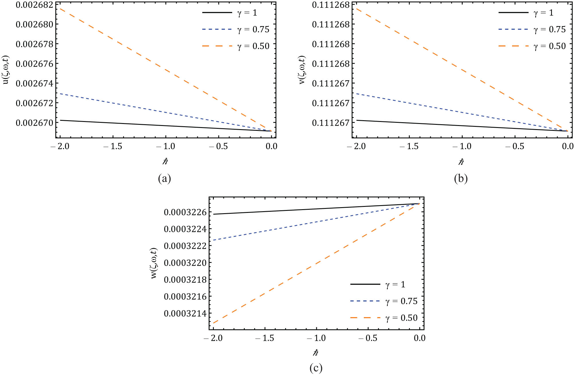
Nature of response of
|
|
Exact solution (
|
MVIM solution (
|
|
Absolute error
|
Absolute error
|
|---|---|---|---|---|---|
|
|
|
|
|
|
|
|
|
|
|
|
|
|
|
|
|
|
|
|
|
|
|
|
|
|
|
|
|
|
|
|
|
|
|
| 00 |
|
|
|
|
|
| 10 |
|
|
|
|
|
| 20 |
|
|
|
|
|
| 30 |
|
|
|
|
|
| 40 |
|
|
|
|
|
| 50 |
|
|
|
|
|
|
|
Exact solution (
|
MVIM solution (
|
|
Absolute error
|
Absolute error
|
|---|---|---|---|---|---|
|
|
0.0884547 | 0.0884547 | 0.0884547 |
|
|
|
|
0.0884658 | 0.0884657 | 0.0884658 |
|
|
|
|
0.088547 | 0.0885466 | 0.088547 |
|
|
|
|
0.0891299 | 0.089127 | 0.0891298 |
|
|
|
|
0.0926659 | 0.0926551 | 0.0926659 |
|
|
| 00 | 0.102828 | 0.102834 | 0.102828 |
|
|
| 10 | 0.109795 | 0.109802 | 0.109795 |
|
|
| 20 | 0.111293 | 0.111295 | 0.111293 |
|
|
| 30 | 0.111512 | 0.111513 | 0.111512 |
|
|
| 40 | 0.111542 | 0.111542 | 0.111542 |
|
|
| 50 | 0.111546 | 0.111546 | 0.111546 |
|
|
|
|
Exact solution (
|
MVIM solution (
|
|
Absolute error
|
Absolute error
|
|---|---|---|---|---|---|
|
|
|
|
|
|
|
|
|
0.000014879 | 0.0000121481 | 0.0000148777 |
|
|
|
|
0.000109176 | 0.0000893157 | 0.00010916 |
|
|
|
|
0.000766334 | 0.0006360573 | 0.000766258 |
|
|
|
|
0.004017011 | 0.0036024380 | 0.00401731 |
|
|
| 00 | 0.006329433 | 0.0061447985 | 0.00632901 |
|
|
| 10 | 0.001888126 | 0.0019107842 | 0.00188816 |
|
|
| 20 | 0.000292663 | 0.0002919665 | 0.000292708 |
|
|
| 30 | 0.000040371 | 0.0000401720 | 0.0000403782 |
|
|
| 40 |
|
|
|
|
|
| 50 |
|
|
|
|
|
6 Conclusion
We have discussed
-
Funding information: The authors state no funding involved.
-
Author contributions: All authors have accepted responsibility for the entire content of this manuscript and approved its submission.
-
Conflict of interest: The authors state no conflict of interest.
-
Data availability statement: Data sharing is not applicable for this manuscript as no datasets were generated or analyzed during the current study.
References
[1] Miller KS, Ross B. An introduction to the fractional calculus and fractional differential equations. New York: John Wiley & Sons, Inc.; 1993. Search in Google Scholar
[2] Podlubny I. Fractional differential equations: an introduction to fractional derivatives, fractional differential equations, to methods of their solution and some of their applications. San Diego, California, USA: Elsevier; 1998. Search in Google Scholar
[3] Caputo M. Elasticita e Dissipazione. Zanichelli, Bologa, Italy, Links. 1969. Search in Google Scholar
[4] Ross B. The development of fractional calculus 1695–1900. Historia Math. 1977;4(1):75–89. 10.1016/0315-0860(77)90039-8Search in Google Scholar
[5] Singh J, Kumar D, Kumar S. A new fractional model of nonlinear shock wave equation arising in flow of gases. Nonl Eng. 2014;3(1):43–50. 10.1515/nleng-2013-0022Search in Google Scholar
[6] Seadawy A. R. Stability analysis for Zakharov-Kuznetsov equation of weakly nonlinear ion-acoustic waves in a plasma. Comput Math Appl. 2014;67(1):172–80. 10.1016/j.camwa.2013.11.001Search in Google Scholar
[7] Saadeh R, Abbes A, Al-Husban A, Ouannas A, Grassi G. The fractional discrete predator-prey model: chaos, control and synchronization. Fract Fract. 2023;7(2):120. 10.3390/fractalfract7020120Search in Google Scholar
[8] Nisar KS, Ciancio A, Ali KK, Osman MS, Cattani C, Baleanu D, et al. On beta-time-fractional biological population model with abundant solitary wave structures. Alexandr Eng J 2022;61(3):1996–2008. Search in Google Scholar
[9] Singh J, Kumar D, Baleanu D. On the analysis of chemical kinetics system pertaining to a fractional derivative with Mittag-Leffler type kernel. Chaos Interdiscipl J Nonl Sci. 2017;27:10. 10.1063/1.4995032. Search in Google Scholar PubMed
[10] Shchigolev VK. Fractional-order derivatives in cosmological models of accelerated expansion. Modern Phys Lett A 2021;36, (14):2130014. 10.1142/S0217732321300147Search in Google Scholar
[11] Chauhan RP, Kumar S, Alkahtani BST, Alzaid SS. A study on fractional order financial model by using Caputo–Fabrizio derivative. Results Phys. 2024;57:107335. 10.1016/j.rinp.2024.107335Search in Google Scholar
[12] Nisar KS, Farman M, Abdel-Aty M, Ravichandran C. A review of fractional order epidemic models for life sciences problems: past, present and future. Alexandr Eng J. 2024;95:283–305. 10.1016/j.aej.2024.03.059Search in Google Scholar
[13] Alderremy AA, Khan H, Shah R, Aly S, Baleanu D. The analytical analysis of time-fractional Fornberg-Whitham equations. Mathematics. 2020;8(6):987. 10.3390/math8060987Search in Google Scholar
[14] Baleanu D, Wu GC, Zeng SD. Chaos analysis and asymptotic stability of generalized Caputo fractional differential equations. Chaos Solitons Fractals. 2017;102:99–105. 10.1016/j.chaos.2017.02.007Search in Google Scholar
[15] Kapoor M, Kour S. An analytical approach for Yang transform on fractional-order heat and wave equation. Phys Scr. 2024;99(3):035222. 10.1088/1402-4896/ad24abSearch in Google Scholar
[16] Archana DK, Prakasha DG, Veeresha P, Nisar KS. An efficient technique for one-dimensional fractional diffusion equation model for cancer tumor. Comput Model Eng Sci 2024;141(2):1347–63. https://doi.org/10.32604/cmes.2024.053916. Search in Google Scholar
[17] Shah NA, Hamed YS, Abualnaja KM, Chung JD, Shah R, Khan AA. Comparative analysis of fractional-order Kaup–Kupershmidt equation within different operators. Symmetry. 2022;14(5):986. 10.3390/sym14050986Search in Google Scholar
[18] Alshammari S, Al-Sawalha MM, Shah R. Approximate analytical methods for a fractional-order nonlinear system of Jaulent-Miodek equation with energy-dependent Schrodinger potential. Fract Fract. 2023;7(2):140. 10.3390/fractalfract7020140Search in Google Scholar
[19] Baleanu D, Caponetto R, Machado JT. Challenges in fractional dynamics and control theory. J Vibrat Control. 2016;22(9):2151–2. 10.1177/1077546315609262Search in Google Scholar
[20] Darshan Kumar CV, Prakasha DG, Veeresha P, Kapoor M. A homotopy-based computational scheme for two-dimensional fractional cable equation. Modern Phys Lett B. 2024;38(32):2450292. 10.1142/S0217984924502920. Search in Google Scholar
[21] Sun H, Zhang Y, Baleanu D, Chen W, Chen Y. A new collection of real world applications of fractional calculus in science and engineering. Commun Nonl Sci Numer Simul. 2018;64:213–31. 10.1016/j.cnsns.2018.04.019Search in Google Scholar
[22] Alshehry AS, Yasmin H, Shah R, Ullah R, Khan A. Fractional-order modeling: Analysis of foam drainage and Fisher’s equations. Open Phys. 2023;21(1):20230115. 10.1515/phys-2023-0115Search in Google Scholar
[23] De Oliveira EC, Tenreiro Machado JA. A review of definitions for fractional derivatives and integral. Math Problems Eng. 2014;2014:1–17. 10.1155/2014/238459Search in Google Scholar
[24] Gao W, Veeresha P, Prakasha DG, Senel B, Baskonus HM. Iterative method applied to the fractional nonlinear systems arising in thermoelasticity with Mittag-Leffler kernel. Fractals. 2020;28(8):2040040. 10.1142/S0218348X2040040XSearch in Google Scholar
[25] Alwehebi F, Hobiny A, Maturi D. Variational iteration method for solving time-fractional burgers equation using Maple. Appl Math. 2023;14(5):336–48. 10.4236/am.2023.145021Search in Google Scholar
[26] Ali KK, Maneea M. Optical solitons using optimal homotopy analysis method for time-fractional (1+1)-dimensional coupled nonlinear Schrodinger equations. Optik. 2023;283:170907. 10.1016/j.ijleo.2023.170907Search in Google Scholar
[27] Ali HM, Nisar KS, Alharbi WR, Zakarya M. Efficient approximate analytical technique to solve nonlinear coupled Jaulent-Miodek system within a time-fractional order. AIMS Math. 2024;9(3):5671–85. 10.3934/math.2024274Search in Google Scholar
[28] Iqbal A, Nawaz R, Ashraf R, Fewster-Young N. Extension of optimal auxiliary function method to nonlinear Sin Gordon partial differential equations. Partial Differ Equ Appl Math. 2024;10:100735. 10.1016/j.padiff.2024.100735Search in Google Scholar
[29] Shah R, Khan H, Farooq U, Baleanu D, Kumam P, Arif M. A new analytical technique to solve system of fractional-order partial differential equations. IEEE Access. 2019;7:150037–50. 10.1109/ACCESS.2019.2946946Search in Google Scholar
[30] Kumar P, Gao W, Veeresha P, Erturk VS, Prakasha DG, Baskonus HM. Solution of a dengue fever model via fractional natural decomposition and modified predictor-corrector methods. Int J Model Simul Scientif Comput. 2024;15(1):2450007. 10.1142/S1793962324500077Search in Google Scholar
[31] Ashraf R, Nawaz R, Alabdali O, Fewster-Young N, Ali AH, Ghanim F, et al. A new hybrid optimal auxiliary function method for approximate solutions of non-linear fractional partial differential equations. Fract Fract. 2023;7(9):673. 10.3390/fractalfract7090673Search in Google Scholar
[32] Alderremy AA, Gomez-Aguilar JF, Sabir Z, Raja MAZ, Aly S. Numerical investigations of the fractional order derivative-based accelerating universe in the modified gravity. Modern Phys Lett A. 2024;39(1):2350180. 10.1142/S0217732323501808. Search in Google Scholar
[33] Chethan HB, Saadeh R, Prakasha DG, Malagi NS, Qazza A, Nagaraja M, et al. An efficient approximate analytical technique for the fractional model describing the solid tumour invasion. Front Phys. 2024;12:1294506. 10.3389/fphy.2024.1294506Search in Google Scholar
[34] Ahmad H, Farooq M, Khan I, Nawaz R, Fewster-Young N, Askar S. Analysis of nonlinear fractional-order Fisher equation using two reliable techniques. Open Phys. 2024;22(1):20230185. 10.1515/phys-2023-0185Search in Google Scholar
[35] Nisar KS, Ciancio A, Ali KK, Osman MS, Cattani C, Baleanu D, et al. On beta-time-fractional biological population model with abundant solitary wave structures. Alexandr Eng J. 2022;61(3):1996–2008. 10.1016/j.aej.2021.06.106Search in Google Scholar
[36] Wu TY, Zhang JE. On modeling nonlinear long waves. in:Mathematics is for solving problems. Philadelphia: Society for Industrial and Applied Mathematics; 1996. p. 233. Search in Google Scholar
[37] Taghizadeh N, Akbari M, Shahidi M Application of reduced differential transform method to the Wu-Zhang equation. Aust J Basic Appl Sci. 2011;5(5):565–71. Search in Google Scholar
[38] Qasim AF, Ali ZY. Application of modified Adomian decomposition method to (2+1)-dimensional non-linear Wu-Zhang system. J Al-Qadisiyah Comput Sci Math. 2018;10(1):40. 10.29304/jqcm.2018.10.1.340Search in Google Scholar
[39] Zayed EM, Rahman HA. On solving the KdV-Burger’s equation and the Wu-Zhang equations using the modified variational iteration method. Int J Nonl Sci Numer Simul. 2009;10(9):1093–104. 10.1515/IJNSNS.2009.10.9.1093Search in Google Scholar
[40] Maaaa ZY. Homotopy perturbation method for the Wu-Zhang equation in fluid dynamics. J Phys Confer Ser IOP Publish. 2008;96(1):012182. 10.1088/1742-6596/96/1/012182Search in Google Scholar
[41] Yang X. Exact solutions of Wu-Zhang equation via complete discrimination system for polynomial method. Modern Phys Lett A. 2023;38(18–19):2350087. 10.1142/S0217732323500876Search in Google Scholar
[42] Awan AU, Tahir M, Rehman HU. On traveling wave solutions: The Wu-Zhang system describing dispersive long waves. Modern Phys Lett B. 2019;33(6):1950059. 10.1142/S0217984919500593Search in Google Scholar
[43] Kaur B, Gupta RK. Time fractional (2+1)-dimensional Wu-Zhang system: Dispersion analysis, similarity reductions, conservation laws, and exact solutions. Comput Math Appl. 2020;79(4):1031–48. 10.1016/j.camwa.2019.08.014Search in Google Scholar
[44] Khater MM, Attia RA, Lu D. Numerical solutions of nonlinear fractional Wu-Zhang system for water surface versus three approximate schemes. J Ocean Eng Sci. 2019;4(2):144–8. 10.1016/j.joes.2019.03.002Search in Google Scholar
[45] Yasmin H, Alderremy AA, Shah R, Hamid Ganie A, Aly S. Iterative solution of the fractional Wu-Zhang equation under Caputo derivative operator. Front Phys. 2024;12:1333990. 10.3389/fphy.2024.1333990Search in Google Scholar
[46] Tariq KU, Khater MM, Younis M. Explicit, periodic and dispersive soliton solutions to the conformable time-fractional Wu-Zhang system. Modern Phys Lett B. 2021;35(24):2150417. 10.1142/S0217984921504170Search in Google Scholar
[47] Shijun L. Homotopy analysis method: a new analytic method for nonlinear problems. Applied Math Mech. 1998;19:957–62. 10.1007/BF02457955Search in Google Scholar
[48] Singh J, Kumar D, Swroop R. Numerical solution of time-and space-fractional coupled Burgers’ equations via homotopy algorithm. Alexandr Eng J. 2016;55(2):1753–63. 10.1016/j.aej.2016.03.028Search in Google Scholar
[49] Veeresha P, Prakasha DG, Qurashi MA, Baleanu D. A reliable technique for fractional modified Boussinesq and approximate long wave equations. Adv Differ Equ. 2019;2019(1):1–23. 10.1186/s13662-019-2185-2Search in Google Scholar
[50] Kumar D, Singh J, Baleanu D. A new analysis for fractional model of regularized long-wave equation arising in ion acoustic plasma waves. Math Meth Appl Sci. 2017;40(15):5642–53. 10.1002/mma.4414Search in Google Scholar
[51] Prakasha DG, Malagi NS, Veeresha P, Prasannakumara BC. An efficient computational technique for time-fractional Kaup–Kupershmidt equation. Numer Meth Partial Differ Equ. 2021;37(2):1299–316. 10.1002/num.22580Search in Google Scholar
© 2025 the author(s), published by De Gruyter
This work is licensed under the Creative Commons Attribution 4.0 International License.
Articles in the same Issue
- Research Articles
- Single-step fabrication of Ag2S/poly-2-mercaptoaniline nanoribbon photocathodes for green hydrogen generation from artificial and natural red-sea water
- Abundant new interaction solutions and nonlinear dynamics for the (3+1)-dimensional Hirota–Satsuma–Ito-like equation
- A novel gold and SiO2 material based planar 5-element high HPBW end-fire antenna array for 300 GHz applications
- Explicit exact solutions and bifurcation analysis for the mZK equation with truncated M-fractional derivatives utilizing two reliable methods
- Optical and laser damage resistance: Role of periodic cylindrical surfaces
- Numerical study of flow and heat transfer in the air-side metal foam partially filled channels of panel-type radiator under forced convection
- Water-based hybrid nanofluid flow containing CNT nanoparticles over an extending surface with velocity slips, thermal convective, and zero-mass flux conditions
- Dynamical wave structures for some diffusion--reaction equations with quadratic and quartic nonlinearities
- Solving an isotropic grey matter tumour model via a heat transfer equation
- Study on the penetration protection of a fiber-reinforced composite structure with CNTs/GFP clip STF/3DKevlar
- Influence of Hall current and acoustic pressure on nanostructured DPL thermoelastic plates under ramp heating in a double-temperature model
- Applications of the Belousov–Zhabotinsky reaction–diffusion system: Analytical and numerical approaches
- AC electroosmotic flow of Maxwell fluid in a pH-regulated parallel-plate silica nanochannel
- Interpreting optical effects with relativistic transformations adopting one-way synchronization to conserve simultaneity and space–time continuity
- Modeling and analysis of quantum communication channel in airborne platforms with boundary layer effects
- Theoretical and numerical investigation of a memristor system with a piecewise memductance under fractal–fractional derivatives
- Tuning the structure and electro-optical properties of α-Cr2O3 films by heat treatment/La doping for optoelectronic applications
- High-speed multi-spectral explosion temperature measurement using golden-section accelerated Pearson correlation algorithm
- Dynamic behavior and modulation instability of the generalized coupled fractional nonlinear Helmholtz equation with cubic–quintic term
- Study on the duration of laser-induced air plasma flash near thin film surface
- Exploring the dynamics of fractional-order nonlinear dispersive wave system through homotopy technique
- The mechanism of carbon monoxide fluorescence inside a femtosecond laser-induced plasma
- Numerical solution of a nonconstant coefficient advection diffusion equation in an irregular domain and analyses of numerical dispersion and dissipation
- Numerical examination of the chemically reactive MHD flow of hybrid nanofluids over a two-dimensional stretching surface with the Cattaneo–Christov model and slip conditions
- Impacts of sinusoidal heat flux and embraced heated rectangular cavity on natural convection within a square enclosure partially filled with porous medium and Casson-hybrid nanofluid
- Stability analysis of unsteady ternary nanofluid flow past a stretching/shrinking wedge
- Solitonic wave solutions of a Hamiltonian nonlinear atom chain model through the Hirota bilinear transformation method
- Bilinear form and soltion solutions for (3+1)-dimensional negative-order KdV-CBS equation
- Solitary chirp pulses and soliton control for variable coefficients cubic–quintic nonlinear Schrödinger equation in nonuniform management system
- Influence of decaying heat source and temperature-dependent thermal conductivity on photo-hydro-elasto semiconductor media
- Dissipative disorder optimization in the radiative thin film flow of partially ionized non-Newtonian hybrid nanofluid with second-order slip condition
- Bifurcation, chaotic behavior, and traveling wave solutions for the fractional (4+1)-dimensional Davey–Stewartson–Kadomtsev–Petviashvili model
- New investigation on soliton solutions of two nonlinear PDEs in mathematical physics with a dynamical property: Bifurcation analysis
- Mathematical analysis of nanoparticle type and volume fraction on heat transfer efficiency of nanofluids
- Creation of single-wing Lorenz-like attractors via a ten-ninths-degree term
- Optical soliton solutions, bifurcation analysis, chaotic behaviors of nonlinear Schrödinger equation and modulation instability in optical fiber
- Chaotic dynamics and some solutions for the (n + 1)-dimensional modified Zakharov–Kuznetsov equation in plasma physics
- Fractal formation and chaotic soliton phenomena in nonlinear conformable Heisenberg ferromagnetic spin chain equation
- Single-step fabrication of Mn(iv) oxide-Mn(ii) sulfide/poly-2-mercaptoaniline porous network nanocomposite for pseudo-supercapacitors and charge storage
- Novel constructed dynamical analytical solutions and conserved quantities of the new (2+1)-dimensional KdV model describing acoustic wave propagation
- Tavis–Cummings model in the presence of a deformed field and time-dependent coupling
- Spinning dynamics of stress-dependent viscosity of generalized Cross-nonlinear materials affected by gravitationally swirling disk
- Design and prediction of high optical density photovoltaic polymers using machine learning-DFT studies
- Robust control and preservation of quantum steering, nonlocality, and coherence in open atomic systems
- Coating thickness and process efficiency of reverse roll coating using a magnetized hybrid nanomaterial flow
- Dynamic analysis, circuit realization, and its synchronization of a new chaotic hyperjerk system
- Decoherence of steerability and coherence dynamics induced by nonlinear qubit–cavity interactions
- Finite element analysis of turbulent thermal enhancement in grooved channels with flat- and plus-shaped fins
- Modulational instability and associated ion-acoustic modulated envelope solitons in a quantum plasma having ion beams
- Statistical inference of constant-stress partially accelerated life tests under type II generalized hybrid censored data from Burr III distribution
- On solutions of the Dirac equation for 1D hydrogenic atoms or ions
- Entropy optimization for chemically reactive magnetized unsteady thin film hybrid nanofluid flow on inclined surface subject to nonlinear mixed convection and variable temperature
- Stability analysis, circuit simulation, and color image encryption of a novel four-dimensional hyperchaotic model with hidden and self-excited attractors
- A high-accuracy exponential time integration scheme for the Darcy–Forchheimer Williamson fluid flow with temperature-dependent conductivity
- Novel analysis of fractional regularized long-wave equation in plasma dynamics
- Development of a photoelectrode based on a bismuth(iii) oxyiodide/intercalated iodide-poly(1H-pyrrole) rough spherical nanocomposite for green hydrogen generation
- Investigation of solar radiation effects on the energy performance of the (Al2O3–CuO–Cu)/H2O ternary nanofluidic system through a convectively heated cylinder
- Quantum resources for a system of two atoms interacting with a deformed field in the presence of intensity-dependent coupling
- Studying bifurcations and chaotic dynamics in the generalized hyperelastic-rod wave equation through Hamiltonian mechanics
- A new numerical technique for the solution of time-fractional nonlinear Klein–Gordon equation involving Atangana–Baleanu derivative using cubic B-spline functions
- Interaction solutions of high-order breathers and lumps for a (3+1)-dimensional conformable fractional potential-YTSF-like model
- Hydraulic fracturing radioactive source tracing technology based on hydraulic fracturing tracing mechanics model
- Numerical solution and stability analysis of non-Newtonian hybrid nanofluid flow subject to exponential heat source/sink over a Riga sheet
- Numerical investigation of mixed convection and viscous dissipation in couple stress nanofluid flow: A merged Adomian decomposition method and Mohand transform
- Effectual quintic B-spline functions for solving the time fractional coupled Boussinesq–Burgers equation arising in shallow water waves
- Analysis of MHD hybrid nanofluid flow over cone and wedge with exponential and thermal heat source and activation energy
- Solitons and travelling waves structure for M-fractional Kairat-II equation using three explicit methods
- Impact of nanoparticle shapes on the heat transfer properties of Cu and CuO nanofluids flowing over a stretching surface with slip effects: A computational study
- Computational simulation of heat transfer and nanofluid flow for two-sided lid-driven square cavity under the influence of magnetic field
- Irreversibility analysis of a bioconvective two-phase nanofluid in a Maxwell (non-Newtonian) flow induced by a rotating disk with thermal radiation
- Hydrodynamic and sensitivity analysis of a polymeric calendering process for non-Newtonian fluids with temperature-dependent viscosity
- Exploring the peakon solitons molecules and solitary wave structure to the nonlinear damped Kortewege–de Vries equation through efficient technique
- Modeling and heat transfer analysis of magnetized hybrid micropolar blood-based nanofluid flow in Darcy–Forchheimer porous stenosis narrow arteries
- Activation energy and cross-diffusion effects on 3D rotating nanofluid flow in a Darcy–Forchheimer porous medium with radiation and convective heating
- Insights into chemical reactions occurring in generalized nanomaterials due to spinning surface with melting constraints
- Influence of a magnetic field on double-porosity photo-thermoelastic materials under Lord–Shulman theory
- Soliton-like solutions for a nonlinear doubly dispersive equation in an elastic Murnaghan's rod via Hirota's bilinear method
- Analytical and numerical investigation of exact wave patterns and chaotic dynamics in the extended improved Boussinesq equation
- Nonclassical correlation dynamics of Heisenberg XYZ states with (x, y)-spin--orbit interaction, x-magnetic field, and intrinsic decoherence effects
- Exact traveling wave and soliton solutions for chemotaxis model and (3+1)-dimensional Boiti–Leon–Manna–Pempinelli equation
- Unveiling the transformative role of samarium in ZnO: Exploring structural and optical modifications for advanced functional applications
- On the derivation of solitary wave solutions for the time-fractional Rosenau equation through two analytical techniques
- Analyzing the role of length and radius of MWCNTs in a nanofluid flow influenced by variable thermal conductivity and viscosity considering Marangoni convection
- Advanced mathematical analysis of heat and mass transfer in oscillatory micropolar bio-nanofluid flows via peristaltic waves and electroosmotic effects
- Exact bound state solutions of the radial Schrödinger equation for the Coulomb potential by conformable Nikiforov–Uvarov approach
- Some anisotropic and perfect fluid plane symmetric solutions of Einstein's field equations using killing symmetries
- Nonlinear dynamics of the dissipative ion-acoustic solitary waves in anisotropic rotating magnetoplasmas
- Curves in multiplicative equiaffine plane
- Exact solution of the three-dimensional (3D) Z2 lattice gauge theory
- Propagation properties of Airyprime pulses in relaxing nonlinear media
- Symbolic computation: Analytical solutions and dynamics of a shallow water wave equation in coastal engineering
- Wave propagation in nonlocal piezo-photo-hygrothermoelastic semiconductors subjected to heat and moisture flux
- Comparative reaction dynamics in rotating nanofluid systems: Quartic and cubic kinetics under MHD influence
- Laplace transform technique and probabilistic analysis-based hypothesis testing in medical and engineering applications
- Physical properties of ternary chloro-perovskites KTCl3 (T = Ge, Al) for optoelectronic applications
- Gravitational length stretching: Curvature-induced modulation of quantum probability densities
- The search for the cosmological cold dark matter axion – A new refined narrow mass window and detection scheme
- A comparative study of quantum resources in bipartite Lipkin–Meshkov–Glick model under DM interaction and Zeeman splitting
- PbO-doped K2O–BaO–Al2O3–B2O3–TeO2-glasses: Mechanical and shielding efficacy
- Nanospherical arsenic(iii) oxoiodide/iodide-intercalated poly(N-methylpyrrole) composite synthesis for broad-spectrum optical detection
- Sine power Burr X distribution with estimation and applications in physics and other fields
- Numerical modeling of enhanced reactive oxygen plasma in pulsed laser deposition of metal oxide thin films
- Dynamical analyses and dispersive soliton solutions to the nonlinear fractional model in stratified fluids
- Computation of exact analytical soliton solutions and their dynamics in advanced optical system
- An innovative approximation concerning the diffusion and electrical conductivity tensor at critical altitudes within the F-region of ionospheric plasma at low latitudes
- An analytical investigation to the (3+1)-dimensional Yu–Toda–Sassa–Fukuyama equation with dynamical analysis: Bifurcation
- Swirling-annular-flow-induced instability of a micro shell considering Knudsen number and viscosity effects
- Numerical analysis of non-similar convection flows of a two-phase nanofluid past a semi-infinite vertical plate with thermal radiation
- MgO NPs reinforced PCL/PVC nanocomposite films with enhanced UV shielding and thermal stability for packaging applications
- Optimal conditions for indoor air purification using non-thermal Corona discharge electrostatic precipitator
- Investigation of thermal conductivity and Raman spectra for HfAlB, TaAlB, and WAlB based on first-principles calculations
- Tunable double plasmon-induced transparency based on monolayer patterned graphene metamaterial
- DSC: depth data quality optimization framework for RGBD camouflaged object detection
- A new family of Poisson-exponential distributions with applications to cancer data and glass fiber reliability
- Numerical investigation of couple stress under slip conditions via modified Adomian decomposition method
- Monitoring plateau lake area changes in Yunnan province, southwestern China using medium-resolution remote sensing imagery: applicability of water indices and environmental dependencies
- Heterodyne interferometric fiber-optic gyroscope
- Exact solutions of Einstein’s field equations via homothetic symmetries of non-static plane symmetric spacetime
- A widespread study of discrete entropic model and its distribution along with fluctuations of energy
- Empirical model integration for accurate charge carrier mobility simulation in silicon MOSFETs
- The influence of scattering correction effect based on optical path distribution on CO2 retrieval
- Anisotropic dissociation and spectral response of 1-Bromo-4-chlorobenzene under static directional electric fields
- Role of tungsten oxide (WO3) on thermal and optical properties of smart polymer composites
- Analysis of iterative deblurring: no explicit noise
- The influence of anisotropy of InP on its elasticity and phonon properties
- Review Article
- Examination of the gamma radiation shielding properties of different clay and sand materials in the Adrar region
- Erratum
- Erratum to “On Soliton structures in optical fiber communications with Kundu–Mukherjee–Naskar model (Open Physics 2021;19:679–682)”
- Special Issue on Fundamental Physics from Atoms to Cosmos - Part II
- Possible explanation for the neutron lifetime puzzle
- Special Issue on Nanomaterial utilization and structural optimization - Part III
- Numerical investigation on fluid-thermal-electric performance of a thermoelectric-integrated helically coiled tube heat exchanger for coal mine air cooling
- Special Issue on Nonlinear Dynamics and Chaos in Physical Systems
- Analysis of the fractional relativistic isothermal gas sphere with application to neutron stars
- Abundant wave symmetries in the (3+1)-dimensional Chafee–Infante equation through the Hirota bilinear transformation technique
- Successive midpoint method for fractional differential equations with nonlocal kernels: Error analysis, stability, and applications
- Novel exact solitons to the fractional modified mixed-Korteweg--de Vries model with a stability analysis