Water-based hybrid nanofluid flow containing CNT nanoparticles over an extending surface with velocity slips, thermal convective, and zero-mass flux conditions

1 Introduction

The mixing of small-sized particles into a base fluid for the purpose of supplementing its thermal features results in a nanofluid. This idea was floated initially by Choi and Eastman [1] for enhancing the thermal conductance of normal fluid. Nanofluid flow is studied for its potential to enhance rates of thermal transference in various applications, including cooling of electronic devices, automotive and industrial heat exchangers, and biomedical applications as noticed by Anjum et al. [2] and Khan et al. [3]. Hybrid nanofluid flow involves two or more dissimilar kinds of nanoparticles distributed in a pure fluid, combining the benefits of different materials to further enrich the thermal features of the fluid. For instance, a hybrid nanofluid might include a mixture of metallic nanoparticles, such as copper, and non-metallic nanoparticles, such as graphene, to exploit the extraordinary thermal features of copper and the excellent mechanical and thermal properties of graphene as noticed by Sriharan et al. [4]. Analytical evaluation of temperature in living tissues is performed by Hobiny et al. [5] using the TPL bio-heat model, supported by experimental verification. Their study focuses on understanding thermal behavior in biological tissues, integrating theory and practical data. The results of their work validate the model’s accuracy in predicting temperature distributions, crucial for medical applications such as hyperthermia therapy and diagnostics. Alzahrani and Abbas [6] evaluated analytically the active living tissues’ thermal damage subject to laser irradiations. The synergy between different nanoparticles can lead to improved thermal conductivity, stability, and thermal flow management in comparison with single-component nanofluids [7]. Ibrahim et al. [8] observed that the flow behavior and heat transference characteristics of hybrid nanofluids are influenced by the connections between the diverse kinds of nanoparticles, their concentration ratios, and the properties of pure liquid. Applications include more efficient cooling systems in electronics, automotive radiators, and advanced thermal management systems in renewable energy technologies [9]. Both nanofluids and hybrid nanofluids significantly impact heat transfer by enhancing the thermal conductance and convective heat transfer coefficients of pure fluid [10]. This leads to improved efficiency in heat exchangers and cooling systems, allowing for more effective thermal management. The increased thermal conductivity and improved convective heat transfer result in reduced energy consumption and better performance in systems ranging from microelectronics cooling to industrial heat exchangers and renewable energy applications. Marin et al. [11] numerically examined a nonlinear hyperbolic bio-thermal model under various flow conditions to treat tumor cells. The study aimed to understand the interaction between heat transfer and biological tissue in the context of tumor treatment. Their findings contribute to optimizing therapeutic strategies, enhancing the understanding of heat-induced cell damage, and improving treatment protocols for tumors. The investigation of Saeed and Abbas [12] focuses on mathematical models of bio-heat transfer to analyze the transient phenomena in spherical tissue caused by a laser heat source. Their study aims to understand how the tissue responds to the heat over time, considering the impact of the laser on the thermal behavior of the biological material. Hobiny and Abbas [13] examined the nonlinear analysis of the dual-phase lag model of bio-heat in living tissues under laser irradiation. Their work focuses on understanding heat transfer dynamics, accounting for time delays in heat flux and temperature gradient responses, and offering insights into thermal behavior during laser–tissue interactions for medical and scientific applications.

Porous media describe the materials containing pores within their structure, which allow fluids (liquids or gases) to pass through. These materials occur naturally, such as soils, rocks, and biological tissues, or engineered, such as ceramics, foams, and certain types of filters. The pores in porous media vary significantly in size, shape, and distribution, influencing the material’s permeability and porosity. Fluid flow in porous media involves the movement of fluids through materials that contain numerous pores or voids and is primarily governed by Darcy’s law as observed by Yang et al. [14]. Khalil et al. [15] proved that in permeable media, the fluid flow is affected by the porosity and the permeability of the material, as well as the viscosity and density of the fluid. Wang et al. [16] studied the mass and thermal transportations of thin-film flow on a permeable medium with impressions of the Buongiorno model. Pop et al. [17] discussed time-based flow and thermal transference for mono and hybrid nanoparticle flow on a permeable surface and noted that with progression in porosity factor, there has been a decline in velocity distribution while a growth has noted thermal distribution. In practical applications, such as groundwater hydrology, oil recovery, and filtration, the performance of fluid flow in porous media is crucial for heightening the efficacy and effectiveness of a process [18]. The motion of fluid on a permeable media significantly affects thermal and velocity panels within the medium as noted by Ali et al. [19]. For the heterogeneous nature of permeable media, the fluid velocity is not uniform and varies with the pore size and distribution. This non-uniformity leads to complex velocity profiles, where fluid may accelerate through larger pores and slowdown in smaller ones, creating a range of velocities within the medium. Temperature profiles in porous media are also impacted by the flow as noted by Nadeem et al. [20], the thermal conductance of the porous medium, combined with the convective heat transfer of the fluid, determines the temperature distribution.

The key principle of MHD is the relationship between the magnetic fields and the fluid’s electrical conductivity, which induces currents and affects the fluid motion. Governed by the combined principles of fluid dynamics and electromagnetism, MHD finds applications in astrophysics, fusion reactors, and electromagnetic pumps [21,22]. Ahmad et al. [23] studied the significance of multi-slip constraints with impacts of MHD on fluid flow subject of nonlinear radiations thermally and chemically reactivity. Lone et al. [24] discussed a semi-numerical approach for the evaluation of blood-based trihybrid MHD fluid flow on a bi-directional extending sheet with flow slip constraints. In MHD, the existence of a magnetic field considerably influences the velocity and thermal distributions of the conducted fluid as observed by Tarakaramu et al. [25]. Mahesh et al. [26] proved that the Lorentz force, resulting from the interaction between the magnetic field and the induced electric current, acts on the fluid, modifying its flow characteristics. In some cases, MHD also induces secondary flows, such as swirling or rotational movements, subject to the alignment and strength of the magnetic field [27]. Moreover, Lund et al. [28] noted that the occurrence of the magnetic field in a fluid alters the heat transfer mechanisms. However, in some scenarios, it also suppresses convective motion, leading to increased reliance on conduction for heat transfer. Furthermore, as studied by Nawaz et al. [29], MHD can be utilized to control and optimize thermal management in various applications, such as cooling systems in fusion reactors or electromagnetic braking in metallurgy. The overall impact on velocity and thermal distributions depends on factors such as magnetic field strength, fluid properties, and flow conditions, making MHD a versatile tool in engineering and scientific research. Hobiny and Abbas [30] examined experimentally the thermal response of cylindrical tissues subject to laser irradiations. Abbas et al. [31] evaluated analytically the model of bio-heat for spherical tissues using the impacts of laser irradiations.

Brownian motion describes the random movement of particles mixed in a fluid, resulting from collisions of the molecules of fluids. This phenomenon is more pronounced at smaller scales, such as nanoparticles, where thermal fluctuations cause significant particle displacement. Brownian motion affects fluid dynamics by enhancing the mixing and dispersion of particles within the fluid as proved by Madkhali et al. [32]. Thermophoresis is the migration of particles in a fluid for thermal gradient in the flow phenomenon. Particles tend to move from hotter to cooler regions, driven by the imbalance in kinetic energy between particles in different thermal zones. Both thermophoresis and Brownian motion considerably affect heat and concentration transfer in fluid systems [33]. Shahzad et al. [34] studied that the Brownian motion enhances thermal conductance by promoting the uniform distribution of nanoparticles, leading to better heat transfer in nanofluids. Thermophoresis, in contrast, creates a thermal gradient-driven particle movement, which either enhances or inhibits heat transfer subject to the direction of the temperature gradient relative to the desired heat flow [35]. Brownian motion increases particle dispersion, improving the mixing and homogeneity of the solute concentration in the fluid. This leads to more efficient mass transfer and reaction rates in processes such as chemical reactions or pollutant dispersion. Sharma et al. [36] proved that thermophoresis effects contribute to concentration gradients by causing particles to migrate toward cooler regions, affecting the local concentration profiles and potentially enhancing separation processes or creating regions of high particle concentration. Thabet et al. [37] studied thermal augmentation for MHD fluid flow with impacts of Brownian and thermophoretic diffusions. Hanı et al. [38] discussed the impacts of Brownian and thermophoretic diffusions on boundary-layer MHD fluid flow on an elongating surface. Waqas et al. [39] examined computationally the Brownian motion and thermophoretic effects on gyrating nanomaterial fluid flow with activation energy.

Thermal radiation is electromagnetic radiation emitted by a body due to its temperature. It encompasses a range of wavelengths, including infrared, visible, and ultraviolet light, with intensity and wavelength distribution dependent on the body’s temperature. Thermal radiation significantly impacts the thermal characteristics distribution within the fluid and the boundaries it interacts with [40]. This combined heat transfer mechanism is essential in high-temperature environments, such as combustion chambers, solar collectors, and industrial furnaces. Essam and Abedel-AaL [41] proved that thermal radiation enhances heat transfer by providing a surplus mode of energy transfer, supplementing conduction and convection. Pandey et al. [42] studied thermally radiative and mixed convective fluid flow on a surface. Gul et al. [43] discussed the thin flow of carbon nanotubes (CNTs) with magnetic effects on a belt and have proved that pressure profiles, velocity, and thermal transmission have affected more in the case of multi-walled carbon nanotubes (MWCNTs). Alrehili [44] inspected augmentation in heat transfer for nanoparticle fluid flow on a nonlinear elongating surface with thermal radiations. Wang et al. [45] proved that in high-temperature applications, radiative heat transfer dominates, leading to more uniform temperature distributions and improved thermal efficiency. The presence of thermal radiation affects the fluid’s temperature gradients, often resulting in increased heat transfer rates as noted by Goud et al. [46]. Muhammad et al. [47] inspected the slip flow of mixed convective mono/hybrid nanofluids on a curved sheet. In their study, the authors have conducted a comparative analysis to ensure the precision of their results established. This is particularly important in systems where maintaining high thermal performance is critical, such as in the thermal management of electronic devices, high-temperature industrial processes, and energy systems such as solar thermal collectors. By optimizing the role of thermal radiation, engineers can design more efficient thermal systems with improved performance and energy savings. Swain et al. [48] studied computationally 3D Maxwell fluid flow on a stretching surface with impacts of thermal radiations. Hamad et al. [49] discussed the third-grade fluid flow on an inclined elongating surface with magnetic and thermally radiative effects. Hayat et al. [50] studied the Eyring Powell fluid flow with impacts of nanoparticles on exponential elongating sheet. In their work, the authors have conducted a comparative investigation to ensure the validity of the method used for the solution.

Single-walled carbon nanotubes (SWCNTs) are geometrical structures in cylindrical form with a single layer of carbon atoms arranged in a hexagonal lattice. SWCNTs have remarkable electrical, thermal, and mechanical properties due to their unique structure, making them highly conductive and strong. They are used in various applications, including electronics, materials science, and nanotechnology. SWCNTs, with their single-layer structure, offer superior thermal conductivity along their length, making them ideal for applications requiring efficient heat dissipation. They can be used in thermal interface materials and as fillers in composite materials to improve thermal management in electronics and other devices. MWCNTs consist of numerous concentric layers of carbon atoms, forming a series of coaxial cylinders around a central hollow core. MWCNTs are less conductive than SWCNTs due to interlayer interactions. They offer greater mechanical strength and are easier to produce in large quantities. MWCNTs find applications in composite materials, conductive films, and additives to enhance the properties of various materials. MWCNTs, while slightly less efficient than SWCNTs due to interlayer phonon scattering, still provide excellent thermal conductivity. Their larger diameter and multiple layers make them robust and suitable for bulk applications. MWCNTs enhance the thermal conductivity of polymers and other matrices when used as fillers, improving the performance of thermal management systems in various industrial applications. Both types of CNTs are critical in developing advanced materials for efficient heat transfer and thermal regulation. The adoption of convective and zero-mass flux conditions in this analysis is motivated by their practical applications. Convective conditions account for heat exchange between fluid and the surrounding medium, which is critical in systems for improved heat transfer, such as solar collectors, heat sinks, and cooling devices for electronics. In this analysis, single and MWCNT hybrid nanofluid flow is examined on a bi-directional extending sheet. Velocity slips, thermal convective, and zero-mass flux conditions are executed to examine the hybrid nanofluid flow. Also, thermal radiation, exponential heat source, Brownian motion, thermophoresis, chemical reaction, and activation energy effects have been used. In this analysis, the authors are encouraged to investigate how the CNT nanoparticles influence the flow behavior of the water-based hybrid nanofluid flow with numerous constraints, such as velocity slips, thermal convective, and zero-mass flux conditions. How do external factors such as exponential heat source, Brownian motion, thermal radiation, and thermophoresis influence the behavior and efficiency of the water-based hybrid nanofluid flow? What are the effects of the chemical reaction and activation energy on the performance of hybrid nanofluid flow? To answer these questions, the mathematical formulation of the proposed problem is presented in Section 2. The numerical solution of the proposed mathematical model is presented in Section 3. Validation of the present model with published results is presented in Section 4. The present results are discussed in Section 5. The final concluding remarks are shown in Section 6.

2 Problem formulation

A three-dimensional flow of hybrid nanofluid containing SWCNT and MWCNT over an extending sheet using porous media is considered. A Cartesian coordinate system with flow components u , v , w along x , y , z directions is chosen to investigate the hybrid nanofluid flow. Moreover, u w ( x ) = a x and v w ( y ) = b y (with a and b as fixed values) are stretching velocities along x- and y-axes. The z-direction is normal to the xy-plane. The conditions of flow slip ( u slip and v slip ) are also executed in this analysis. The magnetic effect with strength B 0 is employed in a perpendicular direction to the flow system. The working fluid temperature is taken as T f such that ( T f > T w ). The free-stream temperature is denoted by T ∞ . The condition of zero-mass flux is applied such that the mass flow at the sheet surface is zero (i.e., C w = 0 ) [51,52,53]. Furthermore, the free-stream concentration is C ∞ . Also, the thermal radiation, Brownian motion, exponential heat source, thermophoresis, chemical reaction, and activation energy are used in this work. Following the aforementioned assumptions, the leading equations can be expressed as follows [54,55] (Figure 1):

With physical conditions at boundaries [54]:

Figure 1

Geometrical view of flow problem.

The velocity slip conditions ( u slip and v slip ) are defined as

where Δ 1 and Δ 2 are the slip constants.

The effective qualities of mono and hybrid nanofluids are enumerated as follows [53,56] (Table 1):

So, Eq. (1) is satisfied identically, and the remaining equations are as follows:

with related conditions at the boundary as

Some emerging factors are encountered in the aforementioned equations that are mathematically described as follows:

The physical description and ranges of these factors are given in Table 2.

The main quantities of interest such as skin friction C f x , Nusselt number Nu x , and Sherwood number Sh x are described as follows:

where

Thus, Eq. (17) reduces as follows:

Above C f x = − Re x C f x , C f y = − Re x C f y , and Nu = Nu x Re x . Furthermore, Re x = u w ( x ) x ν f and Re x = u w ( x ) x ν f are the local Reynolds numbers.

3 Numerical solution

To acquire the numerical solution modeled equations, the bvp4c technique is chosen. This is a powerful technique that can solve highly nonlinear problems. The error tolerance of 10⁻⁶ is demarcated in the present case. To implement this technique, we must moderate the higher-order nonlinear problem to a first-order problem. Therefore, we assume that

with boundary conditions:

where the subscripts INITIAL and FINAL depict the initial as well as boundary conditions respectively.

4 Validation

This section portrays the validation of the current results against the published findings of Hayat et al. [58] and Dawar et al. [54] for variations in ratio, factor ( λ ). The results are compared for a special case of viscous fluid and the effects of magnetic field and porous media are ignored (i.e., M = K = κ 1 = κ 2 = 0 ). Furthermore, the effects of slip conditions are also ignored (i.e., α 1 = α 2 = 0 ). From this analysis, we have confirmed the correctness of the applied method and proposed model by comparing the present and published results (Table 3).

5 Discussion of results

This section deals with the physical explanation of the obtained results. A numerical investigation of the presented model is carried out by using the bvp4c approach. The obtained results are shown in Tables 4 and 5 and Figures 2–19. Table 4 shows the variation in C f x and C f y via M , K , λ , α 1 , and α 2 . The greater M enhances C f x and C f y . The higher magnetic factor upsurges both C f x and C f y (skin friction coefficients) due to the fact that the magnetic field induces the Lorentz forces that play a role against the motion of fluid particles, which results in an increase in wall shear stress. This causes a higher velocity gradient near the stretching surface, thus enhancing C f x and C f y . The greater K enhances C f x and C f y . In the presence of porous media, the hybrid nanofluid flow experiences opposing forces resulting in a greater velocity gradient at the sheet surface. This increasing velocity gradient leads to a higher wall shear stress, thus enhancing C f x as well as C f y . The greater λ enhances C f x and C f y . As the values of λ enhance, the velocity gradients along the x and y-axes also enhance. The enhanced velocity gradients increase the wall shear stresses, thus enhancing C f x as well as C f y . Furthermore, the higher slip factors ( α 1 and α 2 ) reduce and C f y . Where there is slip, the velocity gradients at the wall reduce due to the fact the fluid velocity is non-zero at the boundary-layer region. The hybrid nanofluid flow has a finite velocity relative to the stretching wall, reducing the velocity gradient. Table 5 shows the variation in Nu via M , Rd , Q Exp , and Bi T . The greater M enhances Nu . The higher magnetic field escalates the rate of heat transfer by modifying the velocity distribution through Lorentz force, which makes turbulence in the flow pattern, and as a result, the higher temperature gradient is determined. This effect contributes to a greater thermal flow rate in MHD flows. The greater Rd enhances Nu . Thermal radiation factor plays a vital role in heat transfer rate. The radiation factor upsurges the rate of heat transfer by adding an additional model of heat transfer, which upsurges the thermal flow rate at the sheet’s surface. The greater Q Exp enhances Nu . The exponential thermal source upsurges the rate of thermal flow by producing significant internal heat generation leading to a higher Nusselt number. The greater Bi T enhances Nu . The higher thermal Biot number enhances the heat transfer coefficient, which results in a greater rate of heat transfer. Therefore, the higher Bi T enhances Nu .

Figure 2

Variation in f ′ ( ξ ) via M .

Figure 3

Variation in g ′ ( ξ ) via M .

Figure 4

Variation in f ′ ( ξ ) via K .

Figure 5

Variation in g ′ ( ξ ) via K .

Figure 6

Variation in f ′ ( ξ ) via λ .

Figure 7

Variation in g ′ ( ξ ) via λ .

Figure 8

Variation in f ′ ( ξ ) via α 1 .

Figure 9

Variation in g ′ ( ξ ) via α 2 .

Figure 10

Variation in θ ( ξ ) via Bi T .

Figure 11

Variation in θ ( ξ ) via Nb .

Figure 12

Variation in χ ( ξ ) via Nb .

Figure 13

Variation in θ ( ξ ) via Nt .

Figure 14

Variation in χ ( ξ ) via Nt .

Figure 15

Variation in θ ( ξ ) via Q Exp .

Figure 16

Variation in θ ( ξ ) via Rd .

Figure 17

Variation in χ ( ξ ) via Sc .

Figure 18

Variation in χ ( ξ ) via Kr .

Figure 19

Variation in χ ( ξ ) via E .

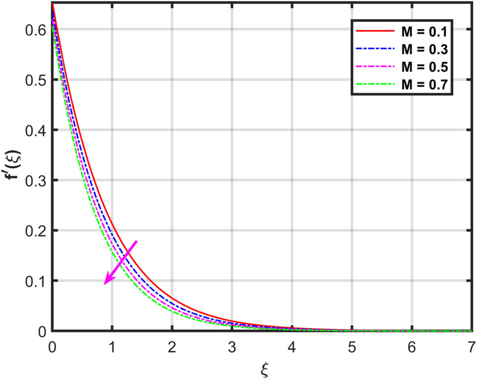
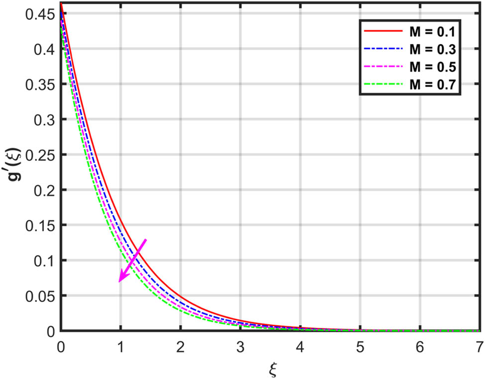
Figures 2 and 3 show the impact of M on f ′ ( ξ ) and g ′ ( ξ ) . From the obtained results, we observed that higher M diminishes both f ′ ( ξ ) and g ′ ( ξ ) . As the magnetic factor enhances, there exists a Lorentz force that resists the flow of electrically conducting hybrid nanofluid when it moves through a magnetic field. Also, the higher Lorentz force reduces the momentum boundary-layer thickness causing a lessening in the velocity profiles of the hybrid nanofluid. Therefore, the greater magnetic factor reduces both f ′ ( ξ ) and g ′ ( ξ ) .

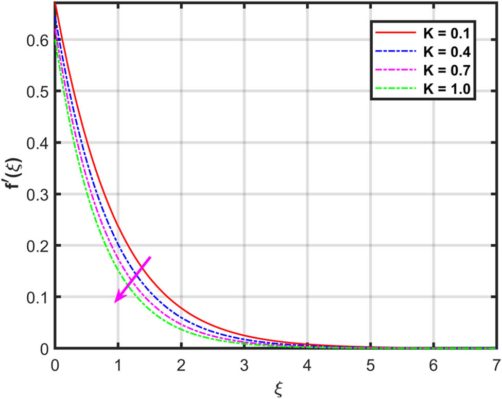
Figures 4 and 5 depict the effects of K on f ′ ( ξ ) and g ′ ( ξ ) . From the obtained results, we perceived that a greater K diminishes both f ′ ( ξ ) and g ′ ( ξ ) . Actually, the greater porosity factor enhances the skin friction coefficients as shown in Table 4. The greater friction force diminishes the momentum boundary-layer width and causes a decline in the velocity profiles in both directions ( f ′ ( ξ ) , g ′ ( ξ ) ). Therefore, the greater porosity factor reduces both f ′ ( ξ ) and g ′ ( ξ ) .

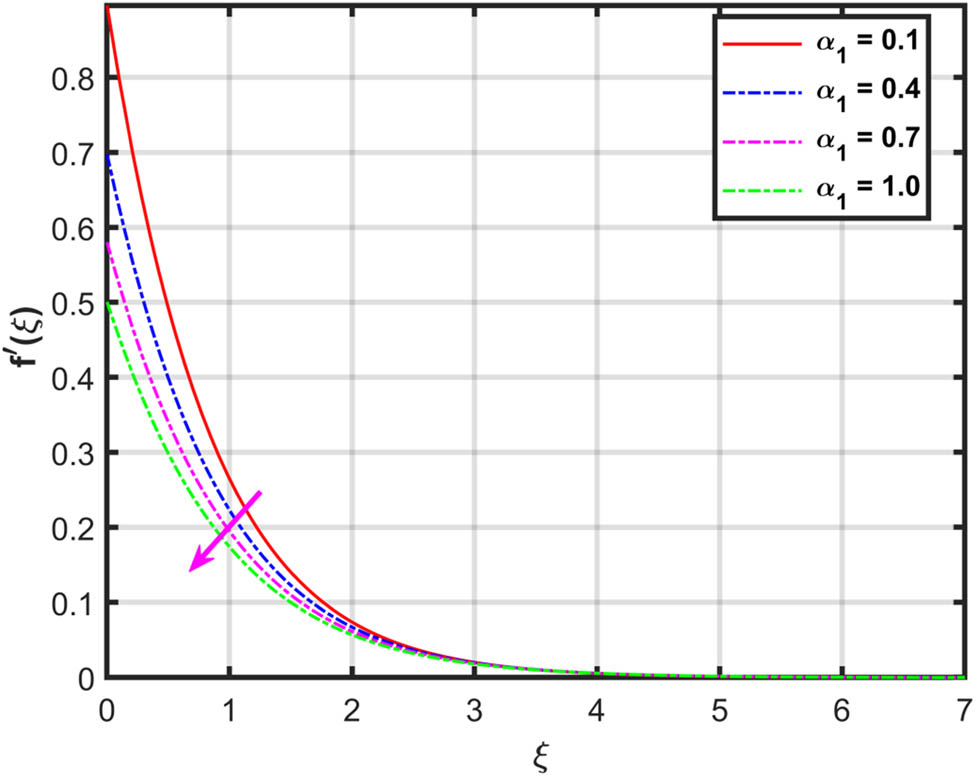
Figures 6 and 7 depict the effects of λ on f ′ ( ξ ) and g ′ ( ξ ) . From the obtained results, we observed that higher values of λ diminishes f ′ ( ξ ) while upsurges g ′ ( ξ ) . By definition, the ratio parameter has a direct relation with the stretching constant of the y-directional velocity ( λ ∝ b ) and inverse relation with the stretching constant of the x-directional velocity ( λ ∝ 1 / a ). As the ratio factor enhances, then the y-directional velocity enhances, which results in higher-velocity profile along the y-direction. In contrast, as the ratio factor enhances, then the x-directional velocity reduces, which results reduction in the velocity profile in the x-direction. Therefore, the higher values of λ reduces f ′ ( ξ ) while increases g ′ ( ξ ) .

Figures 8 and 9, respectively, portray the impressions of the velocity slip parameter α 1 (along the x-axis) on primary velocity f ′ ( ξ ) and velocity slip parameter α 2 (along the y-axis) on secondary velocity g ′ ( ξ ) . As α 1 and α 2 increase along both the coordinates axes, it corresponds to a reduction in f ′ ( ξ ) and g ′ ( ξ ) . This phenomenon is physically observed near the boundary layer of a fluid in contact with a surface where slip conditions hold, like in microfluidics or rarefied gas flows. The velocity slips account for the deviation from the normal no-slip boundary condition, indicating that the fluid velocity at the surface is not zero but rather a fraction of the bulk flow velocity. Consequently, this slip reduces the overall momentum transfer from the fluid to the surface, leading to retardation in the primary and secondary flow velocities. These retardations are critical in applications involving high-precision fluid mechanics, as it impacts the efficiency and performance of fluid systems, necessitating careful consideration in the design and analysis of such systems.

Figure 10 depicts the influences of thermal Biot number Bi T on thermal distribution θ ( ξ ) . Clearly, Bi T is a dimensionless parameter that depicts the ratio of interior heat resistance to the exterior heat resistance between the fluid particles and their surroundings. As Bi T increases, it indicates a higher internal resistance to heat transfer compared to the external resistance. Physically, this means that the temperature gradient in the fluid becomes more significant, causing a more prominent thermal distribution. When Bi T is low, the fluid is assumed to have a nearly uniform temperature, as the external heat transfer dominates. Conversely, as Bi T grows, the internal temperature gradients become more substantial, causing variations in temperature throughout the fluid flow. This augmentation in θ ( ξ ) with increasing Biot number is critical in heat transfer analysis, influencing the design and performance of many thermal systems.

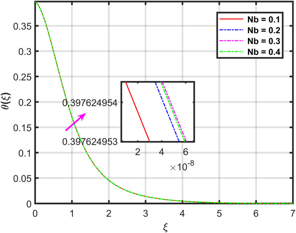
Figure 11 depicts the effects of the Brownian motion factor Nb on thermal panels θ ( ξ ) . As Nb increases, there is a corresponding augmentation in θ ( ξ ) within that fluid. Brownian motion refers to the random, movement of fluid particles suspended in a fluid, resulting from collisions with the fluid’s molecules. Physically, as the intensity of Brownian motion grows, the particles facilitate greater heat transfer through their constant movement, effectively spreading thermal energy more evenly throughout the medium. This phenomenon is particularly significant in nanoscale systems and colloidal suspensions, where particle dynamics play a crucial role in heat conduction. The increased thermal distribution due to enhanced Brownian motion is vital for applications in microfluidics, nanotechnology, and biochemical processes, where precise control over temperature and efficient heat dissipation are essential for optimal performance and reliability.

Figure 12 depicts the influences of Brownian motion factor Nb on χ ( ξ ) .The impact of an upsurge in Nb on χ ( ξ ) exhibits a reducing impact. The concentration distribution is reduced because higher Nb arises from the increased nanoparticles movement within the hybrid nanofluid flow, which results in an enhancement in nanoparticle diffusion. This diffusion of nanoparticles smoothens the concentration gradient by redistributing the nanoparticles more uniformly throughout the hybrid nanofluid. As a result, a higher Nb leads to a reduction in the concentration distribution. Therefore, the higher Nb reduces χ ( ξ ) .

Figure 13 depicts the influences of Nt (thermophoresis factor) on thermal distribution θ ( ξ ) with growth in θ ( ξ ) against variations in Nt . Thermophoresis is actually the motion of particles from zones of higher to lower temperatures due to temperature gradients. When thermophoresis factor Nt increases, the force driving the particle movement becomes stronger. Physically, this enhanced movement contributes to a more effective redistribution of particles, which carry thermal energy across the fluid. As these particles move from hot to cold regions, they facilitate a more uniform temperature distribution by transferring heat. Hence, augmentation in Nt causes the corresponding upsurge in θ ( ξ ) as portrayed in Figure 13.

Figure 14 depicts the influences of Nt on concentration distribution χ ( ξ ) . The impact of an upsurge in Nt on χ ( ξ ) exhibits a twofold behavior, characterized by an initial decline followed by an augmentation. On the interval 0 ≤ ξ < 0.8 , the enhanced movement of particles from hot to cold regions causes a drop in χ ( ξ ) . This occurs because particles are being driven away from the hot regions at the surface of the bi-directional elongating sheet, creating a weakening zone and increasing concentration gradients. However, as Nt continues to rise into the higher range on the interval 0.8 ≤ ξ ≤ 1.0 , the particle movement becomes more prominent, and the particles begin to accumulate in the cooler regions. This accumulation leads to an upsurge in χ ( ξ ) as depicted in Figure 14.

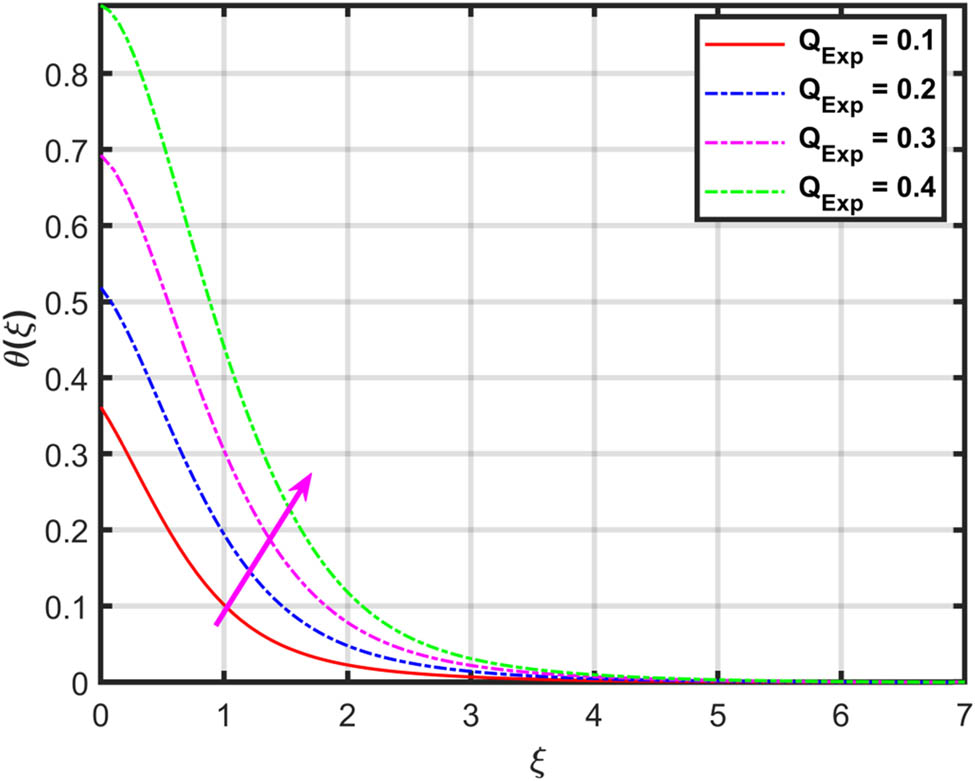
The impact of exponential thermal source factor Q Exp on thermal distribution θ ( ξ ) with augmentation in θ ( ξ ) for variations in Q Exp is depicted in Figure 15. Actually, Q Exp represents a heat source whose intensity increases exponentially. Physically, this means that as the thermal source factor grows, the amount of heat being introduced into the system rises rapidly. This rapid increase in heat input enhances the temperature gradients within the medium, leading to a more extensive thermal distribution. The heat spreads more effectively throughout the fluid, creating broader and more prominent temperature profiles θ ( ξ ) . This phenomenon is particularly important in applications involving laser heating, combustion processes, and nuclear reactions where controlling the distribution of heat is crucial for efficiency and safety. The augmented thermal distribution due to the exponential thermal source factor significantly impacts the thermal management, material properties, and overall performance of various industrial and scientific systems.

The impact of thermal radiation factor Rd on thermal distribution θ ( ξ ) with augmentation in θ ( ξ ) against variations in Rd is depicted in Figure 16. Actually, Rd quantifies the effects of thermal radiation, so as this factor increases, the contribution of radiative heat transfer becomes more significant. Physically, this means that more thermal energy is being radiated and absorbed by the fluid, enhancing the overall heat distribution. The radiative heat transfer is particularly effective over larger distances compared to conduction and convection, allowing for a more uniform temperature spread even in less conductive fluid. Hence, growth in the thermal radiation parameter Rd results in augmentation in thermal distribution θ ( ξ ) as depicted in Figure 16.

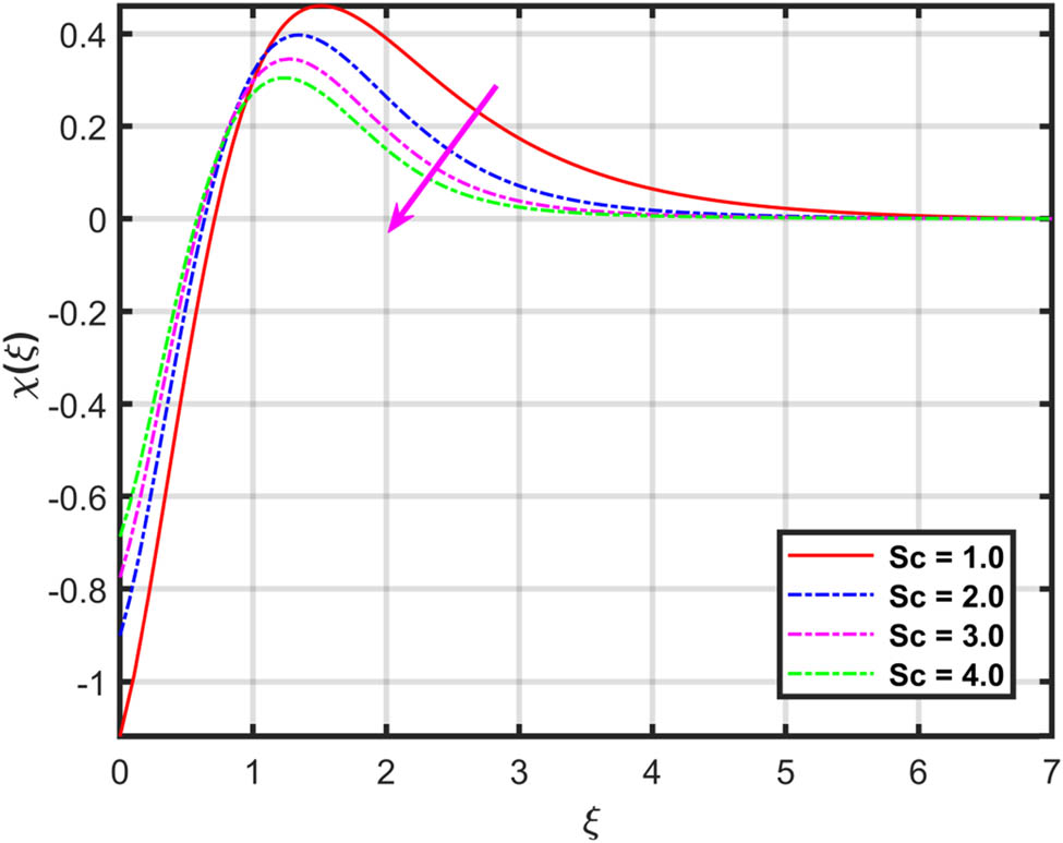
The influence of Schmidt number Sc on χ ( ξ ) is depicted in Figure 17, where growth in Sc has resulted in retardation in χ ( ξ ) . Actually, the Schmidt number Sc describes the ratio of momentum to mass diffusivity. When Sc upsurges, it specifies that the fluid’s viscosity is high relative to its mass diffusivity, meaning that the fluid’s ability to diffuse momentum is much greater than its ability to diffuse mass. Physically, this results in slower mixing and spreading of species within the fluid. In the scenario of fluid flow on the bi-directionally elongating sheet, this high Schmidt number means that the concentration boundary layer becomes thinner, and mass transfer from the sheet into the fluid is less efficient. The fluid’s high viscosity relative to its mass diffusivity inhibits the dispersion of solute particles, leading to the retardation of χ ( ξ ) . This behavior is crucial in applications involving chemical reactions, separation processes, and coating flows, where precise control over mass transfer and concentration profiles is essential for achieving optimal performance and efficiency.

The influence of chemical reactivity parameter Kr on concentration distribution χ ( ξ ) is depicted in Figure 18, where progression in Kr is resulted in hindrance in χ ( ξ ) . The chemical reactivity factor Kr quantifies the rate at which a chemical species reacts within the fluid. As Kr increases, the rate of reaction becomes faster. Physically, this means that the reactive species are consumed more quickly near the surface of the elongating sheet, reducing their concentration in that region. This rapid consumption creates steep concentration gradients and hinders the spread of the species throughout the fluid. Consequently, χ ( ξ ) becomes more localized and less uniform. In the case of fluid flow on the bi-directionally elongating sheet, the elongation tends to stretch and thin the boundary layer, but the high reactivity exacerbates the reduction of reactants near the surface, leading to further retardation in their distribution. This phenomenon is significant in industrial processes involving catalysis, coating technologies, and material synthesis, where controlling the concentration profiles and reaction rates is essential for optimizing efficiency, product quality, and process stability.

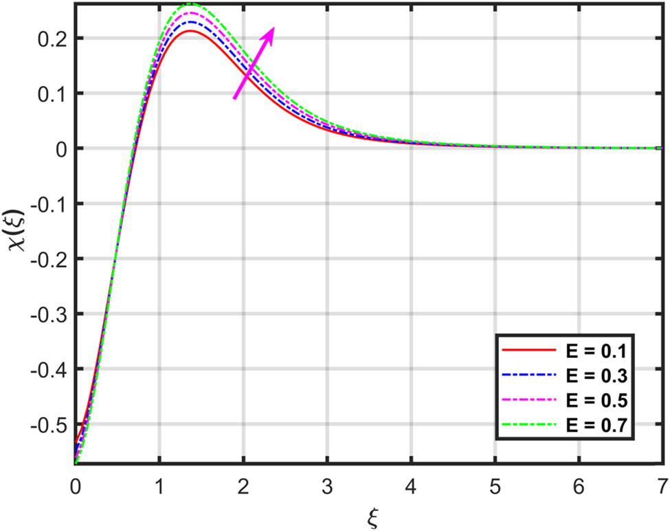
The impacts of activation energy factor E on concentration distribution χ ( ξ ) are depicted in Figure 19, where progression in E has resulted in expansion in χ ( ξ ) . Actually, E characterizes the energy barrier that reactant molecules must overcome to undergo a chemical reaction. As E increases, the activation energy barrier becomes higher, meaning that fewer molecules possess the necessary energy to react. Physically, this leads to a reduction in the rate of chemical reactions near the surface of the elongating sheet, allowing reactants to accumulate more readily in that region. The higher E effectively hinders the alteration of reactants into products, causing an augmentation in their concentration distribution near the sheet’s surface. In the case of fluid flow on bi-directionally elongating sheets, this phenomenon is particularly prominent due to the stretching and thinning of the boundary layer, which enhances the accumulation of reactants. Therefore, growth in E is responsible for augmentation in χ ( ξ ) as portrayed in Figure 19.

6 Conclusions

This work investigates computationally the water-based hybrid nanofluid flow with impacts of CNTs on an elongating surface. The flow is influenced by velocity slip constraints, zero-mass flux conditions, and thermal convection. A magnetic field of specific strength is applied to the flow system in the normal direction. The activation energy and chemical reactivity effects have been used in the concentration equation. The modeled equations have been evaluated numerically through the bvp4c technique after conversion to dimensionless form through the similarity transformation approach. The novelty of this analysis lies in a comprehensive investigation of hybrid nanofluid flow containing CNTs, incorporating velocity slips, and thermal convective and zero-mass flux conditions. The bvp4c solver ensures higher accuracy and consistency in solving the BVPs, with validation achieved through a comparative analysis presenting a robust agreement with the existing studies. A detailed investigation of the work has revealed that:

• With an upsurge in magnetic and porosity factors, the velocities profiles are declined.

• Augmentation in ratio factor has declined the primary velocity profile while supported by the secondary velocity profile.

• Higher values of velocity slip factor along x- and y-axes have retarded both the primary and secondary velocities.

• Thermal distribution has intensified with progression in Brownian motion factor, thermal Biot number thermophoresis factor, and exponential heat source and radiation factors.

• Concentration distribution has escalated with the activation energy factor and has declined with the upsurge in Schmidt number and chemical reactivity factor.

• The impact of an upsurge in the thermophoresis factor enhanced the concentration distribution, while the upsurge in the Brownian motion factor reduced the concentration distribution.

• To ensure the validation of current work, a comparative study has been conducted in this work with a fine agreement among the current and established datasets.

• Growth in magnetic, ratio, and porosity factors cause augmentation in the skin frictions along primary and secondary directions.

References

[1] Choi SU, Eastman JA. Enhancing thermal conductivity of fluids with nanoparticles. 1995 International Mechanical Engineering Congress and Exhibition, San Francisco, CA (United States), 12–17 Nov 1995; Nov 1995;1995.Search in Google Scholar
[2] Anjum N, Khan WA, Azam M, Ali M, Waqas M, Hussain I. Significance of bioconvection analysis for thermally stratified 3D Cross nanofluid flow with gyrotactic microorganisms and activation energy aspects. Therm Sci Eng Prog. 2023;38:101596.10.1016/j.tsep.2022.101596Search in Google Scholar
[3] Khan A, Alyami MA, Alghamdi W, Alqarni MM, Yassen MF, Tag Eldin E. Thermal examination for the micropolar gold–blood nanofluid flow through a permeable channel subject to gyrotactic microorganisms. Front Energy Res. 2022;10:993247.10.3389/fenrg.2022.993247Search in Google Scholar
[4] Sriharan G, Harikrishnan S, Oztop HF. A review on thermophysical properties, preparation, and heat transfer enhancement of conventional and hybrid nanofluids utilized in micro and mini channel heat sink. Sustain Energy Technol Assess. 2023;58:103327.10.1016/j.seta.2023.103327Search in Google Scholar
[5] Hobiny A, Alzahrani F, Abbas I. Analytical estimation of temperature in living tissues using the TPL bioheat model with experimental verification. Mathematics. 2020;8:1188.10.3390/math8071188Search in Google Scholar
[6] Alzahrani FS, Abbas IA. Analytical solutions of thermal damage in living tissues due to laser irradiation. Waves Random Complex Media. 2021;31:1443–56.10.1080/17455030.2019.1676934Search in Google Scholar
[7] Hussain M, Sheremet M. Convection analysis of the radiative nanofluid flow through porous media over a stretching surface with inclined magnetic field. Int Commun Heat Mass Transf. 2023;140:106559.10.1016/j.icheatmasstransfer.2022.106559Search in Google Scholar
[8] Ibrahim IU, Sharifpur M, Meyer JP, Murshed SMS. Experimental investigations of effects of nanoparticle size on force convective heat transfer characteristics of Al2O3-MWCNT hybrid nanofluids in transitional flow regime. Int J Heat Mass Transf. 2024;228:125597.10.1016/j.ijheatmasstransfer.2024.125597Search in Google Scholar
[9] Alrabaiah H, Iftikhar S, Saeed A, Bilal M, Eldin SM, Galal AM. Numerical calculation of Darcy Forchheimer radiative hybrid nanofluid flow across a curved slippery surface. South Afr J Chem Eng. 2023;45:172–81.10.1016/j.sajce.2023.05.013Search in Google Scholar
[10] Yaseen M, Rawat SK, Shah NA, Kumar M, Eldin SM. Ternary hybrid nanofluid flow containing gyrotactic microorganisms over three different geometries with Cattaneo–Christov model. Mathematics. 2023;11:1237.10.3390/math11051237Search in Google Scholar
[11] Marin M, Hobiny A, Abbas I. Finite element analysis of nonlinear bioheat model in skin tissue due to external thermal sources. Mathematics. 2021;9:1459.10.3390/math9131459Search in Google Scholar
[12] Saeed T, Abbas I. Finite element analyses of nonlinear DPL bioheat model in spherical tissues using experimental data. Mech Based Des Struct Mach. 2022;50:1287–97.10.1080/15397734.2020.1749068Search in Google Scholar
[13] Hobiny AD, Abbas IA. Nonlinear analysis of dual-phase lag bio-heat model in living tissues induced by laser irradiation. J Therm Stress. 2020;43:503–11.10.1080/01495739.2020.1722050Search in Google Scholar
[14] Yang Y, Horne RN, Cai J, Yao J. Recent advances on fluid flow in porous media using digital core analysis technology. Adv Geo-Energy Res. 2023;9.10.46690/ager.2023.08.01Search in Google Scholar
[15] Khalil S, Yasmin H, Abbas T, Muhammad T. Analysis of thermal conductivity variation in magneto-hybrid nanofluids flow through porous medium with variable viscosity and slip boundary. Case Stud Therm Eng. 2024;57:104314.10.1016/j.csite.2024.104314Search in Google Scholar
[16] Wang F, Saeed AM, Puneeth V, Shah NA, Anwar MS, Geudri K, et al. Heat and mass transfer of Ag–H2O nano-thin film flowing over a porous medium: A modified Buongiorno’s model. Chin J Phys. 2023;84:330–42.10.1016/j.cjph.2023.01.001Search in Google Scholar
[17] Pop I, Groșan T, Revnic C, Roșca AV. Unsteady flow and heat transfer of nanofluids, hybrid nanofluids, micropolar fluids and porous media: a review. Therm Sci Eng Prog. 2023;46:102248.10.1016/j.tsep.2023.102248Search in Google Scholar
[18] Shu X, Wu Y, Zhang X, Yu F. Experiments and models for contaminant transport in unsaturated and saturated porous media–A review. Chem Eng Res Des. 2023;192:606–21.10.1016/j.cherd.2023.02.022Search in Google Scholar
[19] Ali F, Mahnashi AM, Hamali W, Raizah Z, Saeed A, Khan A. Numerical scrutinization of Darcy–Forchheimer flow for trihybrid nanofluid comprising of $${\text {GO}} + {\text {ZrO}} _ {2} + {\text {SiO}} _ {2} $$/kerosene oil over the curved surface. J Therm Anal Calorim. 2024;1–16.10.1007/s10973-024-13103-wSearch in Google Scholar
[20] Nadeem S, Mushtaq A, Alzabut J, Ghazwani HA, Eldin SM. The flow of an Eyring Powell Nanofluid in a porous peristaltic channel through a porous medium. Sci Rep. 2023;13:9694.10.1038/s41598-023-36136-xSearch in Google Scholar PubMed PubMed Central
[21] Reddy YD, Goud BS, Nisar KS, Alshahrani B, Mahmoud M, Park C. Heat absorption/generation effect on MHD heat transfer fluid flow along a stretching cylinder with a porous medium. Alex Eng J. 2023;64:659–66.10.1016/j.aej.2022.08.049Search in Google Scholar
[22] Mirzaei A, Jalili P, Afifi MD, Jalili B, Ganji DD. Convection heat transfer of MHD fluid flow in the circular cavity with various obstacles: Finite element approach. Int J Thermofluids. 2023;20:100522.10.1016/j.ijft.2023.100522Search in Google Scholar
[23] Ahmad B, Ahmad MO, Farman M, Akgül A, Riaz MB. A significance of multi slip condition for inclined MHD nano-fluid flow with non linear thermal radiations, Dufuor and Sorrot, and chemically reactive bio-convection effect. South Afr J Chem Eng. 2023;43:135–45.10.1016/j.sajce.2022.10.009Search in Google Scholar
[24] Lone SA, Khan A, Raiza Z, Alrabaiah H, Shahab S, Saeed A, et al. A semi-analytical solution of the magnetohydrodynamic blood-based ternary hybrid nanofluid flow over a convectively heated bidirectional stretching surface under velocity slip conditions. AIP Adv. 2024;14.10.1063/5.0201663Search in Google Scholar
[25] Tarakaramu N, Satya Narayana PV, Sivakumar N, Harish Babu D, Bhagya Lakshmi K. Convective conditions on 3D Magnetohydrodynamic (MHD) non-newtonian nanofluid flow with nonlinear thermal radiation and heat absorption: A numerical analysis. J Nanofluids. 2023;12:448–57.10.1166/jon.2023.1939Search in Google Scholar
[26] Mahesh R, Mahabaleshwar US, Kumar PNV, Öztop HF, Abu-Hamdeh N. Impact of radiation on the MHD couple stress hybrid nanofluid flow over a porous sheet with viscous dissipation. Results Eng. 2023;17:100905.10.1016/j.rineng.2023.100905Search in Google Scholar
[27] Ahmad S, Ali K, Sajid T, Bashir U, Rashid FL, Kumar R, et al. A novel vortex dynamics for micropolar fluid flow in a lid-driven cavity with magnetic field localization–A computational approach. Ain Shams Eng J. 2024;15:102448.10.1016/j.asej.2023.102448Search in Google Scholar
[28] Lund LA, Yashkun U, Shah NA. Magnetohydrodynamics streamwise and cross flow of hybrid nanofluid along the viscous dissipation effect: Duality and stability. Phys Fluids. 2023;35.10.1063/5.0135361Search in Google Scholar
[29] Nawaz Y, Arif MS, Abodayeh K, Mansoor M. Finite difference schemes for MHD mixed convective Darcy–forchheimer flow of Non-Newtonian fluid over oscillatory sheet: A computational study. Front Phys. 2023;11:1072296.10.3389/fphy.2023.1072296Search in Google Scholar
[30] Hobiny A, Abbas I. Thermal response of cylindrical tissue induced by laser irradiation with experimental study. Int J Numer Methods Heat Fluid Flow. 2020;30:4013–23.10.1108/HFF-10-2019-0777Search in Google Scholar
[31] Abbas I, Hobiny A, Alzahrani F. An analytical solution of the bioheat model in a spherical tissue due to laser irradiation. Indian J Phys. 2020;94:1329–34.10.1007/s12648-019-01581-wSearch in Google Scholar
[32] Madkhali HA, Ahmed M, Nawaz M, Alharbi SO, Alqahtani AS, Malik MY. Computational study on the effects of Brownian motion and thermophoresis on thermal performance of cross fluid with nanoparticles in the presence of Ohmic and viscous dissipation in chemically reacting regime. Comput Part Mech. 2023;1–11. 10.1007/S40571-023-00687-7/METRICS.Search in Google Scholar
[33] Sudarmozhi K, Iranian D, Alessa N. Investigation of melting heat effect on fluid flow with brownian motion/thermophoresis effects in the occurrence of energy on a stretching sheet. Alex Eng J. 2024;94:366–76.10.1016/j.aej.2024.03.065Search in Google Scholar
[34] Shahzad A, Imran M, Tahir M, Ali Khan S, Akgül A, Abdullaev S, et al. Brownian motion and thermophoretic diffusion impact on Darcy-Forchheimer flow of bioconvective micropolar nanofluid between double disks with Cattaneo-Christov heat flux. Alex Eng J. 2023;62:1–15. 10.1016/J.AEJ.2022.07.023.Search in Google Scholar
[35] Huang Y, Wu C, Dai J, Liu B, Cheng X, Li X, et al. Tunable self-thermophoretic nanomotors with polymeric coating. J Am Chem Soc. 2023;145:19945–52.10.1021/jacs.3c06322Search in Google Scholar PubMed
[36] Sharma BK, Khanduri U, Mishra NK, Mekheimer KS. Combined effect of thermophoresis and Brownian motion on MHD mixed convective flow over an inclined stretching surface with radiation and chemical reaction. Int J Mod Phys B. 2023;37:2350095.10.1142/S0217979223500959Search in Google Scholar
[37] Thabet EN, Khan Z, Abd-Alla AM, Bayones FS. Thermal enhancement, thermophoretic diffusion, and Brownian motion impacts on MHD micropolar nanofluid over an inclined surface: numerical simulation. Numer Heat Transf Part A Appl. 2023;1–20.10.1080/10407782.2023.2276319Search in Google Scholar
[38] Hanı U, Alı M, Alam MS. MHD boundary layer micropolar fluid flow over a stretching wedge surface: Thermophoresis and brownian motion effect. J Therm Eng. 2024;10:330–49.10.18186/thermal.1448609Search in Google Scholar
[39] Waqas H, Khan SA, Ali B, Liu D, Muhammad T, Hou E. Numerical computation of Brownian motion and thermophoresis effects on rotational micropolar nanomaterials with activation energy. Propuls Power Res. 2023.10.1016/j.jppr.2023.05.005Search in Google Scholar
[40] Shah SA, Hassan A, Karamti H, Alhushaybari A, Eldin SM, Galal AM. Effect of thermal radiation on convective heat transfer in MHD boundary layer Carreau fluid with chemical reaction. Sci Rep. 2023;13:4117.10.1038/s41598-023-31151-4Search in Google Scholar PubMed PubMed Central
[41] Essam ME, Abedel-AaL EM. Darcy-forchheimer flow of a nanofluid over a porous plate with thermal radiation and Brownian motion. J Nanofluids. 2023;12:55–64.10.1166/jon.2023.1910Search in Google Scholar
[42] Pandey AK, Bhattacharyya K, Gautam AK, Rajput S, Mandal MS, Chamkha AJ, et al. Insight into the relationship between non-linear mixed convection and thermal radiation: The case of Newtonian fluid flow due to non-linear stretching. Propuls Power Res. 2023;12:153–65.10.1016/j.jppr.2022.11.002Search in Google Scholar
[43] Gul T, Bilal M, Shuaib M, Mukhtar S, Thounthong P. Thin film flow of the water‐based carbon nanotubes hybrid nanofluid under the magnetic effects. Heat Transf. 2020;49:3211–27.10.1002/htj.21770Search in Google Scholar
[44] Alrehili M. Improvement for engineering applications through a dissipative Carreau nanofluid fluid flow due to a nonlinearly stretching sheet with thermal radiation. Case Stud Therm Eng. 2023;42:102768.10.1016/j.csite.2023.102768Search in Google Scholar
[45] Wang X, Shan S, Zhang B, Jin G, Yu J, Zhou Z. Parametrical study on spectral radiation characteristics of solid fuel combustion medium for energy cascade utilization. Fuel. 2024;361:130660.10.1016/j.fuel.2023.130660Search in Google Scholar
[46] Goud BS, Srilatha P, Mahendar D, Srinivasulu T, Reddy YD. Thermal radiation effect on thermostatically stratified MHD fluid flow through an accelerated vertical porous plate with viscous dissipation impact. Partial Differ Equ Appl Math. 2023;7:100488.10.1016/j.padiff.2023.100488Search in Google Scholar
[47] Muhammad K, Hayat T, Alsaedi A, Ahmad B, Momani S. Mixed convective slip flow of hybrid nanofluid (MWCNTs + Cu + Water), nanofluid (MWCNTs + Water) and base fluid (Water): a comparative investigation. J Therm Anal Calorim. 2021;143:1523–36.10.1007/s10973-020-09577-zSearch in Google Scholar
[48] Swain K, Ibrahim SM, Dharmaiah G, Noeiaghdam S. Numerical study of nanoparticles aggregation on radiative 3D flow of Maxwell fluid over a permeable stretching surface with thermal radiation and heat source/sink. Results Eng. 2023;19:101208.10.1016/j.rineng.2023.101208Search in Google Scholar
[49] Hamad NH, Bilal M, Ali A, Eldin SM, Sharaf M, Rahman MU. Energy transfer through third‐grade fluid flow across an inclined stretching sheet subject to thermal radiation and Lorentz force. Sci Rep. 2023;13:19643.10.1038/s41598-023-46428-xSearch in Google Scholar PubMed PubMed Central
[50] Hayat T, Ashraf B, Shehzad SA, Abouelmagd E. Three-dimensional flow of Eyring Powell nanofluid over an exponentially stretching sheet. Int J Numer Methods Heat Fluid Flow. 2015;25:593–616.10.1108/HFF-05-2014-0118Search in Google Scholar
[51] Sun X, Animasaun IL, Swain K, Shah NA, Wakif A, Olanrewaju PO. Significance of nanoparticle radius, inter‐particle spacing, inclined magnetic field, and space‐dependent internal heating: The case of chemically reactive water conveying copper nanoparticles. ZAMM‐J Appl Math Mech Für Angew Math Und Mech. 2022;102:e202100094.10.1002/zamm.202100094Search in Google Scholar
[52] Upadhya SM, Raju SSK, Raju CSK, Mnasri C. Arrhenius activation and zero mass flux conditions on nonlinear convective Jeffrey fluid over an electrically conducting and radiated sheet. Arab J Sci Eng. 2020;45:9095–109.10.1007/s13369-020-04687-0Search in Google Scholar
[53] Dawar A, Islam S, Shah Z, Mahmuod SR. A passive control of Casson hybrid nanofluid flow over a curved surface with alumina and copper nanomaterials: a study on sodium alginate-based fluid. J Mol Liq. 2023;122018.10.1016/j.molliq.2023.122018Search in Google Scholar
[54] Dawar A, Wakif A, Saeed A, Shah Z, Muhammad T, Kumam P. Significance of Lorentz forces on Jeffrey nanofluid flows over a convectively heated flat surface featured by multiple velocity slips and dual stretching constraint: a homotopy analysis approach. J Comput Des Eng. 2022;9:564–82.10.1093/jcde/qwac019Search in Google Scholar
[55] Waqas H, Farooq U, Alqarni MS, Muhammad T. Numerical investigation for 3D bioconvection flow of Carreau nanofluid with heat source/sink and motile microorganisms. Alex Eng J. 2022;61:2366–75.10.1016/j.aej.2021.06.089Search in Google Scholar
[56] Acharya N, Mabood F. On the hydrothermal features of radiative Fe3O4–graphene hybrid nanofluid flow over a slippery bended surface with heat source/sink. J Therm Anal Calorim. 2021;143:1273–89. 10.1007/S10973-020-09850-1/METRICS.Search in Google Scholar
[57] Kumar TP. Heat transfer of SWCNT-MWCNT based hybrid nanofluid boundary layer flow with modified thermal conductivity model. J Adv Res Fluid Mech Therm Sci. 2022;92:13–24.10.37934/arfmts.92.2.1324Search in Google Scholar
[58] Hayat T, Awais M, Obaidat S. Three-dimensional flow of a Jeffery fluid over a linearly stretching sheet. Commun Nonlinear Sci Numer Simul. 2012;17:699–707.10.1016/j.cnsns.2011.05.042Search in Google Scholar
© 2025 the author(s), published by De Gruyter
This work is licensed under the Creative Commons Attribution 4.0 International License.
Articles in the same Issue
- Research Articles
- Single-step fabrication of Ag2S/poly-2-mercaptoaniline nanoribbon photocathodes for green hydrogen generation from artificial and natural red-sea water
- Abundant new interaction solutions and nonlinear dynamics for the (3+1)-dimensional Hirota–Satsuma–Ito-like equation
- A novel gold and SiO2 material based planar 5-element high HPBW end-fire antenna array for 300 GHz applications
- Explicit exact solutions and bifurcation analysis for the mZK equation with truncated M-fractional derivatives utilizing two reliable methods
- Optical and laser damage resistance: Role of periodic cylindrical surfaces
- Numerical study of flow and heat transfer in the air-side metal foam partially filled channels of panel-type radiator under forced convection