Symbolic computation: Analytical solutions and dynamics of a shallow water wave equation in coastal engineering

Qing Chen; Wen-Hui Zhu

doi:10.1515/phys-2025-0223

Article Open Access

Symbolic computation: Analytical solutions and dynamics of a shallow water wave equation in coastal engineering

Qing Chen and Wen-Hui Zhu

Published/Copyright: October 25, 2025

Published by

Become an author with De Gruyter Brill

Submit Manuscript Author Information Explore this Subject

From the journal Open Physics Volume 23 Issue 1

Abstract

This study investigates a shallow water wave-like scalar equation relevant to coastal engineering, employing an innovative computational framework and Mathematica software to derive the analytical solutions. Rational solutions are constructed by using polynomial expansions about x and t . Furthermore, double-periodic soliton solutions are obtained through direct functional Ansätz techniques, while hyperbolic-type and trigonometric-type localized wave solutions are derived by using an improved ( G ′ ∕ G ) -expansion method. In addition to these solutions, we also provided the corresponding Mathematica software calculation code. The dynamic behaviors of these solutions including amplitude modulation, phase interactions, and waveform stability are analyzed and visualized via three-dimensional map and contour map. This study connects theoretical progress in integrable systems with real-world uses in modeling coastal water dynamics.

Keywords: mathematica software; (G’/G)-expansion method; symbolic computation; dynamic properties

1 Introduction

Nonlinear partial differential equations (NLPDEs) are powerful tools in modern science, helping us model complex systems like ocean waves, light pulses in fiber optics, and quantum interactions [1–6]. Finding exact solutions to these equations remains a key challenge with both theoretical and practical importance.

In the 1950s, a major breakthrough occurred with the discovery of solitons, which are stable wave packets that maintain their shape while moving. This discovery has sparked widespread interest in NLPDEs and their solutions [7–11]. Over time, researchers have developed various methods to solve these equations, including Darboux transformation [12,13], Riemann–Hilbert method [14], ( G ′ ∕ G ) -expansion method [15], Kudryashov-expansion method [16], long wave limit method [17], Hirota’s method [18], and Positive quadratic function method [19,20].

In this article, under investigation is the following shallow water wave-like scalar equation [21]

(1) 1 2 u t u 2 + 3 2 u x t u + u t − 3 2 u t u x + u x = 0 ,

where u = u ( x , t ) . Hu et al. [21] have found breather and lump-periodic wave solutions for Eq. (1). The shallow water wave equation is a type of partial differential equation that describes fluid flow under pressure. When the horizontal distance is much greater than the vertical distance, we can obtain the shallow water wave equation by integrating the Navier–Stokes equation over depth. Because of the conservation of mass, the fluid’s vertical movement is not as important as its horizontal movement. The momentum equation tells us that the vertical pressure change is due to the fluid’s weight, while the horizontal pressure change is caused by the movement of the pressure measuring point. This means that the horizontal speed stays the same at all depths in the fluid, as explained in the study by Tukur et al. [21].

The structure of this work is organized as follows: Section 2 derives rational solutions through the polynomial function method [22] and provides the corresponding Mathematica software code. Section 3 presents some double periodic soliton solutions by a direct assumption and gives the corresponding Mathematica software code. In Section 4, we employ an improved ( G ′ ∕ G ) -expansion method to investigate both hyperbolic-type and trigonometric-type solutions. The corresponding Mathematica software code is also presented. Section 5 examines the dynamic characteristics of these obtained solutions by using 3D and contour maps. Finally, Section 6 provides a conclusion.

2 Rational solutions

Making the following transformation based on the Hirota bilinear method

(2) u = 3 ( ln ϑ ) x , ϑ = ϑ ( x , t ) .

Eq. (1) is transformed into

(3) − 9 ϑ x t ϑ x x + 2 ϑ ( ϑ x t + ϑ x x ) + ϑ x [ 9 ϑ x x t − 2 ( ϑ t + ϑ x ) ] = 0 .

Aiming to find the rational solutions for Eq. (1), we suppose

(4) ϑ = ∑ i = 0 2 ∑ j = 0 2 τ i , j x i t j ,

where τ i , j ( i = 0 , 1, 2; j = 0 , 1, 2) are unknown constants. Substituting Eq. (4) in Eq. (3), we obtain

(5) τ 0,0 = τ 1,0 ( τ 0,1 + τ 1,0 ) τ 1,1 , τ 1,2 = τ 2,2 = τ 2,1 = τ 2,0 = 0 , τ 0,2 = − τ 1,1 .

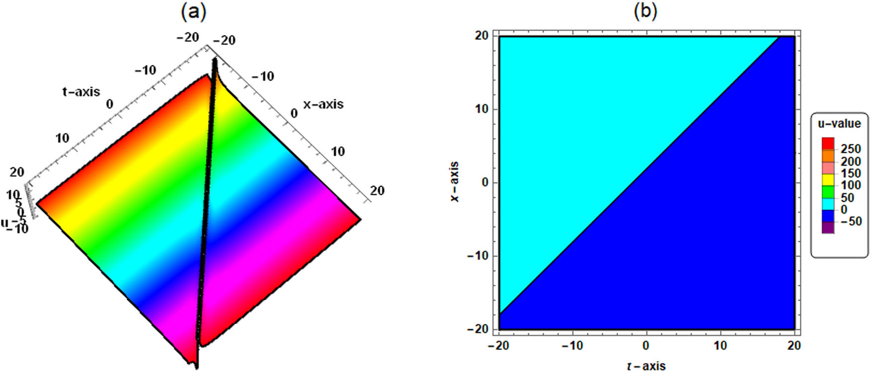
Substituting Eqs (4) and (5) in Eq. (2), the rational solutions are provided by

(6) u = 3 τ 1,1 τ 1,1 ( x − t ) + τ 0,1 + τ 1,0 .

The characteristics of the solution (6) are shown in Figure 1, which clearly shows the structure of an anti-kink solitary wave. This new solution to Eq. (1), found using polynomial methods, has a unique shape with a smooth but sudden change between two different states. Unlike regular kink waves that go up from one balance to another, the anti-kink wave goes down, moves steadily, and keeps its size and shape like solitary waves in nonlinear systems. The solution’s size, speed, and width, given in its formula, show the physical limits of the system. Figure 1 also explains these features with 3D spacetime images and contour analyses, showing the wave’s stable movement and how it switches phases in certain places.

$Figure 1 τ 1,1 = τ 1,0 = 1 {\tau }_{\mathrm{1,1}}={\tau }_{\mathrm{1,0}}=1 , τ 0,1 = − 3 {\tau }_{\mathrm{0,1}}=-3 : (a) three-dimensional plot and (b) contour plot.$

Figure 1

τ 1,1 = τ 1,0 = 1 , τ 0,1 = − 3 : (a) three-dimensional plot and (b) contour plot.

Calculation code for rational solutions:

In [ 1 ] : ϑ ( x , t ) = ∑ i = 1 2 ∑ j = 1 2 τ i j x i t j In [ 2 ] : R = − 9 ϑ ( x , t ) x t ϑ ( x , t ) x x + 2 ϑ ( x , t ) × ( ϑ ( x , t ) x t + ϑ ( x , t ) x x ) + ϑ ( x , t ) x ( 9 ϑ ( x , t ) x x t − 2 ( ϑ ( x , t ) t + ϑ ( x , t ) x ) ) In [ 3 ] : R 1 = FullSimplify [ Coefficient [ R , t 4 x 2 ] ] In [ 4 ] : R 2 = FullSimplify [ Coefficient [ R , x 2 t 2 ] ] In [ 5 ] : R 3 = FullSimplify [ Coefficient [ R , x 2 t ] ] In [ 6 ] : R 3 = FullSimplify [ Coefficient [ R , t 4 ] ] In [ 7 ] : R 4 = FullSimplify [ Coefficient [ R , t 2 ] ] .

3 Double periodic soliton solutions

Building on established solution frameworks [23–25], we construct double periodic soliton solutions for Eq. (1) through the following Ansätz:

(7) ϑ = k 2 e 2 ( δ 4 + β 4 t + α 4 x ) + e δ 1 + β 1 t + α 1 x × [ γ 2 sin ( δ 2 + β 2 t + α 2 x ) + γ 1 cos ( δ 2 + β 2 t + α 2 x ) ] + e δ 3 + β 3 t + α 3 x [ γ 4 sin ( δ 4 + β 4 t + α 4 x ) + γ 3 cos ( δ 4 + β 4 t + α 4 x ) ] + k 1 e 2 ( δ 1 + β 1 t + α 1 x ) ,

where α i , β i , γ i , δ i ( i = 1 , 2, 3, 4) and k j ( j = 1 , 2) are unknown constants. Using Mathematica software, we substitute Eq. (7) in Eq. (3) to derive the following results:

Case (1)

(8) α 4 = k 2 = k 1 = γ 3 = γ 4 = 0 , β 2 = − 2 α 2 9 α 1 2 + 9 α 2 2 + 2 .

Case (2)

(9) α 1 = α 4 , γ 4 = ± γ 3 i , γ 2 = ± γ 1 i , α 3 = ( 2 ∓ i ) α 4 , β 3 = 2 β 1 ∓ i β 4 , β 2 = − α 2 + i α 4 1 + 9 α 4 ( α 4 + i α 2 ) − i β 1 , β 4 = β 1 .

Case (3)

(10) α 1 = α 4 , γ 2 = ± γ 1 i , β 4 = − 2 α 4 9 α 3 2 + 9 α 4 2 + 2 , α 4 = ± α 2 i , α 3 = ( 1 ± 2 i ) α 2 , β 3 = − ( 2 − i ) α 2 ( 18 + 18 i ) α 2 2 − i , β 2 = i α 2 ( 18 + 18 i ) α 2 2 − i , β 1 = α 2 i − ( 18 + 18 i ) α 2 2 .

Case (4)

(11) γ 2 = ∓ γ 1 i , γ 4 = ± γ 3 i , β 4 = 18 α 4 α 1 β 1 + α 1 − α 4 + β 1 18 α 1 α 4 + 1 , α 3 = ( 2 ∓ i ) α 4 , β 2 = − i ( α 1 − α 4 ) 18 α 1 α 4 + 1 − 1 5 − 2 i 5 β 3 , β 1 = α 4 − α 1 18 α 1 α 4 + 1 + 2 5 + i 5 β 3 , α 2 = ± α 1 i .

Case (5)

(12) γ 2 = ± γ 1 i , γ 4 = ± γ 3 i , β 4 = 18 α 4 α 1 β 1 + α 1 − α 4 + β 1 18 α 1 α 4 + 1 , α 4 = 0 , α 2 = ± α 1 i , β 3 = β 2 + i ( α 1 − 2 β 2 ) , α 3 = 2 α 1 , β 1 = ± i β 2 .

By plugging Eq. (7) and Eqs (8)–(12) in Eq. (2), we can obtain a range of periodic soliton solutions. Among them, the breather wave, lump-periodic, and two-wave solutions presented by Tukur et al. [21] are special instances. The physical importance of these solutions is discussed in detail the study by Turkur et al. [21].

Calculation code for double periodic soliton solutions:

In [ 1 ] : ϑ ( x , t ) = k 2 e 2 ( δ 4 + β 4 t + α 4 x ) + e δ 1 + β 1 t + α 1 x [ γ 2 sin ( δ 2 + β 2 t + α 2 x ) + γ 1 cos ( δ 2 + β 2 t + α 2 x ) ] + e δ 3 + β 3 t + α 3 x [ γ 4 sin ( δ 4 + β 4 t + α 4 x ) + γ 3 cos ( δ 4 + β 4 t + α 4 x ) ] + k 1 e 2 ( δ 1 + β 1 t + α 1 x ) In [ 2 ] : M = − 9 ϑ ( x , t ) x t ϑ ( x , t ) x x + 2 ϑ ( x , t ) ( ϑ ( x , t ) x t + ϑ ( x , t ) x x ) + ϑ ( x , t ) x ( 9 ϑ ( x , t ) x x t − 2 ( ϑ ( x , t ) t + ϑ ( x , t ) x ) ) In [ 3 ] : R 1 = FullSimplify [ Coefficient [ M , exp [ 2 ( δ 1 + β 1 t + α 1 x ) + 2 ( δ 4 + β 4 t + α 4 x ) ] ] ] In [ 4 ] : R 2 = FullSimplify [ Coefficient [ M , e 2 δ 3 + 2 β 3 t + 2 α 3 x ] ] In [ 5 ] : R 3 = FullSimplify [ Coefficient [ M , e 3 ( δ 1 + β 1 t + α 1 x ) ] ] In [ 6 ] : R 3 = FullSimplify [ Coefficient [ M , exp [ δ 3 + β 3 t + 2 ( δ 4 + β 4 t + α 4 x ) + α 3 x ] ] ] In [ 7 ] : R 4 = FullSimplify [ Coefficient [ M , e δ 1 + δ 3 + β 1 t + β 3 t + α 1 x + α 3 x ] ] In [ 8 ] : R 5 = FullSimplify [ Coefficient [ M , exp [ δ 3 + β 3 t + 2 ( δ 1 + β 1 t + α 1 x ) + α 3 x ] ] ] In [ 9 ] : R 6 = FullSimplify [ Coefficient [ M , exp [ δ 1 + β 1 t + 2 ( δ 4 + β 4 t + α 4 x ) + α 1 x ] ] ] .

4 Hyperbolic-type and trigonometric-type solutions

Considering the improved ( G ′ ∕ G ) -expansion method, the solution of Eq. (1) can be supposed as a polynomial of ( G ′ ∕ G )

(13) u = ∑ i = − 1 1 a i G ′ G i ,

where G = G ( ξ ) , ξ ( x , t ) = g ( x ) + h ( t ) . g ( x ) , h ( t ) , and a i = a i ( x , t ) ( i = − 1,0,1 ) are unknown functions. Compared to traditional ( G ′ ∕ G ) -expansion method, the function ξ ( x , t ) we use is a nonlinear function that includes nonlinear waves. G satisfies

(14) G ″ + λ G ′ + μ G = 0

with the following solutions

(15) G ′ G = − λ 2 + τ 1 C 1 cosh ( τ 1 ξ ) + C 2 sinh ( τ 1 ξ ) C 1 sinh ( τ 1 ξ ) + C 2 cosh ( τ 1 ξ ) , λ 2 − 4 μ > 0 , τ 1 = λ 2 − 4 μ 2 ,

(16) G ′ G = − λ 2 + τ 2 − C 1 sin ( τ 2 ξ ) + C 2 cos ( τ 2 ξ ) C 1 cos ( τ 2 ξ ) + C 2 sin ( τ 2 ξ ) , λ 2 − 4 μ < 0 , τ 2 = − λ 2 + 4 μ 2 ,

(17) G ′ G = − λ 2 + C 2 C 1 + C 2 ξ , λ 2 − 4 μ = 0 ,

where λ , μ , C 1 , and C 2 are arbitrary constants. Substituting Eqs (13) and (14) in Eq. (1), we have

Case 1:

(18) a − 1 = a 0 = 0 , h ( t ) = t ϱ + ϕ , g ( x ) = x ( ± 1 − 18 μ ϱ 2 − 1 ) 9 μ ϱ , a 1 = ( ± 1 − 18 μ ϱ 2 − 1 ) 9 μ ϱ ,

where ϱ and ϕ are arbitrary constants.

Case 2:

(19) a 1 = a 0 = 0 , h ( t ) = t ϱ + ϕ , g ( x ) = x ( ± 1 − 18 μ ϱ 2 − 1 ) 9 μ ϱ , a − 1 = 1 ± 1 − 18 μ ϱ 2 3 ϱ .

Case 3:

(20) a 0 = 0 , h ( t ) = t ϱ + ϕ , g ( x ) = x ( ± 1 − 72 μ ϱ 2 − 1 ) 36 μ ϱ , a − 1 = 1 ± 1 − 72 μ ϱ 2 12 ϱ , a 1 = − 1 − 72 μ ϱ 2 − 1 12 μ ϱ , λ = 0 .

Substituting Cases 1, 2, 3, and Eqs (15)–(17) in Eq. (13), new hyperbolic-type and trigonometric-type solutions of Eq. (1) are obtained for the first time based on the improved ( G ′ ∕ G ) -expansion method.

Calculation code for hyperbolic-type and trigonometric-type solutions:

In [ 1 ] : u ( x , t ) = a − 1 ( x , t ) G ( ξ ( x , t ) ) G ′ ( ξ ( x , t ) ) + a 1 ( x , t ) G ′ ( ξ ( x , t ) ) G ( ξ ( x , t ) ) + a 0 ( x , t ) In [ 2 ] : M = 1 2 u t u 2 + 3 2 u x t u + u t − 3 2 u t u x + u x In [ 3 ] : R 1 = FullSimplify Coefficient M , G ′ ( ξ ( x , t ) ) 4 G ( ξ ( x , t ) ) 4 In [ 4 ] : R 2 = FullSimplify Coefficient M , G ( ξ ( x , t ) ) 4 G ′ ( ξ ( x , t ) ) 4 In [ 5 ] : R 3 = FullSimplify Coefficient M , G ′ ( ξ ( x , t ) ) 3 G ( ξ ( x , t ) ) 3 In [ 6 ] : R 3 = FullSimplify Coefficient M , G ( ξ ( x , t ) ) 3 G ′ ( ξ ( x , t ) ) 3 In [ 7 ] : R 4 = FullSimplify Coefficient M , G ′ ( ξ ( x , t ) ) 2 G ( ξ ( x , t ) ) 2 In [ 8 ] : R 5 = FullSimplify Coefficient M , G ( ξ ( x , t ) ) 2 G ′ ( ξ ( x , t ) ) 2 In [ 9 ] : R 6 = FullSimplify Coefficient M , G ′ ( ξ ( x , t ) ) G ( ξ ( x , t ) ) In [ 10 ] : R 7 = FullSimplify Coefficient M , G ( ξ ( x , t ) ) G ′ ( ξ ( x , t ) ) In [ 11 ] : R 8 = FullSimplify Coefficient M , G ( ξ ( x , t ) ) G ′ ( ξ ( x , t ) ) , 0 .

5 Interpretation of results

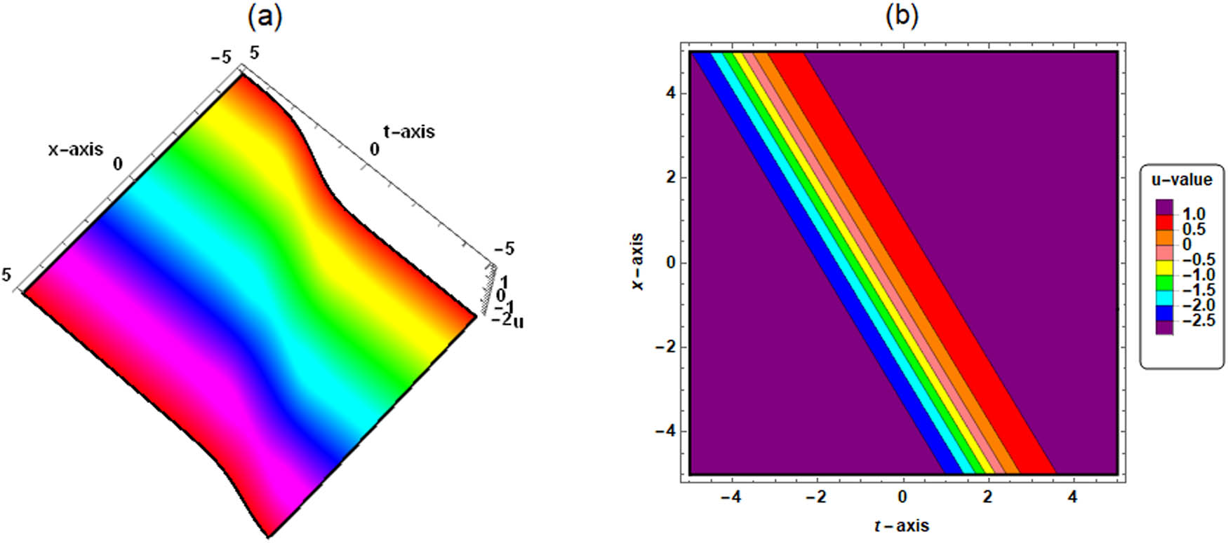
In this section, we intend to demonstrate the dynamic properties of the presented results by some three-dimensional plot and contour plot. Substituting Eqs (15) and (18) in Eq. (13), we derive the following new hyperbolic-type solution:

(21) u = − λ 2 − 4 μ C 2 sinh 1 2 λ 2 − 4 μ t ϱ − x ( 1 − 18 μ ϱ 2 + 1 ) 9 μ ϱ + ϑ + C 1 cosh 1 2 λ 2 − 4 μ t ϱ − x ( 1 − 18 μ ϱ 2 + 1 ) 9 μ ϱ + ϑ × ( 1 − 18 μ ϱ 2 + 1 ) ] ∕ C 1 sinh 1 2 λ 2 − 4 μ t ϱ − x ( 1 − 18 μ ϱ 2 + 1 ) 9 μ ϱ + ϑ + C 2 cosh 1 2 λ 2 − 4 μ t ϱ − x ( 1 − 18 μ ϱ 2 + 1 ) 9 μ ϱ + ϑ − λ ∕ ( 6 μ ϱ ) .

The dynamic properties for solution (21) are shown in Figure 2.

$Figure 2 ϱ = μ = − 1 \varrho =\mu =-1 , C 1 = 0 {C}_{1}=0 , C 2 = 3 {C}_{2}=3 , λ = ϕ = 1 \lambda =\phi =1 : (a) three-dimensional plot and (b) contour plot.$

Figure 2

ϱ = μ = − 1 , C 1 = 0 , C 2 = 3 , λ = ϕ = 1 : (a) three-dimensional plot and (b) contour plot.

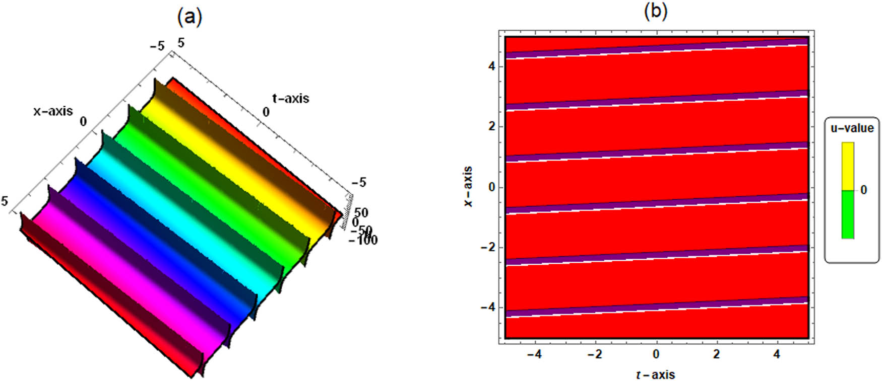
Substituting Eqs (16) and (18) in Eq. (13), we derive the following new trigonometric-type solution:

(22) u = [ ( 1 − 18 μ ϱ 2 + 1 ) [ C 2 ( 4 μ − λ 2 + λ ) × sin 1 2 4 μ − λ 2 t ϱ − x ( 1 − 18 μ ϱ 2 + 1 ) 9 μ ϱ + ϑ + C 1 ( λ − 4 μ − λ 2 ) × cos 1 2 4 μ − λ 2 t ϱ − x ( 1 − 18 μ ϱ 2 + 1 ) 9 μ ϱ + ϑ ∕ 6 μ ϱ C 2 sin 1 2 4 μ − λ 2 t ϱ − x ( 1 − 18 μ ϱ 2 + 1 ) 9 μ ϱ + ϑ + C 1 cos 1 2 4 μ − λ 2 t ϱ − x ( 1 − 18 μ ϱ 2 + 1 ) 9 μ ϱ + ϑ .

The dynamic properties for solution (22) are shown in Figure 3. It is obvious that a periodic solitary wave is shown in Figure 3.

$Figure 3 ϱ = − 0.1 , μ = ϕ = C 1 = λ = 1 , C 2 = 3 \varrho =-0.1,\mu =\phi ={C}_{1}=\lambda =1,{C}_{2}=3 : (a) three-dimensional plot and (b) contour plot.$

Figure 3

ϱ = − 0.1 , μ = ϕ = C 1 = λ = 1 , C 2 = 3 : (a) three-dimensional plot and (b) contour plot.

Drawing code for Figure 3 (The code for other graphics is also similar.):

In[1]: Plot3D[Eq.(22)/.{ ϱ → − 0.1 , C 1 → 1 , C 2 → 3 , λ → 1 , μ → 1 , ϑ → 1 }, { t , − 5,5 } , { x , − 5,5 } , A x e s L a b e l → { ′ ′ t − a x i s ′ ′ , ′ ′ x − a x i s ′ ′ , ′ ′ u ′ ′ } , P l o t L e g e n d s → P l a c e d [ T e x t [ S t y l e [ ′ ′ ( a ) ′ ′ , 20 ] ] , A b o v e ] , P l o t P o i n t s → 100 , V i e w P o i n t → { − 1.765,1.975,6.717 } , B o u n d a r y S t y l e → D i r e c t i v e [ B l a c k , T h i c k ] , C o l o r F u n c t i o n → F u n c t i o n [ { t , x , u , v } , H u e [ x ] ] , L a b e l S t y l e → D i r e c t i v e [ B l a c k , M e d i u m , B o l d ] , M e s h → F a l s e , B o x e d → F a l s e , P l o t R a n g e → A l l ]

In[2]: ContourPlot[Eq.(22)/.{ ϱ → − 0.1 , C 1 → 1 , C 2 → 3 , λ → 1 , μ → 1 , ϑ → 1 }, { t , − 5,5 } , { x , − 5,5 } , F r a m e L a b e l → { t − a x i s , x − a x i s , T e x t [ S t y l e [ ′ ′ ( b ) ′ ′ , 20 ] ] } , P l o t P o i n t s → 180 , P l o t R a n g e → A l l , B o u n d a r y S t y l e → D i r e c t i v e [ B l a c k , T h i c k ] , A x e s L a b e l → { t , x } , L a b e l S t y l e → D i r e c t i v e [ B l a c k , M e d i u m , B o l d ] , C o l o r F u n c t i o n → F u n c t i o n [ { t , x , u , v } , H u e [ x ] ] , P l o t L e g e n d s → B a r L e g e n d [ A u t o m a t i c , L e g e n d M a r k e r S i z e → 120 , L e g e n d F u n c t i o n → ′ ′ F r a m e ′ ′ , L e g e n d M a r g i n s → 5 , L e g e n d L a b e l → ′ ′ u − v a l u e ′ ′ ], C o n t o u r S h a d i n g → { P u r p l e , B l u e , C y a n , G r e e n , Y e l l o w , P i n k , O r a n g e , R e d } ]

6 Conclusion

In this study, the integrable shallow water wave-like equation in coastal engineering has been analyzed using two effective analytical approaches: the polynomial function method and the improved ( G ′ ∕ G ) -expansion method. Several new analytical solutions, including rational, double periodic soliton, hyperbolic-type, and trigonometric-type solutions, have been successfully constructed based on Mathematica software [26–31]. The rational solutions, derived via polynomial functions of x and t , represent anti-kink solitary waves, as illustrated in Figure 1. Meanwhile, the double periodic soliton solutions, obtained through direct functions and symbolic computation, exhibit periodic wave structures, as shown in Figures 2 and 3.

The improved ( G ′ ∕ G ) -expansion method, applied here for the first time to this shallow water wave-like equation, has proven effective in generating diverse solution types. The adopted methods are straightforward and computationally efficient, demonstrating their potential for solving other NLPDEs in engineering and physics. Overall, this work provides a practical framework for deriving analytical solutions to complex wave equations. Future research could extend these methods to higher-dimensional systems to explore more complex physical phenomena.

Funding information: This project was supported by Science and Technology Research Project of Jiangxi Provincial Department of Education (Grant No. GJJ2402805) and Nanchang Institute of Science and Technology Science and Technology Project (Grant No. NGKJ-24-13).
Author contributions: Qing Chen: conceptualization, methodology, software, writing – original draft preparation, and writing – reviewing and editing; Wen-Hui Zhu: methodology, and writing – reviewing and editing. All authors have accepted responsibility for the entire content of this manuscript and approved its submission.
Conflict of interest: The authors state no conflict of interest.
Data availability statement: Data sharing not applicable to this article as no datasets were generated or analyzed during the current study.

References

[1] Hu L, Gao YT, Jia TT, Deng GF, Su JJ. Bilinear forms, N-soliton solutions, breathers and lumps for a (2+1)-dimensional generalized breaking soliton system. Mod Phys Lett B. 2022;36(15):2250033. 10.1142/S0217984922500336Search in Google Scholar

[2] Lan ZZ, Dong S, Gao B, Shen YJ. Bilinear form and soliton solutions for a higher order wave equation. Appl Math Lett. 2022;134:108340. 10.1016/j.aml.2022.108340Search in Google Scholar

[3] Maaa WX. N-soliton solutions and the Hirota conditions in (1+1)-dimensions. Int J Nonlin Sci Num. 2022;23(1):123–33. 10.1515/ijnsns-2020-0214Search in Google Scholar

[4] Feng BF, Ling LM. Darboux transformation and solitonic solution to the coupled complex short pulse equation. Phys D. 2022;437:133332. 10.1016/j.physd.2022.133332Search in Google Scholar

[5] Ma WX. Nonlocal integrable mKdV equations by two nonlocal reductions and their soliton solutions. J Geom Phys. 2022;177:104522. 10.1016/j.geomphys.2022.104522Search in Google Scholar

[6] Guo LJ, Chen L, Mihalache D, He JS. Dynamics of soliton interaction solutions of the Davey-Stewartson I equation. Phys Rev E. 2022;105(1):014218. 10.1103/PhysRevE.105.014218Search in Google Scholar PubMed

[7] He XJ, Lu X. M-lump solution, soliton solution and rational solution to a (3+1)-dimensional nonlinear model. Math Comput Simulat. 2022;197:327–40. 10.1016/j.matcom.2022.02.014Search in Google Scholar

[8] Tian SF, Xu MJ, Zhang TT. A symmetry-preserving difference scheme and analytical solutions of a generalized higher-order beam equation. Proc R Soc A. 2021;477(2255):20210455. 10.1098/rspa.2021.0455Search in Google Scholar

[9] Wazwaz AM. New (3+1)-dimensional integrable fourth-order nonlinear equation: lumps and multiple soliton solutions. Int J Numer Method H. 2022;32(5):1664–73. 10.1108/HFF-05-2021-0318Search in Google Scholar

[10] Liu NN, Wen XY, Wang DS. Dynamics of higher-order rational and semi-rational soliton solutions of the coupled modified KdV lattice equation. Math Method Appl Sci. 2022;45(16):9396–437. 10.1002/mma.8313Search in Google Scholar

[11] Zhang RF, Li MC, Albishari M, Zheng FC, Lan ZZ. Generalized lump solutions, classical lump solutions and rogue waves of the (2+1)-dimensional Caudrey-Dodd-Gibbon-Kotera-Sawada-like equation. Appl Math Comput. 2021;403:126201. 10.1016/j.amc.2021.126201Search in Google Scholar

[12] Wang YN, Niu XX, Liu QP. On the Darboux transformations of the Drinfeld-Sokolov-Satsuma-Hirota coupled KdV system. Rep Math Phys. 2022;90(1):49–62. 10.1016/S0034-4877(22)00050-7Search in Google Scholar

[13] Suuu JJ, Ruan B. N-fold binary Darboux transformation for the nth-order Ablowitz-Kaup-Newell-Segur system under a pseudo-symmetry hypothesis. Appl Math Lett. 2022;125:107719. 10.1016/j.aml.2021.107719Search in Google Scholar

[14] Li Y, Tian SF, Yang JJ. Riemann-Hilbert problem and interactions of solitons in the n-component nonlinear Schrödinger equations. Stud Appl Math. 2022;148(2):577–605. 10.1111/sapm.12450Search in Google Scholar

[15] Biswas A, Sonmezoglu A, Ekici M, Mirzazadeh M, Zhou Q, Alshomrani AS, et al. Optical soliton perturbation with fractional temporal evolution by extended G′∕G-expansion method. Optik. 2018;161:301–20. 10.1016/j.ijleo.2018.02.051Search in Google Scholar

[16] Marwan A, Rahaf A. Convex-periodic, kink-periodic, peakon-soliton and kink bidirectional wave-solutions to new established two-mode generalization of Cahn-Allen equation. Results Phys. 2022;34:105257. 10.1016/j.rinp.2022.105257Search in Google Scholar

[17] Shi, KZ, Ren B, Shen SF, Wang GF, Peng JD, Wang WL, et al. Solitons, rogue waves and interaction behaviors of a third-order nonlinear Schrödinger equation. Results Phys. 2022;37:105533. 10.1016/j.rinp.2022.105533Search in Google Scholar

[18] Wang TY, Zhou Q, Liu WJ. Soliton fusion and fission for the high-order coupled nonlinear Schrödinger system in fiber lasers. Chin Phys B. 2022;31(2):020501. 10.1088/1674-1056/ac2d22Search in Google Scholar

[19] Ma WX. Lump solutions to the Kadomtsev-Petviashvili equation. Phys Lett A. 2015;379:1975–8. 10.1016/j.physleta.2015.06.061Search in Google Scholar

[20] Ma WX, Zhou Y. Lump solutions to nonlinear partial differential equations via Hirota bilinear forms. J Differ Equ. 2018;264:2633–59. 10.1016/j.jde.2017.10.033Search in Google Scholar

[21] Tukur AS, Abdullahi Y, Ali SA, Dumitru B. Lump Collision phenomena to a nonlinear physical model in coastal engineering. Mathematics. 2022;10:2805. 10.3390/math10152805Search in Google Scholar

[22] Zha QL. Rogue waves and rational solutions of a (3+1)-dimensional nonlinear evolution equation. Phys Lett A. 2013;377:3021–6. 10.1016/j.physleta.2013.09.023Search in Google Scholar

[23] Liu JG. Double-periodic soliton solutions for the (3+1)-dimensional Boiti-Leon-Manna-Pempinelli equation in incompressible fluid. Comput Math Appl. 2018;75:3604–13. 10.1016/j.camwa.2018.02.020Search in Google Scholar

[24] Liu JG, Tian Y. New double-periodic soliton solutions for the (2+1)-dimensional breaking soliton equation. Commun Theor Phys. 2018;69:585–97. 10.1088/0253-6102/69/5/585Search in Google Scholar

[25] Liu JG, Zhu WH, Lei ZQ, Ai GP. Double-periodic soliton solutions for the new (2+1)-dimensional KdV equation in fluid flows and plasma physics. Anal Math Phys. 2020;10:41. 10.1007/s13324-020-00387-ySearch in Google Scholar

[26] Zou ZF, Guo R. The Riemann-Hilbert approach for the higher-order Gerdjikov-Ivanov equation, soliton interactions and position shift. Commun Nonlinear Sci Numer Simul. 2023;124:107316. 10.1016/j.cnsns.2023.107316Search in Google Scholar

[27] Zhou Q, Xu MY, Sun YZ, Zhong Y, Mirzazadeh M. Generation and transformation of dark solitons, anti-dark solitons and dark double-hump solitons. Nonlinear Dyn. 2022;110:1747–52. 10.1007/s11071-022-07673-3Search in Google Scholar

[28] Yuan WX, Guo R. Physics-guided multistage neural network: A physically guided network for step initial values and dispersive shock wave phenomena. Phys Rev E. 2025;110:065307. 10.1103/PhysRevE.110.065307Search in Google Scholar PubMed

[29] Chen Y, Yu ZB, Zou L. The lump, lump off and rogue wave solutions of a (2+1)-dimensional breaking soliton equation. Nonlinear Dyn. 2023;111:591–602. 10.1007/s11071-022-07823-7Search in Google Scholar

[30] Huang YH, Guo R. Wave breaking, dispersive shock wave, and phase shift for the defocusing complex modified KdV equation. Chaos. 2024;34:103103. 10.1063/5.0231741Search in Google Scholar PubMed

[31] Liu YH, Guo R, Zhang JW. Inverse scattering transform for the discrete nonlocal PT symmetric nonlinear Schrödinger equation with nonzero boundary conditions. Phys D. 2025;472:134528. 10.1016/j.physd.2024.134466Search in Google Scholar

Received: 2025-05-28

Revised: 2025-08-23

Accepted: 2025-09-04

Published Online: 2025-10-25

This work is licensed under the Creative Commons Attribution 4.0 International License.

Articles in the same Issue

https://doi.org/10.1515/phys-2025-0223

Keywords for this article

mathematica software; (G’/G)-expansion method; symbolic computation; dynamic properties

Creative Commons

BY 4.0