Solitonic wave solutions of a Hamiltonian nonlinear atom chain model through the Hirota bilinear transformation method
-
Baboucarr Ceesay
 and
María G. Medina-Guevara
and
María G. Medina-Guevara

Abstract
This study employs the Hirota bilinear transformation method to investigate solitary and soliton solutions resulting from different symmetry wave functions associated with nonlinear atom chain models. These models are complex dynamic systems that have an impact on a variety of scientific areas. In this work, we derive exact solutions for several symmetry wave functions. Our results reveal a wide range of wave structures, including anti-kink waves (resulting from the interaction of exponential wave functions), M-shaped waves with single and double kinks (generated by combining M-shaped and kink wave functions), and periodic multiple lump waves (produced by the interaction of multi-lump and periodic wave functions). Solitary waves and numerous periodic lump waves have also been reported as a result of various multi-wave function combinations. In the present report, we also derive periodic bright lump waves, periodic cross-kink waves, and dark lump strip waves caused by interactions between exponential, trigonometric, and hyperbolic functions. Additional solutions include solitary waves from mixed wave functions and bright breather waves obtained from homoclinic breather functions. For illustration purposes, we provide three-dimensional visualizations of these solutions as well as accompanying contour plots.
1 Introduction
Nonlinear partial differential equations (NLPDEs) are one of the primary approaches in the modeling and analysis of numerous complex processes [1–3]. These processes include, but are not limited to, plasma physics [4], nonlinear optics [5], chemical kinetics [6], physics of condensed matter [7], and even certain aspects of biology [8]. The reason for this is that NLPDEs are able to catch the dynamics of complex systems with various independent variables. While linear equations possess the property of being relatively simple, NLPDEs embrace the complexities existing within the natural and artificial systems. In this context, one avenue of investigation in NLPDEs is the search for exact solutions which can be used to interpret some physical reality. To that end, many different analytical and numerical approaches have been suggested. Some of the most notable methods involve the modified exp-function method [9], the modified generalized Kudryashov method [10], the extended Jacobi elliptic function rational expansion method [11], Riccati’s equation expansion method [12], the sine-Gordon expansion method [13], the
Among the multiple existing techniques, the Hirota bilinear transformation technique has received special emphasis in view of its application on many complex integrable NLPDEs. This technique is used to convert NLPDEs to bilinear equations, which are easier to deal with. This method allows us to derive soliton solutions, which play an important role in most systems. In the present work, the Hirota bilinear method is used to study solitary and soliton waves in a nonlinear atom chain (NAC) model. It is worth recalling that soliton theory, which is primarily concerned with solitary waves and their propagation, has been quickly established as one of the cornerstones of modern nonlinear physics and mathematics. Solitary waves are a class of waves that can propagate in certain media without changes due to dispersion. These waves propagate and keep their speed for a long time, which is an optimal condition for these waves to be used in describing localized physical processes, such as energy propagation in crystals [25], strain in crystal [26], as well as wave motion in a solid state [27]. Solitary waves have been studied by scientists in many contexts, including aqueous flows, light in fibers, and mechanical waves. For example, some reports investigate solitonic rogue waves induced by the modulation instability in a split-ring-resonator-based left-handed coplanar waveguide [28],
Usually, the behavior of solitary waves is governed by NLPDEs, which are generally complex and often require advance techniques to solve them. What sets these equations apart from their linear counterparts is that they are frequently intractable. Instead, in order to obtain meaningful results, we need sophisticated analytical methods, such as the Hirota bilinear transformation approach or numerical approximations. In many industrial and scientific applications, systems are frequently affected by severe circumstances like high temperatures, high pressures, or fast deformation. The nonlinearities of these equations are essential for capturing those behaviors. Consequently, bettering the design and safety of mechanical systems requires an understanding of nonlinear equations. One area where NLPDEs have proven particularly valuable is in the modeling of NACs. These chains are widely used in the study of materials science and solid mechanics, as they provide insights into the behavior of materials at the atomic level [38–41]. NACs can model a variety of phenomena, including thermal conductivity, wave propagation, defect formation, and material deformation under stress [38,39]. By studying these chains, researchers may obtain a deeper understanding of how materials behave under extreme conditions, leading to the development of high-performance materials for various applications in science, engineering, and technology.
It is also important to point out that wave propagation and solitons in NACs have attracted attention in the last couple of years. In fact, several techniques have been designed to study them rigorously. For instance, Foroutan et al. [42] employed the extended trial equation technique and the improved Bernoulli sub-ordinary differential equation method to solve an NAC problem. They obtained trigonometric, soliton, hyperbolic, and kink solutions. These solutions have applications in generalized momentum for long-range interactions and Hamilton’s equations. In order to analyze NACs, Junaid-U-Rehman et al. [46] made use of the Lie symmetry technique. They generated traveling-wave solutions and utilized the multiplier method to discover the conservation laws. Their results show the dynamics and patterns of the system. Shakeel et al. [47] applied the generalized auxiliary equation method to construct bright, periodic, singular, W-type, and M-type soliton solutions for the NAC model. Among many other reports available in the literature, these solutions form an important aspect in material and structural nanoscience.
On the other hand, the Hirota bilinear transformation technique has made significant contributions to our comprehension of the complex wave solutions produced by various NLPDEs. Notably, a number of researchers have used this technique in recent years to provide exact solutions to a range of NLPDEs. For instance, Ceesay et al. [48] employed the modified regularized long-wave equations to analyze the impact of different M-shaped waves in coastal environments. In order to obtain bilinear equations for NLPDEs with indeterminate coefficients, Yang and Wei [49] also applied Hirota’s bilinear approach. By applying the tanh-coth and Hirota bilinear methods, Wazwaz [50] was able to find many solutions to the Sawada–Kotera–Kadomtsev–Petviashvili model. Furthermore, Rizvi et al. [51] used the Hirota bilinear approach to investigate saturated ferromagnets. Khan and Wazwaz [52] also employed this technique using ansatz functions to derive numerous novel soliton solutions and multi-breather solutions for the Calogero–Bogoyavlenskii–Schiff (CBS) model, whereas Wang et al. [53] adopted a study of plasma and fluid dynamics for the generalized (3 + 1) Kadomtsev–Petviashvili model. Zhao et al. [54] also employed the bilinear approach to produce various lump, mixed lump-stripe solutions using the asymmetric (2 + 1) Nizhnik–Novikov–Veselov model. Using this method, Ren et al. [55] investigated the CBS-type system in the extended (2 + 1) dimensions. In turn, Rizvi and colleagues [56] investigated the coupled Higgs equations using the Hirota bilinear transformation method.
It is worthwhile mentioning that the Hirota bilinear approach extends beyond the traditional study of solitons, and gives margin to study other number of interesting wave forms (including rogue, singular, kink, anti-kink, breather, M-shaped, and lump waves). This fact demonstrates the method’s broad application. These solutions (which are not just theoretical in nature) have real-world applications in fields like biomembrane, fluid dynamics, wave optical pulse, shallow water modeling, etc. Furthermore, given their significant advancements in our knowledge of waves and soliton solutions and their practical applications, these examples show the applicability of the Hirota bilinear technique across fields. In the present study, we departed from the Hirota bilinear transformation method and applied it to an NCA model. After examining earlier research conducted by different investigators who employed the NCA model, they reveal that the Hirota bilinear transformation techniques have not been applied to this system. The purpose of this study is to fill this vacuum in the research literature. In terms of originality, the present work derives novel solutions of an NAC model. Indeed, as some of the reviewers pointed out, there are already some solutions for particular NAC models reported in the literature. However, the investigation of NAC models with an associated Hamiltonian is a problem for which exact solutions have not been derived. Additionally, the Hirota bilinear transformation method has not been employed in those contexts. In that sense, the present work is one of the first in the literature, which tackles the derivation of analytical solutions for NAC models using the methodology proposed by Hirota.
2 Preliminaries
2.1 Physical model
The purpose of this subsection is to provide an overview of the NAC model under investigation. In our physical model, we will assume only one degree of freedom. The Hamiltonian of the system under study is provided by [42]
where
Here the relative displacement between the
Applying Hamilton’s equations to Eqs (1) and (2), we derive the approximate equation of motion
where
If the inter-atom spacing
and
Hence, Eq. (4) can be expressed as the NLPDE given by
with the constants
It is worthwhile to mention that Eq. (7) may find useful applications in the investigation of one-dimensional chains of atoms when they are studied from a microscopic point of view, in which case, the assumption that
2.2 Analytical method
At this stage, we recall the steps of the Hirota bilinear transformation method and apply them to solve Eq. (7) analytically. We start by applying the Cole–Hopf transformation, which is a logarithmic transformation for the dependent variable
where
As a consequence, it follows that
We then consider the function
In this way, we transformed Eq. (7) into the bilinear form
using transformation (12). Here the bilinear operator
Finally, we can write Eq. (13) as
3 Results
Next we will consider various types of forms for the function
3.1 Interaction via double exponents integral equation (IE)
Following the results in the study by Ceesay et al. [57], this wave structure is derived by letting
where
Set 1.
Substituting this constant in Eq. (16) and the outcome in Eq. (12), we obtain
where

The three-dimensional (3D) (a) and contour diagram (b) representing the IE-type wave.
3.2 Interaction of M-shaped rational wave with one kink (M1K)
This wave configuration is provided by using [58]
where
Set 1.
Substituting these values in Eq. (18), and then the resulting equation in Eq. (12), we obtain
where
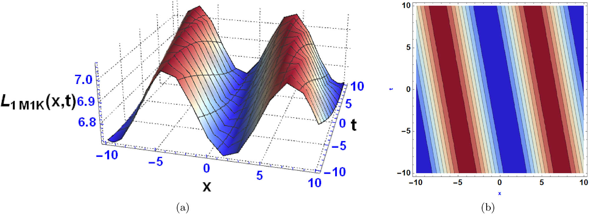
The 3D (a) and contour diagram (b) of M1K wave-type.
3.3 Interaction of M-shaped rational wave with two kinks (M2K)
This wave configuration is provided by [58]
where
Set 1.
After inserting these values in Eq. (20) and the outcome in Eq. (12), we readily obtain
where

The 3D (a) and contour diagram (b) of M2K wave-type.
3.4 Interaction of multi-lump and periodic solutions (MLP)
This wave configuration is provided by [52]
where
Set 1.
Substituting these parameter values in Eq. (22) and then the result in Eq. (12), we obtain
where

The 3D (a) and contour diagram (b) are obtained from the MLP wave-type.
3.5 Multi waves (MU)
This pattern of waves is derived when [59]
where
Set 1.
Substituting them in Eq. (24), and then the result in Eq. (12), yields the solution
where

The 3D (a) and contour diagram (b) of MU wave-type.
Set 2.
Substituting them in Eq. (24) and then the result in Eq. (12), we obtain
where

The 3D (a) and contour diagram (b) of MU wave-type.
3.6 Periodic lump (PL)
This wave structure is given by [59]
where
Set 1.
By replacing these parameter values in Eq. (27), and the outcome in Eq. (12), we obtain
where
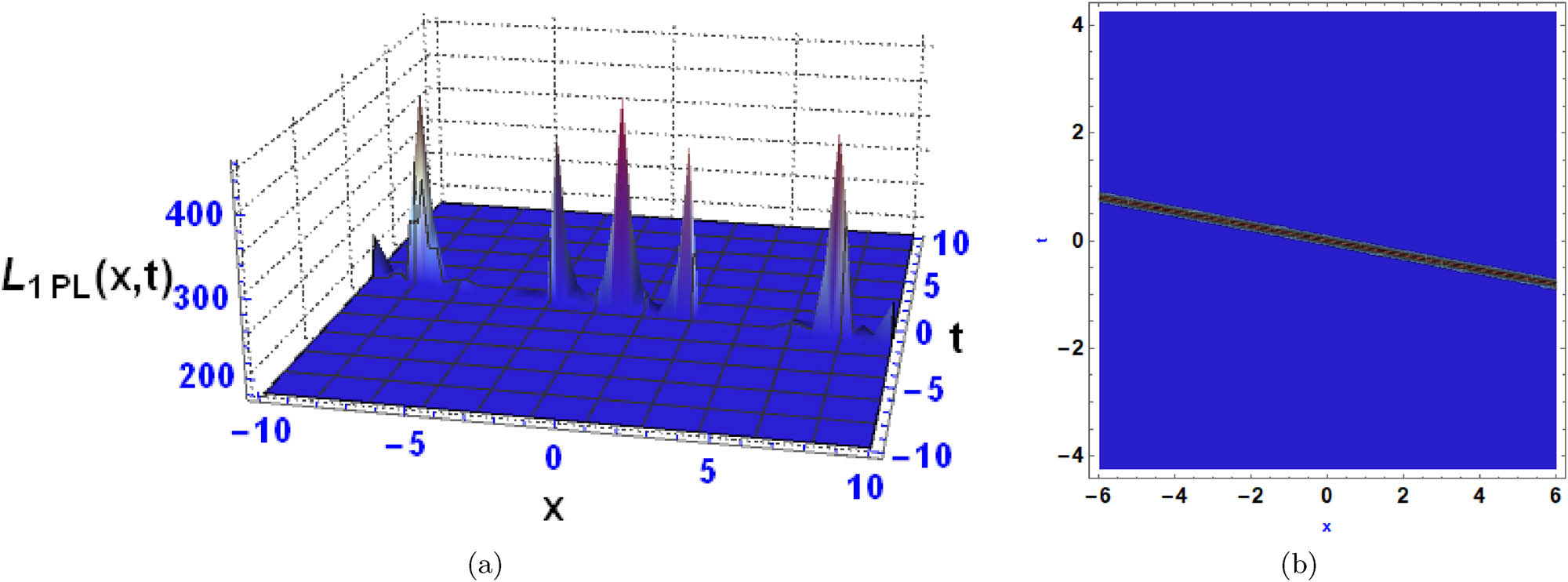
The 3D (a) and contour diagram (b) obtained from PL type wave.
3.7 Periodic cross kink (PCK)
This type of solution is obtained when [59]
where
Set 1.
Inserting them in Eq. (29) and then the outcome in Eq. (12), we have
where
and

The 3D (a) and contour diagram (b) representing the PCK-type wave.
Set 2.
Plugging these parameter values in Eq. (29) and then the result in Eq. (12), we readily reach
The solution

The 3D (a) and contour diagram (b) representing the PCK-type wave.
3.8 Interactions of exponential, trigonometric, and tanh (ETH)
This wave structure is given by [60]
where
Set 1.
By replacing them in Eq. (34) and the outcome in Eq. (12), we obtain
where
and

The 3D (a) and contour diagram (b) representing the ETH-type wave.
3.9 Mixed waves (MI)
This pattern of waves is derived by letting [61]
where
Set 1.
In this case, we derive the solution
where
and
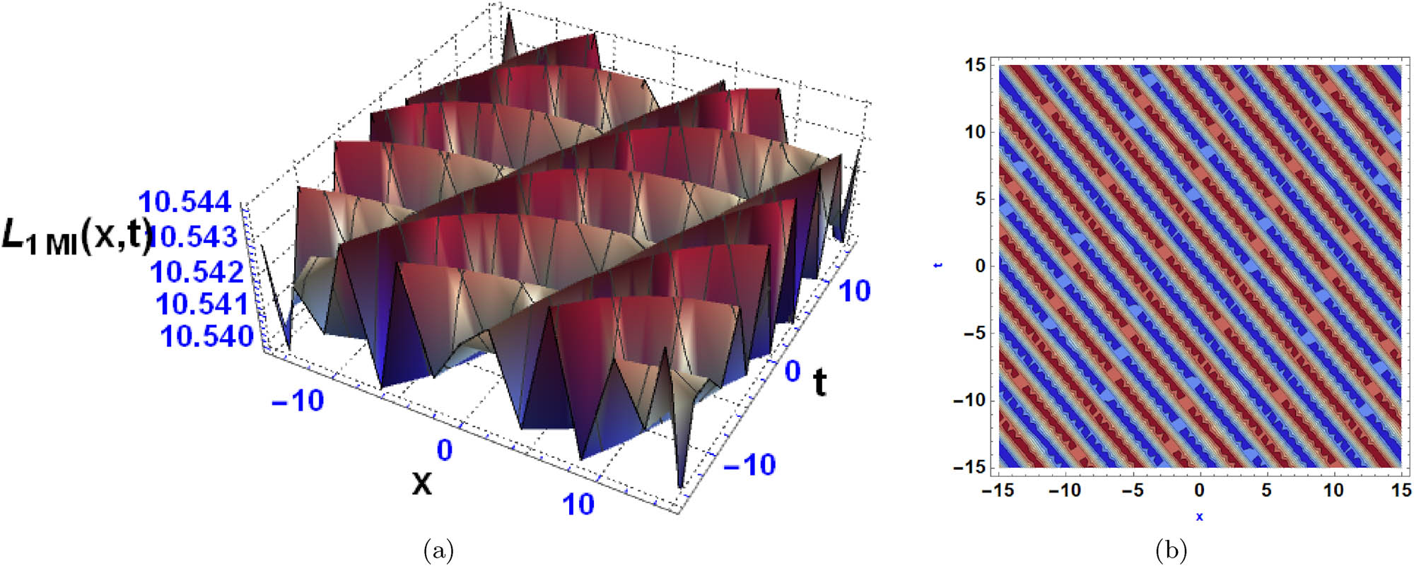
The 3D (a) and contour diagram (b) representing the MI-type wave.
Set 2.
In this case, we obtain the solution
where
and

The 3D (a) and contour diagram (b) representing the MI-type wave.
3.10 Homoclinic breather (HB)
This pattern of waves is reached when [61]
where
Set 1.
Inserting them in Eq. (45) and then the outcome in Eq. (12), we obtain
where
and

The 3D (a) and contour diagram (b) representing the HB-type wave.
Set 2.
In this case, we derive the exact solution
where

The 3D (a) and contour diagram (b) representing the HB-type wave.
4 Discussion
Beforehand, it is important to point out that the functions obtained in Section 3 were substituted into the mathematical model using Mathematica software. The results confirm that, indeed, the functions are solutions of our mathematical model. The 3D graphs and their corresponding contour plots for the solutions derived in the previous section were obtained using Mathematica. The graphs are displayed in Figures 1–14 in order to help in visualizing the characteristic of the solutions. Figure 1(a) shows an anti-kink wave obtained from an interaction between two exponential wave functions. Figure 2(a) shows an M-shaped wave with single kink obtained from an interaction between one M-shaped and one kink wave functions. In Figure 3(a), an M-shaped wave with double kinks is portrayed arising from the wave function of M-shaped and two kinks interactions. Figure 4(a) depicts multiple PL waves obtained from the interaction of multi-lump and periodic wave functions. In turn, Figure 5(a) shows a solitary wave derived from a multi wave function, and Figure 6(a) show multiple PL waves obtained from multi wave functions. Figure 7(a) shows periodic bright lump waves obtained from PL wave structures. Figures 8(a) and 9(a) show PCK waves. In Figure 10(a), we have three dark lump strip waves obtained from the interactions of ETH functions. In Figures 11(a) and 12(a), we obtained solitary waves solutions derived from mixed wave functions. In Figure 13(a), we witnessed three bright breather waves from the HB function, whereas in Figure 14(a) we obtained a single layer of bright breather from the same HB wave function. In each case, Figures 1(b) through 14(b) show the corresponding contour plots. These plots assist in the visualization of the wave profiles by displaying changes in both shape and intensity in different spatial areas at different times. Moreover, concrete physical interpretations of these solutions could be provided by scientists in the context of atomic physics.
These wave phenomena obtained from an atomic chain model each represent distinct physical behaviors. The anti-kink wave transitions between two states in a smooth, sharp manner, but the M-shaped wave with a single kink has a peak structure and a sharp transition point, suggesting localized energy concentration. The M-shaped wave with multiple kinks increases complexity with two abrupt transitions, resulting in steeper atomic movement. Periodic multiple lump waves result from multi-lump and periodic wave interactions, with recurrent localized disruptions indicating oscillating energy. Solitary waves travel without changing form and indicate steady energy transmission across the chain, whereas multiple PL waves cause these localized disruptions to repeat on a regular basis. Periodic bright lump waves identify places with significant energy concentration. PCK waves are the outcome of multidimensional kink interactions that generate crossing wave structures. Dark lump strip waves have a lesser intensity resulting in localized amplitude depressions. Solitary wave solutions formed from mixed wave functions exhibit stable, non-dispersive wave forms. Bright breather waves and their single-layer counterparts show localized, periodic energy variations as they surface in and out over time. These waves together demonstrate complicated energy transfer and atomic displacement dynamics in nonlinear atomic systems.
5 Conclusion
This work investigated a diverse spectrum of solitary and soliton solutions resulting from various symmetry wave functions in a nonlinear atomic chain model. The Hirota bilinear transformation approach was used to unveil a wide range of complicated wave phenomena, including anti-kink waves, M-shaped interacting with kink waves, and PL waves. The combination of exponential, trigonometric, and hyperbolic functions has demonstrated its efficiency in revealing various wave forms such as bright breather waves, periodic bright lump waves, and dark lump strip waves, all of which are required to understand localized energy dynamics in these systems. The graphical illustrations, which included 3D and contour plots, contributed to a better understanding of waveform behavior by showing how solitary and periodic wave structures change spatially and temporally. These findings may shed light on the mechanics of energy transfer and atomic displacement in nonlinear atomic chains, highlighting both stability and the possibility for complex wave interactions. Finally, this study not only adds to the theoretical framework of wave dynamics in nonlinear systems, but it also has potential applications in fields like condensed matter physics and material science, where understanding wave interactions in atomic structures is critical for developing new technologies. The discoveries pave the way for further research into more complicated wave phenomena and their practical consequences in advanced scientific and industrial applications.
As a follow-up to this work, various avenues of research are still open. For instance, the problem of investigating the physical model which considers long-range interactions is an interesting topic of research. In that case, the continuum-limit approximation leads to a fully fractional partial differential equation. In that case, the fractional derivatives appear in the spatial variables. For such system, the derivation of solitary wave solutions and soliton-like solutions is a task that merits attention. In addition, it is worthwhile to point out that the mathematical model studied in the present work is a one-dimensional system in space. This model corresponds to the continuum-limit of a system of particles distributed on a straight line. The case when the atoms are distributed on a plane or inside a three-dimensional volume was not tackled in the present investigation. This is a limitation of our work and, at the same time, a potential direction for future work in the area. Moreover, the elucidation of real-life applications of the results obtained in the present work is also an important problem which needs future attention. Finally, as one of the reviewers pointed out, the exact solutions obtained in this work possess a lot of parameters, and the choice of parameter values to guarantee that a particular solution has a specific wave pattern is certainly a complex task. Such analysis could be the topic of a future report in the context of nonlinear physics.
Acknowledgments
The authors wish to thank the anonymous reviewers and the editor in charge of handling this manuscript for their comments and criticisms. Their suggestions helped in improving substantially the quality of the present report.
-
Funding information: The authors wish to thank the financial support of the University of Guadalajara, Mexico, through the program PROSNI.
-
Author contributions: Conceptualization: N.A. and J.E.M.D.; methodology: B.C., M.Z.B., N.A., J.E.M.D., and S.M.; software: B.C., M.Z.B., N.A., J.E.M.D., and S.M.; validation: B.C., M.Z.B., N.A., J.E.M.D., and S.M.; formal analysis: B.C., M.Z.B., N.A., J.E.M.D., and S.M.; investigation: B.C., M.Z.B., N.A., J.E.M.D., and S.M.; resources, B.C., M.Z.B., N.A., J.E.M.D., and S.M.; data curation, B.C., M.Z.B., N.A., J.E.M.D., and S.M.; writing - original draft preparation, B.C., M.Z.B., N.A., J.E.M.D., and S.M.; writing - review and editing: B.C., M.Z.B., N.A., J.E.M.D. and S.M.; visualization: B.C., M.Z.B., N.A., J.E.M.D., and S.M.; supervision: N.A. and J.E.M.D.; project administration: N.A. and J.E.M.D. All authors have accepted responsibility for the entire content of this manuscript and approved its submission.
-
Conflict of interest: The authors state no conflict of interest.
-
Data availability statement: All data generated or analysed during this study are included in this published article.
References
[1] Briani M, Denaro CA, Piccoli B, Rarità L. Dynamics of particulate emissions in the presence of autonomous vehicles. Open Math. 2025;23(1):20240126. 10.1515/math-2024-0126Search in Google Scholar
[2] Briani M, Manzo R, Piccoli B, Rarità L. Estimation of NOx and O3 reduction by dissipating traffic waves. Netw Heterogeneous Media. 2024;19(2):822–41. 10.3934/nhm.2024037Search in Google Scholar
[3] Rarità L. Optimization approaches to manage congestions for the phenomenon “Luci D’Artista” in Salerno. In Proceedings of 32nd European Modeling and Simulation Symposium, EMSS 2020; 2020. p. 319–24. 10.46354/i3m.2020.emss.046Search in Google Scholar
[4] Alharbi AR, Almatrafi MB, Lotfy K. Constructions of solitary travelling wave solutions for Ito integro-differential equation arising in plasma physics. Results Phys. 2020;19:103533. 10.1016/j.rinp.2020.103533Search in Google Scholar
[5] Agrawal G. P. Nonlinear fiber optics. In Nonlinear science at the dawn of the 21st century. Berlin, Heidelberg: Springer Berlin Heidelberg; 2000. p. 195–211. 10.1007/3-540-46629-0_9Search in Google Scholar
[6] Hafez MG, Kauser MA, Akter MT. Some new exact traveling wave solutions for the Zhiber-Shabat equation. British J Math Comput Sci. 2014;4(18):2582–93. 10.9734/BJMCS/2014/11563Search in Google Scholar
[7] Singh SS. Solutions of Kudryashov-Sinelshchikov equation and generalized Radhakrishnan-Kundu-Lakshmanan equation by the first integral method. Int J Phys Res. 2016;4(2):37–42. 10.14419/ijpr.v4i2.6202Search in Google Scholar
[8] Rawashdeh M. Using the reduced differential transform method to solve nonlinear PDEs arises in biology and physics. World Appl Sci J. 2013;23(8):1037–43. Search in Google Scholar
[9] Shakeel M, Attaullah, Shah NA, Chung JD. Modified exp-function method to find exact solutions of microtubules nonlinear dynamics models. Symmetry. 2023;15(2):360. 10.3390/sym15020360Search in Google Scholar
[10] Liu F, Feng Y. The modified generalized Kudryashov method for nonlinear space-time fractional partial differential equations of Schrödinger type. Results Phys. 2023;53:106914. 10.1016/j.rinp.2023.106914Search in Google Scholar
[11] Chen Y, Wang Q. Extended Jacobi elliptic function rational expansion method and abundant families of Jacobi elliptic function solutions to (1+1)-dimensional dispersive long wave equation. Chaos Solitons Fractals. 2005;24(3):745–57. 10.1016/j.chaos.2004.09.014Search in Google Scholar
[12] Ahmed N, Baber MZ, Iqbal MS, Annum A, Ali SM, Ali M, et al. Analytical study of reaction diffusion Lengyel-Epstein system by generalized Riccati equation mapping method. Sci Rep. 2023;13(1):20033. 10.1038/s41598-023-47207-4Search in Google Scholar PubMed PubMed Central
[13] Kundu PR, Fahim MRA, Islam ME, Akbar MA. The sine-Gordon expansion method for higher-dimensional NLEEs and parametric analysis. Heliyon. 2021;7(3):e06459. 10.1016/j.heliyon.2021.e06459Search in Google Scholar PubMed PubMed Central
[14] Wang M, Li X, Zhang J. The (G′G)-expansion method and travelling wave solutions of nonlinear evolution equations in mathematical physics. Phys Lett A. 2008;372(4):417–23. 10.1016/j.physleta.2007.07.051Search in Google Scholar
[15] Ozisik M, Secer A, Bayram M. On solitary wave solutions for the extended nonlinear Schrödinger equation via the modified F-expansion method. Opt Quantum Electron. 2023;55(3):215. 10.1007/s11082-022-04476-zSearch in Google Scholar
[16] Alsharidi A. K., Bekir A. Discovery of new exact wave solutions to the M-fractional complex three coupled Maccari’s system by Sardar sub-equation scheme. Symmetry. 2023;15(8):1567. 10.3390/sym15081567Search in Google Scholar
[17] Ali A, Ahmad J, Javed S. Dynamic investigation to the generalized Yu-Toda-Sasa-Fukuyama equation using Darboux transformation. Opt Quantum Electron. 2024;56(2):166. 10.1007/s11082-023-05562-6Search in Google Scholar
[18] Abd-Alhalem SM, Marie HS, El-Shafai W, Altameem T, Rathore RS, Hassan TM. Cervical cancer classification based on a bilinear convolutional neural network approach and random projection. Eng Appl Artif Intel. 2024;127:107261. 10.1016/j.engappai.2023.107261Search in Google Scholar
[19] Ali N, Zada L, Nawaz R, Jamshed W, Ibrahim RW, Guedri K, Khalifa HAEW. Analysis and simulation of arbitrary order shallow water and Drinfeld-Sokolov-Wilson equations: Natural transform decomposition method. Int J Modern Phys B, 2024;38(6):2450088. 10.1142/S0217979224500887Search in Google Scholar
[20] Qing W, Pan B. Modified fractional homotopy method for solving nonlinear optimal control problems. Nonl Dyn. 2024;112(5):3453–79. 10.1007/s11071-023-09191-2Search in Google Scholar
[21] Khan M, Hussain M. Application of Laplace decomposition method on semi-infinite domain. Numer Alg. 2011;56:211–8. 10.1007/s11075-010-9382-0Search in Google Scholar
[22] Abdelrazec A, Pelinovsky D. Convergence of the Adomian decomposition method for initial-value problems. Numer Meth Partial Differ Equ. 2011;27(4):749–66. 10.1002/num.20549Search in Google Scholar
[23] Luke JC. A perturbation method for nonlinear dispersive wave problems. Proc R Soc London Ser A Math Phys Sci. 1966;292(1430):403–12. 10.1098/rspa.1966.0142Search in Google Scholar
[24] Zhang RF, Li MC. Bilinear residual network method for solving the exactly explicit solutions of nonlinear evolution equations. Nonl Dyn. 2022;108(1):521–31. 10.1007/s11071-022-07207-xSearch in Google Scholar
[25] Kyame JJ. Wave propagation in piezoelectric crystals. J Acoust Soc Am. 1949;21(3):159–67. 10.1121/1.1906490Search in Google Scholar
[26] Koleshko VM, Meshkov YV, Barkalin VV. Strain effect in single-crystal silicon-based multilayer surface acoustic wave structures. Thin Solid Films. 1990;190(2):359–72. 10.1016/0040-6090(89)90926-7Search in Google Scholar
[27] Priyadarshan P, Rikendra RK. Analysis of wave motion at the solid-solid interface. In: International Conference On Artificial Intelligence Of Things For Smart Societies. Cham: Springer Nature Switzerland; 2024. p. 149–58. 10.1007/978-3-031-63103-0_16Search in Google Scholar
[28] Abbagari S, Houwe A, Akinyemi L, Bouetou TB. Solitonic rogue waves induced by the modulation instability in a split-ring-resonator-based left-handed coplanar waveguide. Chin J Phys 2024;92:1614–27. 10.1016/j.cjph.2023.12.024Search in Google Scholar
[29] Akinyemi L, Manukure S, Houwe A, Abbagari S. A study of (2+1)-dimensional variable coefficients equation: Its oceanic solitons and localized wave solutions. Phys Fluids. 2024;36(1):013120. 10.1063/5.0180078Search in Google Scholar
[30] Akinyemi L, Houwe A, Abbagari S, Wazwaz AM, Alshehri HM, Osman MS. Effects of the higher-order dispersion on solitary waves and modulation instability in a monomode fiber. Optik. 2023;288:171202. 10.1016/j.ijleo.2023.171202Search in Google Scholar
[31] Mukam SPT, Souleymanou A, Kuetche VK, Bouetou TB. Rogue wave dynamics in barotropic relaxing media. Pramana 2018;91:1–4. 10.1007/s12043-018-1633-ySearch in Google Scholar
[32] Abbagari S, Youssoufa S, Tchokouansi HT, Kuetche VK, Bouetou TB, Kofane TC. N-rotating loop-soliton solution of the coupled integrable dispersionless equation. J Appl Math Phys. 2017;5(6):1370–9. 10.4236/jamp.2017.56113Search in Google Scholar
[33] Souleymanou A, Kuetche VK, Bouetou TB, Kofane TC. Traveling wave-guide channels of a new coupled integrable dispersionless system. Commun Theoretic Phys. 2012;57(1):10. 10.1088/0253-6102/57/1/03Search in Google Scholar
[34] Souleymanou A, Kuetche VK, Bouetou TB, Kofane TC. Scattering behavior of waveguide channels of a new coupled integrable dispersionless system. Chin Phys Lett. 2011;28(12):120501. 10.1088/0256-307X/28/12/120501Search in Google Scholar
[35] Seadawy AR, Ahmed HM, Rabie WB, Biswas A. Chirp-free optical solitons in fiber Bragg gratings with dispersive reflectivity having polynomial law of nonlinearity. Optik. 2021;225:165681. 10.1016/j.ijleo.2020.165681Search in Google Scholar
[36] Jhangeer A, Hussain A, Junaid-U-Rehman M, Baleanu D, Riaz MB. Quasi-periodic, chaotic and travelling wave structures of modified Gardner equation. Chaos Solitons Fractals. 2021;143:110578. 10.1016/j.chaos.2020.110578Search in Google Scholar
[37] Braun OM, Kivshar YS. The Frenkel-Kontorova model: concepts, methods, and applications. Vol. 18. Berlin: Springer; 2004. 10.1007/978-3-662-10331-9Search in Google Scholar
[38] Peyrard M, Remoissenet M. Solitonlike excitations in a one-dimensional atomic chain with a nonlinear deformable substrate potential. Phys Rev B. 1982;26(6):2886. 10.1103/PhysRevB.26.2886Search in Google Scholar
[39] Fang X, Wen J, Yin J, Yu D. Wave propagation in nonlinear metamaterial multi-atomic chains based on homotopy method. AIP Adv. 2016;6(12):121706. 10.1063/1.4971761Search in Google Scholar
[40] Khater AH, Callebaut DK, Seadawy AR. General soliton solutions for nonlinear dispersive waves in convective type instabilities. Phys Scr. 2006;74(3):384. 10.1088/0031-8949/74/3/015Search in Google Scholar
[41] Kumar S, Kumar D, Kumar A. Lie symmetry analysis for obtaining the abundant exact solutions, optimal system and dynamics of solitons for a higher-dimensional Fokas equation. Chaos Solitons Fractals. 2021;142:110507. 10.1016/j.chaos.2020.110507Search in Google Scholar
[42] Foroutan M, Zamanpour I, Manafian J. Applications of IBSOM and ETEM for solving the nonlinear chains of atoms with long-range interactions. Europ Phys J Plus. 2017;132:1–18. 10.1140/epjp/i2017-11681-7Search in Google Scholar
[43] Shakeel M, Liu X, Mostafa AM, AlQahtani NF, Alameri A. Dynamic Solitary Wave Solutions Arising in Nonlinear Chains of Atoms Model. J Nonl Math Phys. 2024;31(1):70. Search in Google Scholar
[44] Junaid-U-Rehman M, Kudra G, Awrejcewicz J. Conservation laws, solitary wave solutions, and lie analysis for the nonlinear chains of atoms. Sci Rep. 2023;13(1):11537. Search in Google Scholar
[45] Junaid-U-Rehman M, Kudra G, Awrejcewicz J. Conservation laws, solitary wave solutions, and lie analysis for the nonlinear chains of atoms. Sci Rep. 2023;13(1):11537. Search in Google Scholar
[46] Junaid-U-Rehman M, Kudra G, Awrejcewicz J. Conservation laws, solitary wave solutions, and lie analysis for the nonlinear chains of atoms. Sci Rep. 2023;13(1):11537. 10.1038/s41598-023-38658-wSearch in Google Scholar PubMed PubMed Central
[47] Shakeel M, Liu X, Mostafa AM, AlQahtani NF, Alameri A. Dynamic solitary wave solutions arising in nonlinear chains of atoms model. J Nonl Math Phys. 2024;31(1):70. 10.1007/s44198-024-00231-ySearch in Google Scholar
[48] Ceesay B, Ahmed N, Maciiias-Diiiaz JE. Construction of M-shaped solitons for a modified regularized long-wave equation via Hirota’s bilinear method. Open Phys 2024;22(1):20240057. 10.1515/phys-2024-0057Search in Google Scholar
[49] Yang XF, Wei Y. Bilinear equation of the nonlinear partial differential equation and its application. J Funct Spaces. 2020;2020(1):4912159. 10.1155/2020/4912159Search in Google Scholar
[50] Wazwaz AM. The Hirota’s direct method and the tanh-coth method for multiple-soliton solutions of the Sawada-Kotera-Ito seventh-order equation. Appl Math Comput. 2008;199(1):133–8. 10.1016/j.amc.2007.09.034Search in Google Scholar
[51] Rizvi ST, Seadawy AR, Nimra Ahmad A. Study of lump, rogue, multi, M shaped, periodic cross kink, breather lump, kink-cross rational waves and other interactions to the Kraenkel-Manna-Merle system in a saturated ferromagnetic material. Opt Quantum Electron. 2023;55(9):813. 10.1007/s11082-023-04972-wSearch in Google Scholar
[52] Khan MH, Wazwaz AM. Lump, multi-lump, cross kinky-lump and manifold periodic-soliton solutions for the (2+1)-D Calogero–Bogoyavlenskii–Schiff equation. Heliyon 2020;6(4):e03701. 10.1016/j.heliyon.2020.e03701Search in Google Scholar PubMed PubMed Central
[53] Wang M, Tian B, Qu QX, Zhao XH, Zhang Z, Tian HY. Lump, lumpoff, rogue wave, breather wave and periodic lump solutions for a (3+1)-dimensional generalized Kadomtsev-Petviashvili equation in fluid mechanics and plasma physics. Int J Comput Math. 2020;97(12):2474–86. 10.1080/00207160.2019.1704741Search in Google Scholar
[54] Zhao Z, Chen Y, Han B. Lump soliton, mixed lump stripe and periodic lump solutions of a (2+1)-dimensional asymmetrical Nizhnik-Novikov-Veselov equation. Modern Phys Lett B. 2017;31(14):1750157. 10.1142/S0217984917501573Search in Google Scholar
[55] Ren B, Lin J, Lou ZM. A new nonlinear equation with Lump-Soliton, Lump-Periodic, and Lump-Periodic-Soliton solutions. Complexity. 2019;2019(1):4072754. 10.1155/2019/4072754Search in Google Scholar
[56] Rizvi STR, Seadawy AR, Ashraf MA, Bashir A, Younis M, Baleanu D. Multi-wave, homoclinic breather, M-shaped rational and other solitary wave solutions for coupled-Higgs equation. Europ Phys J Special Topics. 2021;230(18):3519–32. 10.1140/epjs/s11734-021-00270-2Search in Google Scholar
[57] Ceesay B, Baber MZ, Ahmed N, Akgül A, Cordero A, Torregrosa JR. Modelling symmetric ion-acoustic wave structures for the BBMPB equation in fluid ions using Hirota’s bilinear technique. Symmetry. 2023;15(9):1682. 10.3390/sym15091682Search in Google Scholar
[58] Tedjani AH, Seadawy AR, Rizvi ST, Solouma E. Dynamical structure and soliton solutions galore: investigating the range of forms in the perturbed nonlinear Schrödinger dynamical equation. Opt Quant Electron. 2024;56(5):764. 10.1007/s11082-024-06498-1Search in Google Scholar
[59] Ozsahin DU, Ceesay B, Baber MZ, Ahmed N, Raza A, Rafiq M, et al. Multiwaves, breathers, lump and other solutions for the Heimburg model in biomembranes and nerves. Sci Rep. 2024;14(1):10180. 10.1038/s41598-024-60689-0Search in Google Scholar PubMed PubMed Central
[60] Isah MA, Yokus A, Kaya D. Exploring the influence of layer and neuron configurations on Boussinesq equation solutions via a bilinear neural network framework. Nonl Dyn. 2024;112:1–17. 10.1007/s11071-024-09708-3Search in Google Scholar
[61] Ceesay B, Ahmed N, Baber MZ, Akgül A. Breather, lump, M-shape and other interaction for the Poisson-Nernst-Planck equation in biological membranes. Opt Quantum Electron. 2024;56(5):853. 10.1007/s11082-024-06376-wSearch in Google Scholar
© 2025 the author(s), published by De Gruyter
This work is licensed under the Creative Commons Attribution 4.0 International License.
Articles in the same Issue
- Research Articles
- Single-step fabrication of Ag2S/poly-2-mercaptoaniline nanoribbon photocathodes for green hydrogen generation from artificial and natural red-sea water
- Abundant new interaction solutions and nonlinear dynamics for the (3+1)-dimensional Hirota–Satsuma–Ito-like equation
- A novel gold and SiO2 material based planar 5-element high HPBW end-fire antenna array for 300 GHz applications
- Explicit exact solutions and bifurcation analysis for the mZK equation with truncated M-fractional derivatives utilizing two reliable methods
- Optical and laser damage resistance: Role of periodic cylindrical surfaces
- Numerical study of flow and heat transfer in the air-side metal foam partially filled channels of panel-type radiator under forced convection
- Water-based hybrid nanofluid flow containing CNT nanoparticles over an extending surface with velocity slips, thermal convective, and zero-mass flux conditions
- Dynamical wave structures for some diffusion--reaction equations with quadratic and quartic nonlinearities
- Solving an isotropic grey matter tumour model via a heat transfer equation
- Study on the penetration protection of a fiber-reinforced composite structure with CNTs/GFP clip STF/3DKevlar
- Influence of Hall current and acoustic pressure on nanostructured DPL thermoelastic plates under ramp heating in a double-temperature model
- Applications of the Belousov–Zhabotinsky reaction–diffusion system: Analytical and numerical approaches
- AC electroosmotic flow of Maxwell fluid in a pH-regulated parallel-plate silica nanochannel
- Interpreting optical effects with relativistic transformations adopting one-way synchronization to conserve simultaneity and space–time continuity
- Modeling and analysis of quantum communication channel in airborne platforms with boundary layer effects
- Theoretical and numerical investigation of a memristor system with a piecewise memductance under fractal–fractional derivatives
- Tuning the structure and electro-optical properties of α-Cr2O3 films by heat treatment/La doping for optoelectronic applications
- High-speed multi-spectral explosion temperature measurement using golden-section accelerated Pearson correlation algorithm
- Dynamic behavior and modulation instability of the generalized coupled fractional nonlinear Helmholtz equation with cubic–quintic term
- Study on the duration of laser-induced air plasma flash near thin film surface
- Exploring the dynamics of fractional-order nonlinear dispersive wave system through homotopy technique
- The mechanism of carbon monoxide fluorescence inside a femtosecond laser-induced plasma
- Numerical solution of a nonconstant coefficient advection diffusion equation in an irregular domain and analyses of numerical dispersion and dissipation
- Numerical examination of the chemically reactive MHD flow of hybrid nanofluids over a two-dimensional stretching surface with the Cattaneo–Christov model and slip conditions
- Impacts of sinusoidal heat flux and embraced heated rectangular cavity on natural convection within a square enclosure partially filled with porous medium and Casson-hybrid nanofluid
- Stability analysis of unsteady ternary nanofluid flow past a stretching/shrinking wedge
- Solitonic wave solutions of a Hamiltonian nonlinear atom chain model through the Hirota bilinear transformation method
- Bilinear form and soltion solutions for (3+1)-dimensional negative-order KdV-CBS equation
- Solitary chirp pulses and soliton control for variable coefficients cubic–quintic nonlinear Schrödinger equation in nonuniform management system
- Influence of decaying heat source and temperature-dependent thermal conductivity on photo-hydro-elasto semiconductor media
- Dissipative disorder optimization in the radiative thin film flow of partially ionized non-Newtonian hybrid nanofluid with second-order slip condition
- Bifurcation, chaotic behavior, and traveling wave solutions for the fractional (4+1)-dimensional Davey–Stewartson–Kadomtsev–Petviashvili model
- New investigation on soliton solutions of two nonlinear PDEs in mathematical physics with a dynamical property: Bifurcation analysis
- Mathematical analysis of nanoparticle type and volume fraction on heat transfer efficiency of nanofluids
- Creation of single-wing Lorenz-like attractors via a ten-ninths-degree term
- Optical soliton solutions, bifurcation analysis, chaotic behaviors of nonlinear Schrödinger equation and modulation instability in optical fiber
- Chaotic dynamics and some solutions for the (n + 1)-dimensional modified Zakharov–Kuznetsov equation in plasma physics
- Fractal formation and chaotic soliton phenomena in nonlinear conformable Heisenberg ferromagnetic spin chain equation
- Single-step fabrication of Mn(iv) oxide-Mn(ii) sulfide/poly-2-mercaptoaniline porous network nanocomposite for pseudo-supercapacitors and charge storage
- Novel constructed dynamical analytical solutions and conserved quantities of the new (2+1)-dimensional KdV model describing acoustic wave propagation
- Tavis–Cummings model in the presence of a deformed field and time-dependent coupling
- Spinning dynamics of stress-dependent viscosity of generalized Cross-nonlinear materials affected by gravitationally swirling disk
- Design and prediction of high optical density photovoltaic polymers using machine learning-DFT studies
- Robust control and preservation of quantum steering, nonlocality, and coherence in open atomic systems
- Coating thickness and process efficiency of reverse roll coating using a magnetized hybrid nanomaterial flow
- Dynamic analysis, circuit realization, and its synchronization of a new chaotic hyperjerk system
- Decoherence of steerability and coherence dynamics induced by nonlinear qubit–cavity interactions
- Finite element analysis of turbulent thermal enhancement in grooved channels with flat- and plus-shaped fins
- Modulational instability and associated ion-acoustic modulated envelope solitons in a quantum plasma having ion beams
- Statistical inference of constant-stress partially accelerated life tests under type II generalized hybrid censored data from Burr III distribution
- On solutions of the Dirac equation for 1D hydrogenic atoms or ions
- Entropy optimization for chemically reactive magnetized unsteady thin film hybrid nanofluid flow on inclined surface subject to nonlinear mixed convection and variable temperature
- Stability analysis, circuit simulation, and color image encryption of a novel four-dimensional hyperchaotic model with hidden and self-excited attractors
- A high-accuracy exponential time integration scheme for the Darcy–Forchheimer Williamson fluid flow with temperature-dependent conductivity
- Novel analysis of fractional regularized long-wave equation in plasma dynamics
- Development of a photoelectrode based on a bismuth(iii) oxyiodide/intercalated iodide-poly(1H-pyrrole) rough spherical nanocomposite for green hydrogen generation
- Investigation of solar radiation effects on the energy performance of the (Al2O3–CuO–Cu)/H2O ternary nanofluidic system through a convectively heated cylinder
- Quantum resources for a system of two atoms interacting with a deformed field in the presence of intensity-dependent coupling
- Studying bifurcations and chaotic dynamics in the generalized hyperelastic-rod wave equation through Hamiltonian mechanics
- A new numerical technique for the solution of time-fractional nonlinear Klein–Gordon equation involving Atangana–Baleanu derivative using cubic B-spline functions
- Interaction solutions of high-order breathers and lumps for a (3+1)-dimensional conformable fractional potential-YTSF-like model
- Hydraulic fracturing radioactive source tracing technology based on hydraulic fracturing tracing mechanics model
- Numerical solution and stability analysis of non-Newtonian hybrid nanofluid flow subject to exponential heat source/sink over a Riga sheet
- Numerical investigation of mixed convection and viscous dissipation in couple stress nanofluid flow: A merged Adomian decomposition method and Mohand transform
- Effectual quintic B-spline functions for solving the time fractional coupled Boussinesq–Burgers equation arising in shallow water waves
- Analysis of MHD hybrid nanofluid flow over cone and wedge with exponential and thermal heat source and activation energy
- Solitons and travelling waves structure for M-fractional Kairat-II equation using three explicit methods
- Impact of nanoparticle shapes on the heat transfer properties of Cu and CuO nanofluids flowing over a stretching surface with slip effects: A computational study
- Computational simulation of heat transfer and nanofluid flow for two-sided lid-driven square cavity under the influence of magnetic field
- Irreversibility analysis of a bioconvective two-phase nanofluid in a Maxwell (non-Newtonian) flow induced by a rotating disk with thermal radiation
- Hydrodynamic and sensitivity analysis of a polymeric calendering process for non-Newtonian fluids with temperature-dependent viscosity
- Exploring the peakon solitons molecules and solitary wave structure to the nonlinear damped Kortewege–de Vries equation through efficient technique
- Modeling and heat transfer analysis of magnetized hybrid micropolar blood-based nanofluid flow in Darcy–Forchheimer porous stenosis narrow arteries
- Activation energy and cross-diffusion effects on 3D rotating nanofluid flow in a Darcy–Forchheimer porous medium with radiation and convective heating
- Insights into chemical reactions occurring in generalized nanomaterials due to spinning surface with melting constraints
- Influence of a magnetic field on double-porosity photo-thermoelastic materials under Lord–Shulman theory
- Soliton-like solutions for a nonlinear doubly dispersive equation in an elastic Murnaghan's rod via Hirota's bilinear method
- Analytical and numerical investigation of exact wave patterns and chaotic dynamics in the extended improved Boussinesq equation
- Nonclassical correlation dynamics of Heisenberg XYZ states with (x, y)-spin--orbit interaction, x-magnetic field, and intrinsic decoherence effects
- Exact traveling wave and soliton solutions for chemotaxis model and (3+1)-dimensional Boiti–Leon–Manna–Pempinelli equation
- Unveiling the transformative role of samarium in ZnO: Exploring structural and optical modifications for advanced functional applications
- On the derivation of solitary wave solutions for the time-fractional Rosenau equation through two analytical techniques
- Analyzing the role of length and radius of MWCNTs in a nanofluid flow influenced by variable thermal conductivity and viscosity considering Marangoni convection
- Advanced mathematical analysis of heat and mass transfer in oscillatory micropolar bio-nanofluid flows via peristaltic waves and electroosmotic effects
- Exact bound state solutions of the radial Schrödinger equation for the Coulomb potential by conformable Nikiforov–Uvarov approach
- Some anisotropic and perfect fluid plane symmetric solutions of Einstein's field equations using killing symmetries
- Nonlinear dynamics of the dissipative ion-acoustic solitary waves in anisotropic rotating magnetoplasmas
- Curves in multiplicative equiaffine plane
- Exact solution of the three-dimensional (3D) Z2 lattice gauge theory
- Propagation properties of Airyprime pulses in relaxing nonlinear media
- Symbolic computation: Analytical solutions and dynamics of a shallow water wave equation in coastal engineering
- Wave propagation in nonlocal piezo-photo-hygrothermoelastic semiconductors subjected to heat and moisture flux
- Comparative reaction dynamics in rotating nanofluid systems: Quartic and cubic kinetics under MHD influence
- Laplace transform technique and probabilistic analysis-based hypothesis testing in medical and engineering applications
- Physical properties of ternary chloro-perovskites KTCl3 (T = Ge, Al) for optoelectronic applications
- Gravitational length stretching: Curvature-induced modulation of quantum probability densities
- The search for the cosmological cold dark matter axion – A new refined narrow mass window and detection scheme
- A comparative study of quantum resources in bipartite Lipkin–Meshkov–Glick model under DM interaction and Zeeman splitting
- PbO-doped K2O–BaO–Al2O3–B2O3–TeO2-glasses: Mechanical and shielding efficacy
- Nanospherical arsenic(iii) oxoiodide/iodide-intercalated poly(N-methylpyrrole) composite synthesis for broad-spectrum optical detection
- Sine power Burr X distribution with estimation and applications in physics and other fields
- Numerical modeling of enhanced reactive oxygen plasma in pulsed laser deposition of metal oxide thin films
- Dynamical analyses and dispersive soliton solutions to the nonlinear fractional model in stratified fluids
- Computation of exact analytical soliton solutions and their dynamics in advanced optical system
- An innovative approximation concerning the diffusion and electrical conductivity tensor at critical altitudes within the F-region of ionospheric plasma at low latitudes
- An analytical investigation to the (3+1)-dimensional Yu–Toda–Sassa–Fukuyama equation with dynamical analysis: Bifurcation
- Swirling-annular-flow-induced instability of a micro shell considering Knudsen number and viscosity effects
- Numerical analysis of non-similar convection flows of a two-phase nanofluid past a semi-infinite vertical plate with thermal radiation
- MgO NPs reinforced PCL/PVC nanocomposite films with enhanced UV shielding and thermal stability for packaging applications
- Optimal conditions for indoor air purification using non-thermal Corona discharge electrostatic precipitator
- Investigation of thermal conductivity and Raman spectra for HfAlB, TaAlB, and WAlB based on first-principles calculations
- Tunable double plasmon-induced transparency based on monolayer patterned graphene metamaterial
- DSC: depth data quality optimization framework for RGBD camouflaged object detection
- A new family of Poisson-exponential distributions with applications to cancer data and glass fiber reliability
- Numerical investigation of couple stress under slip conditions via modified Adomian decomposition method
- Monitoring plateau lake area changes in Yunnan province, southwestern China using medium-resolution remote sensing imagery: applicability of water indices and environmental dependencies
- Heterodyne interferometric fiber-optic gyroscope
- Exact solutions of Einstein’s field equations via homothetic symmetries of non-static plane symmetric spacetime
- A widespread study of discrete entropic model and its distribution along with fluctuations of energy
- Empirical model integration for accurate charge carrier mobility simulation in silicon MOSFETs
- The influence of scattering correction effect based on optical path distribution on CO2 retrieval
- Anisotropic dissociation and spectral response of 1-Bromo-4-chlorobenzene under static directional electric fields
- Role of tungsten oxide (WO3) on thermal and optical properties of smart polymer composites
- Analysis of iterative deblurring: no explicit noise
- 10.1515/phys-2025-0251
- Review Article
- Examination of the gamma radiation shielding properties of different clay and sand materials in the Adrar region
- Erratum
- Erratum to “On Soliton structures in optical fiber communications with Kundu–Mukherjee–Naskar model (Open Physics 2021;19:679–682)”
- Special Issue on Fundamental Physics from Atoms to Cosmos - Part II
- Possible explanation for the neutron lifetime puzzle
- Special Issue on Nanomaterial utilization and structural optimization - Part III
- Numerical investigation on fluid-thermal-electric performance of a thermoelectric-integrated helically coiled tube heat exchanger for coal mine air cooling
- Special Issue on Nonlinear Dynamics and Chaos in Physical Systems
- Analysis of the fractional relativistic isothermal gas sphere with application to neutron stars
- Abundant wave symmetries in the (3+1)-dimensional Chafee–Infante equation through the Hirota bilinear transformation technique
- Successive midpoint method for fractional differential equations with nonlocal kernels: Error analysis, stability, and applications
- Novel exact solitons to the fractional modified mixed-Korteweg--de Vries model with a stability analysis