Numerical solution of a nonconstant coefficient advection diffusion equation in an irregular domain and analyses of numerical dispersion and dissipation
-
Appanah Rao Appadu
 and
Hagos Hailu Gidey
and
Hagos Hailu Gidey

Abstract
This work is a major extension of our previous work in which we have solved a 2D nonconstant coefficient advection diffusion equation with nonconstant advection and constant diffusion terms on a square domain using the coefficient of dissipation
1 Introduction
The advection diffusion equation is one of the most important partial differential equations in science and it represents a superposition of two different transport processes: advection and diffusion [1,2]. This model is used to describe several physical phenomena such as transport of pollutants [1], flow in porous media [3], water transport in soils [4], mass transfer [5], and heat transfer in a draining film [6].
Several numerical methods have been developed to solve advection diffusion equation with constant coefficients in one, two, and three dimensions (refer [7–14] and references therein).
A novel finite difference scheme following the work of Dehghan [7] is used along with the Crank–Nicolson and Implicit Chapeau function to solve 3D advection diffusion equation with given initial and boundary conditions [13,15]. The authors compare the performance of the three methods by comparing
Nonstandard finite difference methods (NSFDs) are an established class of methods to solve reaction diffusion, advection diffusion partial differential equations in particular. Verma and Kayenat [16] derived an exact finite difference using a solitary wave solution and also proposed a nonstandard finite difference schemes for the generalised Burgers–Huxley equation subject to certain initial and boundary conditions. Some work on comparison of exact finite difference methods and NSFDs for two classes of nonlinear advection diffusion reaction equations and for the nonlinear generalised advection diffusion reaction equations are detailed in the study by Kayenat and Verma [17,18]. Verma and Kayenat constructed NSFD schemes for generalised Burgers–Fisher equation [19]. Nonconstant coefficient partial differential equations have applications in many fields such as: engineering science, quantum mechanics, financial mathematics, isomonodromic deformations, Seiberg–Witten invariants and quantum field theory, shallow water waves, plasmas, solitons, and optics [20]. Using the diffusion damping and the variable coefficient advection methodology, El-Nabulsi [21] concluded that the problem of non-uniform Uranium burnup in nuclear reactor may be reduced.
Hutomo et al. [22] solved an advection diffusion equation using the Du Fort–Frankel method on square and irregular domains. The irregular domain considered is based on the lake of Hasanuddin University. The lake is located at Tamalanrea Campus in Makassar and is of length
Hutomo et al. [22] solved the 2D advection diffusion equation
where
The vector field of the domain of Hasanuddin University lake is shown in Figure 1. To run the numerical experiment, they used the spatial step sizes,
![Figure 1
The vector field of velocity flow of the domain [22].](/document/doi/10.1515/phys-2025-0137/asset/graphic/j_phys-2025-0137_fig_001.jpg)
The vector field of velocity flow of the domain [22].
This study is organised as follows: in Section 2, we describe the numerical experiment considered. In Sections 3, 4, and 5, we construct the three methods namely Lax–Wendroff, Du Fort–Frankel and NSFD and study the stability using approach of Hindmarsch et al. [23] or obtain condition for which the NSFD method replicates positivity of the continuous model. In Section 6, we study the dissipation and dispersion characteristics of Lax–Wendroff scheme. Numerical results are displayed in Section 7. Section 8 highlights the salient features of the study.
2 Numerical experiment
Based on the problem considered by Hutomo et al. [22], which was described in Section 1, we propose to solve the following problem. We solve
where
for
We note that

Domain considered for our study.

Initial profile.
We consider five scenarios.
Scenario 1:
Scenario 2:
Scenario 3:
Scenario 4:
Scenario 5:
For stability, we use the approach of Hindmarsch et al. [23] to find the range of values of
Phase angle along
When
3 Derivation and stability of Lax–Wendroff method
The Lax–Wendroff method when used to discretise Eq. (1) is given by [24]
where
Eq. (2) can be written as
and the amplification factor is
3.1 Scenario 1
A detailed explanation on the stability of Lax–Wendroff scheme for scenario 1 is provided in [24]. We describe briefly some steps involved for the first scenario.
The amplification factor is obtained and we replace
We obtain 3D plots of
![Figure 4
3D plots of the modulus of the amplification factor of Lax–Wendroff scheme vs
x
∈
x\hspace{0.33em}\in
[0, 1] vs
y
∈
y\hspace{0.33em}\in
[0, 1] for
k
=
0.001
k=0.001
, 0.01, 0.1 for scenario 1 and case 1. (a)
k
=
0.001
k=0.001
, (b)
k
=
0.01
k=0.01
, and (c)
k
=
0.1
k=0.1
.](/document/doi/10.1515/phys-2025-0137/asset/graphic/j_phys-2025-0137_fig_004.jpg)
3D plots of the modulus of the amplification factor of Lax–Wendroff scheme vs
![Figure 5
3D plots of the modulus of the amplification factor of Lax–Wendroff scheme vs
x
∈
x\hspace{0.33em}\in
[0, 1] vs
y
∈
y\hspace{0.33em}\in
[0, 1] for
k
=
1.0
k=1.0
, 1.16, 1.18 for scenario 1 and case 1. (a)
k
=
1.0
k=1.0
, (b)
k
=
1.16
k=1.16
, and (c)
k
=
1.18
k=1.18
.](/document/doi/10.1515/phys-2025-0137/asset/graphic/j_phys-2025-0137_fig_005.jpg)
3D plots of the modulus of the amplification factor of Lax–Wendroff scheme vs
We then consider case 2 which is the situation when
Combining inequalities (5) and (6) gives the range of values of
3.2 Scenario 2
We consider Eq. (4) and substitute
3D plots of
![Figure 6
3D plots of the modulus of the amplification factor of Lax–Wendroff scheme vs
x
∈
x\hspace{0.33em}\in
[0, 1] vs
y
∈
y\hspace{0.33em}\in
[0, 1] when
k
=
0.001
k=0.001
, 0.01 for scenario 2 and case 1. (a)
k
=
0.001
k=0.001
and (b)
k
=
0.01
k=0.01
.](/document/doi/10.1515/phys-2025-0137/asset/graphic/j_phys-2025-0137_fig_006.jpg)
3D plots of the modulus of the amplification factor of Lax–Wendroff scheme vs
![Figure 7
3D plots of the modulus of the amplification factor of Lax–Wendroff scheme vs
x
∈
x\hspace{0.33em}\in
[0, 1] vs
y
∈
y\hspace{0.33em}\in
[0, 1] when
k
=
0.015
k=0.015
, 0.016 for scenario 2 and case 1. (a)
k
=
0.015
k=0.015
and (b)
k
=
0.016
k=0.016
.](/document/doi/10.1515/phys-2025-0137/asset/graphic/j_phys-2025-0137_fig_007.jpg)
3D plots of the modulus of the amplification factor of Lax–Wendroff scheme vs
We next make use of Eq. (4) and study stability of the method for case 2. This gives
Hence, the range of values of
3.3 Scenario 3
We consider Eq. (4) and work with case 1, i.e.
The range of values of
![Figure 8
3D plots of the modulus of the amplification factor of Lax–Wendroff scheme vs
x
∈
x\hspace{0.33em}\in
[0, 1] vs
y
∈
y\hspace{0.33em}\in
[0, 1] for some values of
k
k
for scenario 3 and case 1. (a)
k
=
0.001
k=0.001
, (b)
k
=
0.0015
k=0.0015
, and (c)
k
=
0.0016
k=0.0016
.](/document/doi/10.1515/phys-2025-0137/asset/graphic/j_phys-2025-0137_fig_008.jpg)
3D plots of the modulus of the amplification factor of Lax–Wendroff scheme vs
We now consider Eq. (4) for case 2. We obtain
Hence, the range of values of
3.4 Scenario 4
Starting with Eq. (4), we substitute
3D plots of
![Figure 9
3D plots of the modulus of the amplification factor of Lax–Wendroff scheme vs
x
∈
x\hspace{0.33em}\in
[0, 1] vs
y
∈
y\hspace{0.33em}\in
[0, 1] for some values of
k
k
for scenario 4 and case 1. (a)
k
=
0.001
k=0.001
, (b)
k
=
0.0028
k=0.0028
, (c)
k
=
0.0029
k=0.0029
.](/document/doi/10.1515/phys-2025-0137/asset/graphic/j_phys-2025-0137_fig_009.jpg)
3D plots of the modulus of the amplification factor of Lax–Wendroff scheme vs
We then consider case 2. We obtain
Hence, the range of values of
3.5 Scenario 5
Starting with Eq. (4), we substitute
4 Derivation and stability of Du Fort–Frankel method
The Du Fort–Frankel method is a modification of the centred time centred space scheme [22,25] and when used to discretise Eq. (1) is given by [22]
where
The amplification factor satisfies the following equation:
Since
We next use the approach of Hindmarsh et al. [23] to find the range of values of
4.1 Scenario 1
We make use of Eq. (9) and replace
For case 1, fixing
Solving for
For case 2, we obtain the following equation:
For
Combining the two inequalities (10) and (11) gives the range of values of
4.2 Scenario 2
We use (9) and consider case 1. We also replace
Fixing
Solving for
For case 2, we obtain
Solving for
4.3 Scenario 3
For case 1, replacing
Solving
For case 2, replacing
Solving for
4.4 Scenario 4
We consider Eq. (9) and replace
Solving
For case 2, we obtain
and solving for
4.5 Scenario 5
We consider Eq. (9) and replace
Solving for
For case 2, we obtain
and solving for
5 Derivation and stability of NSFD
To construct an NSFD for Eq. (1), we use the following approximations [24]:
where
A single expression for Eq. (12) is given by
We choose the functional relation
We choose
The coefficients of
![Figure 10
3D plots of the coefficients of
C
i
−
1
,
j
n
{C}_{i-1,j}^{n}
and
C
i
,
j
−
1
n
{C}_{i,j-1}^{n}
vs
x
∈
x\hspace{0.33em}\in
[0, 1] vs
y
∈
y\hspace{0.33em}\in
[0, 1] for scenario 1. (a) Coefficient of
C
i
−
1
,
j
n
{C}_{i-1,j}^{n}
and (b) coefficient of
C
i
,
j
−
1
n
{C}_{i,j-1}^{n}
.](/document/doi/10.1515/phys-2025-0137/asset/graphic/j_phys-2025-0137_fig_010.jpg)
3D plots of the coefficients of
![Figure 11
3D plots of the coefficients of
C
i
−
1
,
j
n
{C}_{i-1,j}^{n}
and
C
i
,
j
−
1
n
{C}_{i,j-1}^{n}
vs
x
∈
x\hspace{0.33em}\in
[0, 1] vs
y
∈
y\hspace{0.33em}\in
[0, 1] for scenario 2. (a) Coefficient of
C
i
−
1
,
j
n
{C}_{i-1,j}^{n}
and (b) coefficient of
C
i
,
j
−
1
n
{C}_{i,j-1}^{n}
.](/document/doi/10.1515/phys-2025-0137/asset/graphic/j_phys-2025-0137_fig_011.jpg)
3D plots of the coefficients of
NSFD preserves positivity of the continuous model for scenarios 2–5 when
![Figure 12
3D plots of the coefficients of
C
i
−
1
,
j
n
{C}_{i-1,j}^{n}
and
C
i
,
j
−
1
n
{C}_{i,j-1}^{n}
vs
x
∈
x\hspace{0.33em}\in
[0, 1] vs
y
∈
y\hspace{0.33em}\in
[0, 1] for scenario 3. (a) Coefficient of
C
i
−
1
,
j
n
{C}_{i-1,j}^{n}
and (b) coefficient of
C
i
,
j
−
1
n
{C}_{i,j-1}^{n}
.](/document/doi/10.1515/phys-2025-0137/asset/graphic/j_phys-2025-0137_fig_012.jpg)
3D plots of the coefficients of
![Figure 13
3D plots of the coefficients of
C
i
−
1
,
j
n
{C}_{i-1,j}^{n}
and
C
i
,
j
−
1
n
{C}_{i,j-1}^{n}
vs
x
∈
x\hspace{0.33em}\in
[0, 1] vs
y
∈
y\hspace{0.33em}\in
[0, 1] for scenario 4. (a) Coefficient of
C
i
−
1
,
j
n
{C}_{i-1,j}^{n}
and (b) coefficient of
C
i
,
j
−
1
n
{C}_{i,j-1}^{n}
.](/document/doi/10.1515/phys-2025-0137/asset/graphic/j_phys-2025-0137_fig_013.jpg)
3D plots of the coefficients of
![Figure 14
3D plots of the coefficients of
C
i
−
1
,
j
n
{C}_{i-1,j}^{n}
and
C
i
,
j
−
1
n
{C}_{i,j-1}^{n}
vs
x
∈
x\hspace{0.33em}\in
[0, 1] vs
y
∈
y\hspace{0.33em}\in
[0, 1] for scenario 5. (a) Coefficient of
C
i
−
1
,
j
n
{C}_{i-1,j}^{n}
and (b) coefficient of
C
i
,
j
−
1
n
{C}_{i,j-1}^{n}
.](/document/doi/10.1515/phys-2025-0137/asset/graphic/j_phys-2025-0137_fig_014.jpg)
3D plots of the coefficients of
Range of values of
| Scenario | Lax–Wendroff | Du Fort–Frankel | NSFD |
|---|---|---|---|
| 1 |
|
|
Not positive definite |
| 2 |
|
|
|
| 3 |
|
|
|
| 4 |
|
|
|
| 5 |
|
|
|
6 Numerical dispersion and dissipation of Lax–Wendroff
In this section, we obtain plots of the following quantities vs
modulus of the amplification factor.
relative phase error (RPE).
6.1 Exact amplification factor
We consider Eq. (1) with
Hence,
We now obtain the exact amplification factor denoted as
The modulus of the exact amplification factor is given by
where
6.2 RPE
The RPE is a measure of the dispersive characteristics of a scheme [28]. The RPE is calculated as [28]
where
where
The argument of
The resulting expressions for
Scenario 1 using
Scenario 2 using
Scenario 3 using
Scenario 4 using
Scenario 5 using
6.3 3D plots of
∣
ξ
exact
∣
,
∣
ξ
∣
, RPE vs
ω
x
vs
ω
y
Figures 15, 16, 17, 18, 19, 20, 21, 22, 23, 24 display the plots of modulus of exact amplification factor, modulus of the amplification factor of Lax–Wendroff scheme, RPE of the Lax–Wendroff scheme vs
![Figure 15
3D plots of exact amplification factor and amplification factor vs
ω
x
∈
[
0
,
π
]
{\omega }_{x}\in \left[0,\pi ]
vs
ω
y
∈
[
0
,
π
]
{\omega }_{y}\in \left[0,\pi ]
for the Lax–Wendroff scheme for scenario 1 using
k
=
0.1
k=0.1
and
k
=
0.01
k=0.01
. (a)
k
=
0.1
k=0.1
and (b)
k
=
0.01
k=0.01
.](/document/doi/10.1515/phys-2025-0137/asset/graphic/j_phys-2025-0137_fig_015.jpg)
3D plots of exact amplification factor and amplification factor vs
![Figure 16
3D plots of RPE vs
ω
x
∈
{\omega }_{x}\hspace{0.33em}\in
[0, 1] vs
ω
y
∈
{\omega }_{y}\hspace{0.33em}\in
[0, 1] for the Lax–Wendroff scheme for scenario 1 using
k
=
0.1
k=0.1
and
k
=
0.01
k=0.01
. (a)
k
=
0.1
k=0.1
and (b)
k
=
0.01
k=0.01
.](/document/doi/10.1515/phys-2025-0137/asset/graphic/j_phys-2025-0137_fig_016.jpg)
3D plots of RPE vs
![Figure 17
3D plots of exact amplification factor and amplification factor vs
ω
x
∈
[
0
,
π
]
{\omega }_{x}\in \left[0,\pi ]
vs
ω
y
∈
[
0
,
π
]
{\omega }_{y}\in \left[0,\pi ]
for the Lax–Wendroff scheme for scenario 2 using
k
=
0.01
k=0.01
and
k
=
0.001
k=0.001
. (a)
k
=
0.01
k=0.01
and (b)
k
=
0.001
k=0.001
.](/document/doi/10.1515/phys-2025-0137/asset/graphic/j_phys-2025-0137_fig_017.jpg)
3D plots of exact amplification factor and amplification factor vs
![Figure 18
3D plots of RPE vs
ω
x
∈
{\omega }_{x}\hspace{0.33em}\in
[0, 1] vs
ω
y
∈
{\omega }_{y}\hspace{0.33em}\in
[0, 1] for the Lax–Wendroff scheme for scenario 2 using
k
=
0.01
k=0.01
and
k
=
0.001
k=0.001
. (a)
k
=
0.01
k=0.01
and (b)
k
=
0.001
k=0.001
.](/document/doi/10.1515/phys-2025-0137/asset/graphic/j_phys-2025-0137_fig_018.jpg)
3D plots of RPE vs
![Figure 19
3D plots of exact amplification factor and amplification factor vs
ω
x
∈
[
0
,
π
]
{\omega }_{x}\in \left[0,\pi ]
vs
ω
y
∈
[
0
,
π
]
{\omega }_{y}\in \left[0,\pi ]
for the Lax–Wendroff scheme for scenario 3 using
k
=
0.001
k=0.001
and
k
=
0.0001
k=0.0001
. (a)
k
=
0.001
k=0.001
and (b)
k
=
0.0001
k=0.0001
.](/document/doi/10.1515/phys-2025-0137/asset/graphic/j_phys-2025-0137_fig_019.jpg)
3D plots of exact amplification factor and amplification factor vs
![Figure 20
3D plots of RPE vs
ω
x
∈
{\omega }_{x}\hspace{0.33em}\in
[0, 1] vs
ω
y
∈
{\omega }_{y}\hspace{0.33em}\in
[0, 1] for the Lax–Wendroff scheme for scenario 3 using
k
=
0.001
k=0.001
and
k
=
0.0001
k=0.0001
. (a)
k
=
0.001
k=0.001
and (b)
k
=
0.0001
k=0.0001
.](/document/doi/10.1515/phys-2025-0137/asset/graphic/j_phys-2025-0137_fig_020.jpg)
3D plots of RPE vs
![Figure 21
3D plots of exact amplification factor and amplification factor vs
ω
x
∈
[
0
,
π
]
{\omega }_{x}\in \left[0,\pi ]
vs
ω
y
∈
[
0
,
π
]
{\omega }_{y}\in \left[0,\pi ]
for the Lax–Wendroff scheme for scenario 4 using
k
=
0.001
k=0.001
and
k
=
0.0001
k=0.0001
. (a)
k
=
0.001
k=0.001
and (b)
k
=
0.0001
k=0.0001
.](/document/doi/10.1515/phys-2025-0137/asset/graphic/j_phys-2025-0137_fig_021.jpg)
3D plots of exact amplification factor and amplification factor vs
![Figure 22
3D plots of RPE vs
ω
x
∈
{\omega }_{x}\hspace{0.33em}\in
[0, 1] vs
ω
y
∈
{\omega }_{y}\hspace{0.33em}\in
[0, 1] for the Lax–Wendroff scheme for scenario 4 using
k
=
0.001
k=0.001
and
k
=
0.0001
k=0.0001
. (a)
k
=
0.001
k=0.001
and (b)
k
=
0.0001
k=0.0001
.](/document/doi/10.1515/phys-2025-0137/asset/graphic/j_phys-2025-0137_fig_022.jpg)
3D plots of RPE vs
![Figure 23
3D plots of exact amplification factor and amplification factor vs
ω
x
∈
[
0
,
π
]
{\omega }_{x}\in \left[0,\pi ]
vs
ω
y
∈
[
0
,
π
]
{\omega }_{y}\in \left[0,\pi ]
for the Lax–Wendroff scheme for scenario 5 using
k
=
0.001
k=0.001
and
k
=
0.0001
k=0.0001
. (a)
k
=
0.001
k=0.001
and (b)
k
=
0.0001
k=0.0001
.](/document/doi/10.1515/phys-2025-0137/asset/graphic/j_phys-2025-0137_fig_023.jpg)
3D plots of exact amplification factor and amplification factor vs
![Figure 24
3D plots of RPE vs
ω
x
∈
{\omega }_{x}\hspace{0.33em}\in
[0, 1] vs
ω
y
∈
{\omega }_{y}\hspace{0.33em}\in
[0, 1] for the Lax–Wendroff scheme for scenario 5 using
k
=
0.001
k=0.001
and
k
=
0.0001
k=0.0001
. (a)
k
=
0.001
k=0.001
and (b)
k
=
0.0001
k=0.0001
.](/document/doi/10.1515/phys-2025-0137/asset/graphic/j_phys-2025-0137_fig_024.jpg)
3D plots of RPE vs
7 Numerical results
All numerical experiments are done in MATLAB platform using Dell core i7 machine.
7.1 Scenario 1
From the analysis of stability for the three methods for scenario 1, we find that the Lax–Wendroff and Du Fort–Frankel schemes are stable when

Contour plots of numerical solution vs

Contour plots of numerical solution vs

Contour plots of numerical solution vs

Contour plots of numerical solution vs
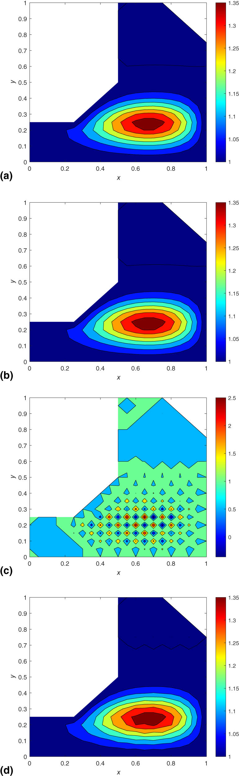
7.2 Results for scenario 2
From Section 4, we find that Lax–Wendroff and Du Fort–Frankel schemes are stable when
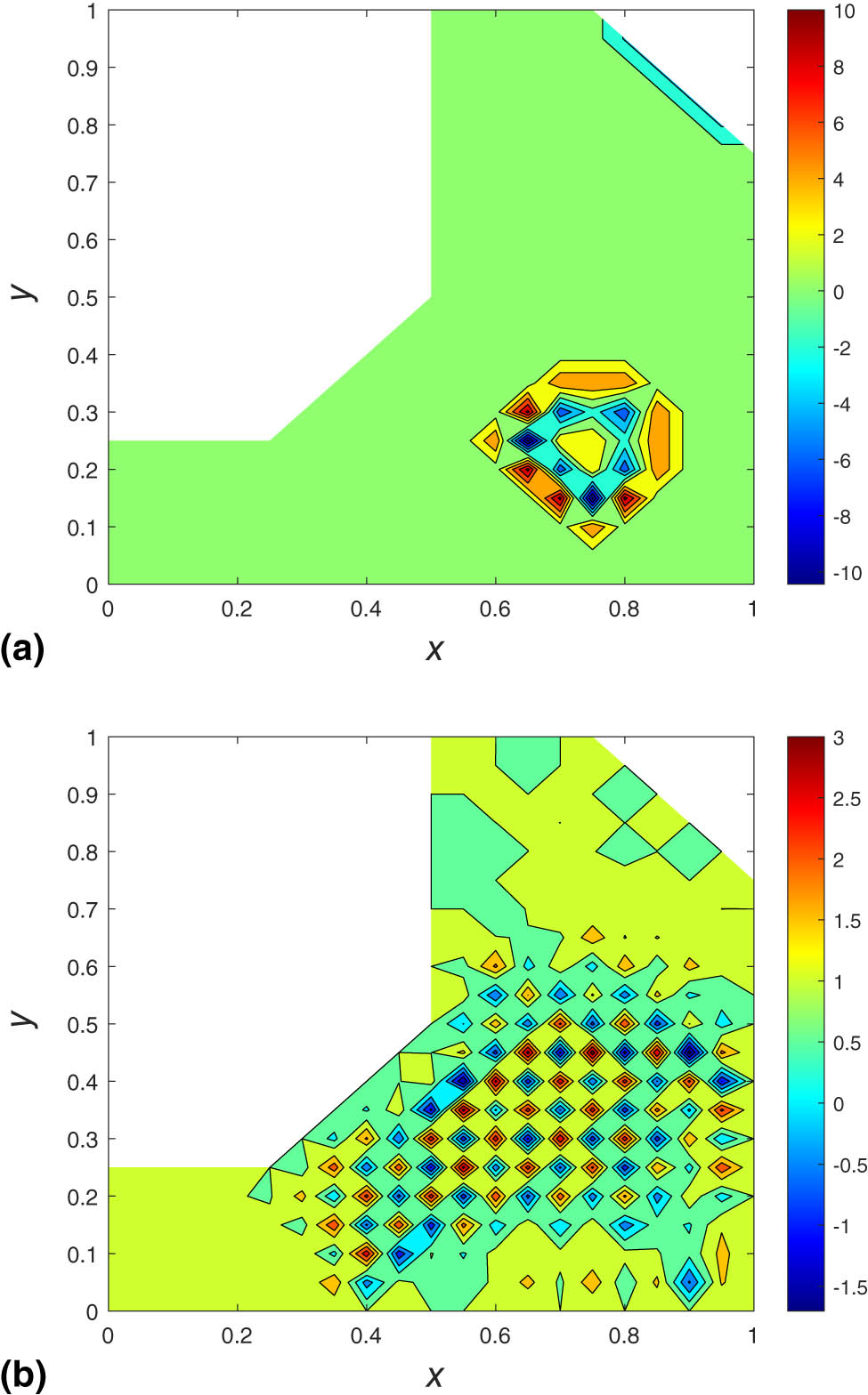
Contour plots of numerical solution vs

Contour plots of numerical solution vs
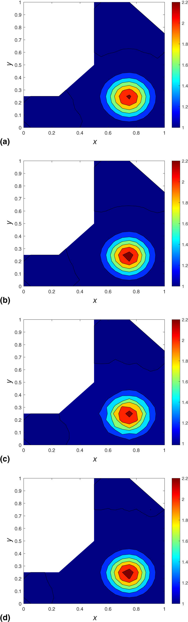
Contour plots of numerical solution vs

Contour plots of numerical solution vs
For scenario 2, NSFD is positive definite and range of numerical solution is 1–3 at time 0.1 and 1–1.25 at time 1. The profiles using Lax–Wendroff and Du Fort–Frankel at
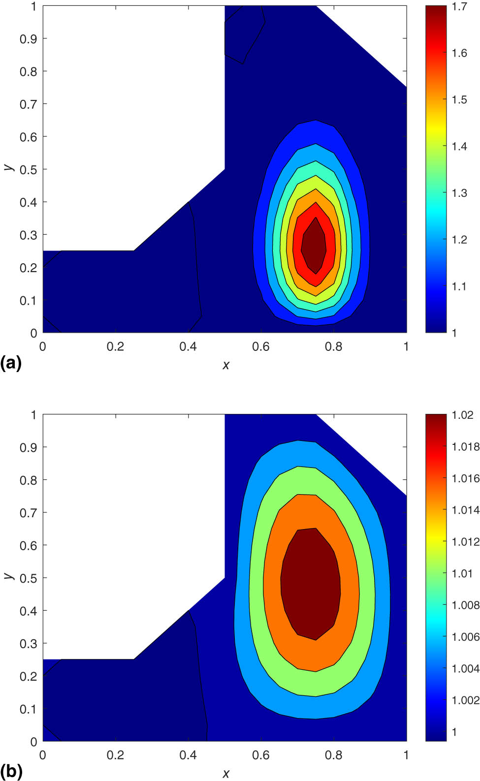
7.3 Results for scenario 3
From the stability analysis, we find that Lax–Wendroff and Du Fort–Frankel are stable when

Contour plots of numerical solution vs

Contour plots of numerical solution vs
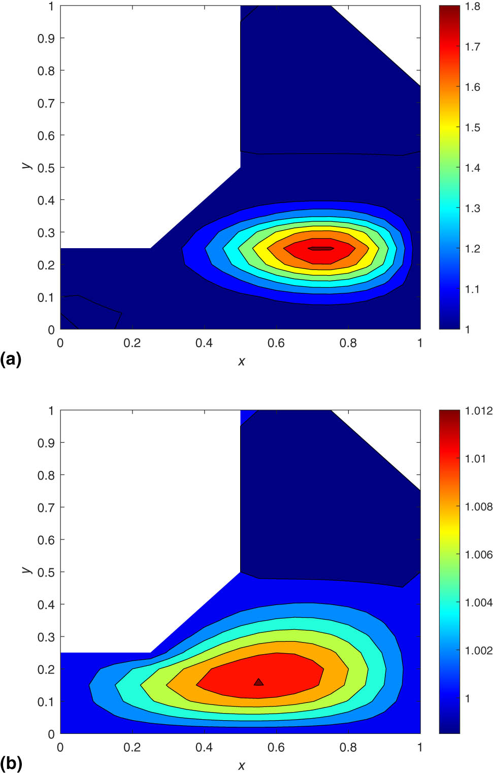
7.4 Results for scenario 4
From the stability analysis, we find that Lax–Wendroff and Du Fort–Frankel are stable when
Contour plots of numerical solution vs

Contour plots of numerical solution vs

Contour plots of numerical solution vs
7.5 Results for scenario 5
From the stability analysis, we find that Lax–Wendroff and Du Fort–Frankel are stable when
Contour plots of numerical solution vs
Contour plots of numerical solution vs

Contour plots of numerical solution vs
8 Conclusion
This work is a major extension of the work by Appadu and Gidey [24] where three numerical schemes, namely, Lax–Wendroff, Du Fort–Frankel and NSFD are used to discretise a 2D nonconstant coefficient advection diffusion equation. A range of values of time-step size of
The Du Fort–Frankel scheme has a much wider range of stability than the Lax–Wendroff scheme. However, it causes considerable dispersive oscillations at values of
Acknowledgments
The authors are grateful to the two anonymous reviewers for the feedback, which enabled them to significantly improve this article in terms of both content and presentation.
-
Funding information: AR Appadu is grateful to Nelson Mandela University (NMU) for allowing him to use his publication funds to pay for open access fees.
-
Author contributions: Both authors have accepted responsibility for the entire content of this manuscript and approved its submission. The plan of the work was provided by AR. Derivation was done by AR. Coding, typing of work was done by HG. Both authors were involved in writing up the paper. Work was supervised by AR. All authors have accepted responsibility for the entire content of this manuscript and approved its submission.
-
Conflict of interest: The authors state no conflict of interest.
-
Data availability statement: All data generated or analysed during this study are included in this published article.
References
[1] Rahaman MM, Takia H, Hasan MK, Hossain MB, Mia S, Hossen K. Application of advection diffusion equation for determination of contaminants in aqueous solution: A mathematical analysis. Appl Math. 2022;10(1):24–31. Search in Google Scholar
[2] Szymkiewicz R. Numerical modeling in open channel hydraulics. vol. 83. Springer Dordrecht; 2010. p. 370.10.1007/978-90-481-3674-2Search in Google Scholar
[3] Kumar N. Unsteady flow against dispersion in finite porous media. J Hydrol. 1983;63(3–4):345–58. 10.1016/0022-1694(83)90050-1Search in Google Scholar
[4] Parlange J. Water transport in soils. Ann Rev Fluid Mech. 1980;12(1):77–102. 10.1146/annurev.fl.12.010180.000453Search in Google Scholar
[5] Guvanasen V, Volker RE. Numerical solutions for solute transport in unconfined aquifers. Int J Numer Meth Fluids. 1983;3(2):103–23. 10.1002/fld.1650030203Search in Google Scholar
[6] Isenberg J, Gutfinger C. Heat transfer to a draining film. Int J Heat Mass Transfer. 1973;16(2):505–12. 10.1016/0017-9310(73)90075-6Search in Google Scholar
[7] Dehghan M. On the numerical solution of the one-dimensional convection-diffusion equation. Math Problems Eng. 2005;2005:61–74. 10.1155/MPE.2005.61Search in Google Scholar
[8] Dehghan M. Time-splitting procedures for the solution of the two-dimensional transport equation. Kybernetes. 2007;36(5/6):791–805. 10.1108/03684920710749857Search in Google Scholar
[9] Shukla A, Singh AK, Singh P. A recent development of numerical methods for solving convection-diffusion problems. Appl Math. 2011;1(1):1–12. 10.5923/j.am.20110101.01Search in Google Scholar
[10] Appadu AR, Djoko JK, Gidey HH. A computational study of three numerical methods for some advection-diffusion problems. Appl Math Comput. 2016;272:629–47. 10.1016/j.amc.2015.03.101Search in Google Scholar
[11] Appadu AR, Gidey HH. Time-splitting procedures for the numerical solution of the 2D advection-diffusion equation. Math Problems Eng. 2013;2013(1):634657. 10.1155/2013/634657.Search in Google Scholar
[12] Dehghan M. Numerical solution of the three-dimensional advection-diffusion equation. Appl Math Comput. 2004;150(1):5–19. 10.1016/S0096-3003(03)00193-0Search in Google Scholar
[13] Appadu AR, Djoko JK, Gidey HH. Performance of some finite difference methods for a 3D advection-diffusion equation. Revista de la Real Academia de Ciencias Exactas, Físicas y Naturales Serie A Matemáticas. 2018;112(4):1179–210. 10.1007/s13398-017-0414-7Search in Google Scholar
[14] Jejeniwa OA, Gidey HH, Appadu AR. Numerical modeling of pollutant transport: Results and optimal parameters. Symmetry. 2022;14(12):2616. 10.3390/sym14122616Search in Google Scholar
[15] Appadu AR, Djoko JK, Gidey HH. Comparative study of some numerical methods to solve a 3D advection-diffusion equation. In: International Conference of Numerical Analysis and Applied Mathematics (ICNAAM 2016). vol. 1863; 2017. p. 030009. 10.1063/1.4992162Search in Google Scholar
[16] Verma AK, Kayenat S. An efficient Mickens’ type NSFD scheme for the generalized Burgers–Huxley equation. J Differ Equ Appl. 2020;26(9–10):1213–46. 10.1080/10236198.2020.1812594Search in Google Scholar
[17] Kayenat S, Verma AK. On the convergence of NSFD schemes for a new class of advection-diffusion-reaction equations. J Differ Equ Appl. 2022;28(7):946–70. 10.1080/10236198.2022.2102425Search in Google Scholar
[18] Kayenat S, Verma AK. Some novel exact and non-standard finite difference schemes for a class of diffusion-advection-reaction equation. J Differ Equ Appl. 2024;30:1–18. 10.1080/10236198.2024.2359106Search in Google Scholar
[19] Kayenat S, Verma AK. NSFD schemes for a class of nonlinear generalised advection-diffusion-reaction equation. Pramana. 2022;96(1):14. 10.1007/s12043-021-02239-1Search in Google Scholar
[20] Strikwerda JC. Finite difference schemes and partial differential equations. Philadelphia: SIAM; 2004. 10.1137/1.9780898717938Search in Google Scholar
[21] El-Nabulsi RA. Neutrons diffusion variable coefficient advection in nuclear reactors. Int J Adv Nucl Reactor Design Tech. 2021;3:102–7. 10.1016/j.jandt.2021.06.005Search in Google Scholar
[22] Hutomo GD, Kusuma J, Ribal A, Mahie AG, Aris N. Numerical solution of 2D advection-diffusion equation with variable coefficient using Du Fort–Frankel method. In: Journal of Physics: Conference Series. vol. 1180. IOP Publishing; 2019. p. 012009. 10.1088/1742-6596/1180/1/012009Search in Google Scholar
[23] Hindmarsh AC, Gresho PM, Griffiths DF. The stability of explicit Euler time-integration for certain finite difference approximations of the multi-dimensional advection-diffusion equation. Int J Numer Methods Fluids. 1984;4(9):853–97. 10.1002/fld.1650040905Search in Google Scholar
[24] Appadu AR, Gidey HH. Stability Analysis and Numerical Results for some schemes discretising 2D nonconstant coefficient advection diffusion equations. Open Phys. 2024;22(1):20230195. 10.1515/phys-2023-0195Search in Google Scholar
[25] Corem N, Ditkowski A. New analysis of the Du Fort–Frankel methods. J Scientif Comput. 2012;53:35–54. 10.1007/s10915-012-9627-2Search in Google Scholar
[26] Tannehill JC, Anderson D, Pletcher R. Computational fluid mechanics and heat transfer. 2nd ed. Washington, DC: Taylor & Francis; 1997. Search in Google Scholar
[27] Appadu AR. Numerical solution of the 1D advection-diffusion equation using standard and nonstandard finite difference schemes. J Appl Math. 2013;2013(1):734374. 10.1155/2013/734374.Search in Google Scholar
[28] Morton KW, Mayers DF. Numerical solution of partial differential equations: an introduction. Cambridge, UK: Cambridge University Press; 2005. 10.1017/CBO9780511812248Search in Google Scholar
© 2025 the author(s), published by De Gruyter
This work is licensed under the Creative Commons Attribution 4.0 International License.
Articles in the same Issue
- Research Articles
- Single-step fabrication of Ag2S/poly-2-mercaptoaniline nanoribbon photocathodes for green hydrogen generation from artificial and natural red-sea water
- Abundant new interaction solutions and nonlinear dynamics for the (3+1)-dimensional Hirota–Satsuma–Ito-like equation
- A novel gold and SiO2 material based planar 5-element high HPBW end-fire antenna array for 300 GHz applications
- Explicit exact solutions and bifurcation analysis for the mZK equation with truncated M-fractional derivatives utilizing two reliable methods
- Optical and laser damage resistance: Role of periodic cylindrical surfaces
- Numerical study of flow and heat transfer in the air-side metal foam partially filled channels of panel-type radiator under forced convection
- Water-based hybrid nanofluid flow containing CNT nanoparticles over an extending surface with velocity slips, thermal convective, and zero-mass flux conditions
- Dynamical wave structures for some diffusion--reaction equations with quadratic and quartic nonlinearities
- Solving an isotropic grey matter tumour model via a heat transfer equation
- Study on the penetration protection of a fiber-reinforced composite structure with CNTs/GFP clip STF/3DKevlar
- Influence of Hall current and acoustic pressure on nanostructured DPL thermoelastic plates under ramp heating in a double-temperature model
- Applications of the Belousov–Zhabotinsky reaction–diffusion system: Analytical and numerical approaches
- AC electroosmotic flow of Maxwell fluid in a pH-regulated parallel-plate silica nanochannel
- Interpreting optical effects with relativistic transformations adopting one-way synchronization to conserve simultaneity and space–time continuity
- Modeling and analysis of quantum communication channel in airborne platforms with boundary layer effects
- Theoretical and numerical investigation of a memristor system with a piecewise memductance under fractal–fractional derivatives
- Tuning the structure and electro-optical properties of α-Cr2O3 films by heat treatment/La doping for optoelectronic applications
- High-speed multi-spectral explosion temperature measurement using golden-section accelerated Pearson correlation algorithm
- Dynamic behavior and modulation instability of the generalized coupled fractional nonlinear Helmholtz equation with cubic–quintic term
- Study on the duration of laser-induced air plasma flash near thin film surface
- Exploring the dynamics of fractional-order nonlinear dispersive wave system through homotopy technique
- The mechanism of carbon monoxide fluorescence inside a femtosecond laser-induced plasma
- Numerical solution of a nonconstant coefficient advection diffusion equation in an irregular domain and analyses of numerical dispersion and dissipation
- Numerical examination of the chemically reactive MHD flow of hybrid nanofluids over a two-dimensional stretching surface with the Cattaneo–Christov model and slip conditions
- Impacts of sinusoidal heat flux and embraced heated rectangular cavity on natural convection within a square enclosure partially filled with porous medium and Casson-hybrid nanofluid
- Stability analysis of unsteady ternary nanofluid flow past a stretching/shrinking wedge
- Solitonic wave solutions of a Hamiltonian nonlinear atom chain model through the Hirota bilinear transformation method
- Bilinear form and soltion solutions for (3+1)-dimensional negative-order KdV-CBS equation
- Solitary chirp pulses and soliton control for variable coefficients cubic–quintic nonlinear Schrödinger equation in nonuniform management system
- Influence of decaying heat source and temperature-dependent thermal conductivity on photo-hydro-elasto semiconductor media
- Dissipative disorder optimization in the radiative thin film flow of partially ionized non-Newtonian hybrid nanofluid with second-order slip condition
- Bifurcation, chaotic behavior, and traveling wave solutions for the fractional (4+1)-dimensional Davey–Stewartson–Kadomtsev–Petviashvili model
- New investigation on soliton solutions of two nonlinear PDEs in mathematical physics with a dynamical property: Bifurcation analysis
- Mathematical analysis of nanoparticle type and volume fraction on heat transfer efficiency of nanofluids
- Creation of single-wing Lorenz-like attractors via a ten-ninths-degree term
- Optical soliton solutions, bifurcation analysis, chaotic behaviors of nonlinear Schrödinger equation and modulation instability in optical fiber
- Chaotic dynamics and some solutions for the (n + 1)-dimensional modified Zakharov–Kuznetsov equation in plasma physics
- Fractal formation and chaotic soliton phenomena in nonlinear conformable Heisenberg ferromagnetic spin chain equation
- Single-step fabrication of Mn(iv) oxide-Mn(ii) sulfide/poly-2-mercaptoaniline porous network nanocomposite for pseudo-supercapacitors and charge storage
- Novel constructed dynamical analytical solutions and conserved quantities of the new (2+1)-dimensional KdV model describing acoustic wave propagation
- Tavis–Cummings model in the presence of a deformed field and time-dependent coupling
- Spinning dynamics of stress-dependent viscosity of generalized Cross-nonlinear materials affected by gravitationally swirling disk
- Design and prediction of high optical density photovoltaic polymers using machine learning-DFT studies
- Robust control and preservation of quantum steering, nonlocality, and coherence in open atomic systems
- Coating thickness and process efficiency of reverse roll coating using a magnetized hybrid nanomaterial flow
- Dynamic analysis, circuit realization, and its synchronization of a new chaotic hyperjerk system
- Decoherence of steerability and coherence dynamics induced by nonlinear qubit–cavity interactions
- Finite element analysis of turbulent thermal enhancement in grooved channels with flat- and plus-shaped fins
- Modulational instability and associated ion-acoustic modulated envelope solitons in a quantum plasma having ion beams
- Statistical inference of constant-stress partially accelerated life tests under type II generalized hybrid censored data from Burr III distribution
- On solutions of the Dirac equation for 1D hydrogenic atoms or ions
- Entropy optimization for chemically reactive magnetized unsteady thin film hybrid nanofluid flow on inclined surface subject to nonlinear mixed convection and variable temperature
- Stability analysis, circuit simulation, and color image encryption of a novel four-dimensional hyperchaotic model with hidden and self-excited attractors
- A high-accuracy exponential time integration scheme for the Darcy–Forchheimer Williamson fluid flow with temperature-dependent conductivity
- Novel analysis of fractional regularized long-wave equation in plasma dynamics
- Development of a photoelectrode based on a bismuth(iii) oxyiodide/intercalated iodide-poly(1H-pyrrole) rough spherical nanocomposite for green hydrogen generation
- Investigation of solar radiation effects on the energy performance of the (Al2O3–CuO–Cu)/H2O ternary nanofluidic system through a convectively heated cylinder
- Quantum resources for a system of two atoms interacting with a deformed field in the presence of intensity-dependent coupling
- Studying bifurcations and chaotic dynamics in the generalized hyperelastic-rod wave equation through Hamiltonian mechanics
- A new numerical technique for the solution of time-fractional nonlinear Klein–Gordon equation involving Atangana–Baleanu derivative using cubic B-spline functions
- Interaction solutions of high-order breathers and lumps for a (3+1)-dimensional conformable fractional potential-YTSF-like model
- Hydraulic fracturing radioactive source tracing technology based on hydraulic fracturing tracing mechanics model
- Numerical solution and stability analysis of non-Newtonian hybrid nanofluid flow subject to exponential heat source/sink over a Riga sheet
- Numerical investigation of mixed convection and viscous dissipation in couple stress nanofluid flow: A merged Adomian decomposition method and Mohand transform
- Effectual quintic B-spline functions for solving the time fractional coupled Boussinesq–Burgers equation arising in shallow water waves
- Analysis of MHD hybrid nanofluid flow over cone and wedge with exponential and thermal heat source and activation energy
- Solitons and travelling waves structure for M-fractional Kairat-II equation using three explicit methods
- Impact of nanoparticle shapes on the heat transfer properties of Cu and CuO nanofluids flowing over a stretching surface with slip effects: A computational study
- Computational simulation of heat transfer and nanofluid flow for two-sided lid-driven square cavity under the influence of magnetic field
- Irreversibility analysis of a bioconvective two-phase nanofluid in a Maxwell (non-Newtonian) flow induced by a rotating disk with thermal radiation
- Hydrodynamic and sensitivity analysis of a polymeric calendering process for non-Newtonian fluids with temperature-dependent viscosity
- Exploring the peakon solitons molecules and solitary wave structure to the nonlinear damped Kortewege–de Vries equation through efficient technique
- Modeling and heat transfer analysis of magnetized hybrid micropolar blood-based nanofluid flow in Darcy–Forchheimer porous stenosis narrow arteries
- Activation energy and cross-diffusion effects on 3D rotating nanofluid flow in a Darcy–Forchheimer porous medium with radiation and convective heating
- Insights into chemical reactions occurring in generalized nanomaterials due to spinning surface with melting constraints
- Influence of a magnetic field on double-porosity photo-thermoelastic materials under Lord–Shulman theory
- Soliton-like solutions for a nonlinear doubly dispersive equation in an elastic Murnaghan's rod via Hirota's bilinear method
- Analytical and numerical investigation of exact wave patterns and chaotic dynamics in the extended improved Boussinesq equation
- Nonclassical correlation dynamics of Heisenberg XYZ states with (x, y)-spin--orbit interaction, x-magnetic field, and intrinsic decoherence effects
- Exact traveling wave and soliton solutions for chemotaxis model and (3+1)-dimensional Boiti–Leon–Manna–Pempinelli equation
- Unveiling the transformative role of samarium in ZnO: Exploring structural and optical modifications for advanced functional applications
- On the derivation of solitary wave solutions for the time-fractional Rosenau equation through two analytical techniques
- Analyzing the role of length and radius of MWCNTs in a nanofluid flow influenced by variable thermal conductivity and viscosity considering Marangoni convection
- Advanced mathematical analysis of heat and mass transfer in oscillatory micropolar bio-nanofluid flows via peristaltic waves and electroosmotic effects
- Exact bound state solutions of the radial Schrödinger equation for the Coulomb potential by conformable Nikiforov–Uvarov approach
- Some anisotropic and perfect fluid plane symmetric solutions of Einstein's field equations using killing symmetries
- Nonlinear dynamics of the dissipative ion-acoustic solitary waves in anisotropic rotating magnetoplasmas
- Curves in multiplicative equiaffine plane
- Exact solution of the three-dimensional (3D) Z2 lattice gauge theory
- Propagation properties of Airyprime pulses in relaxing nonlinear media
- Symbolic computation: Analytical solutions and dynamics of a shallow water wave equation in coastal engineering
- Wave propagation in nonlocal piezo-photo-hygrothermoelastic semiconductors subjected to heat and moisture flux
- Comparative reaction dynamics in rotating nanofluid systems: Quartic and cubic kinetics under MHD influence
- Laplace transform technique and probabilistic analysis-based hypothesis testing in medical and engineering applications
- Physical properties of ternary chloro-perovskites KTCl3 (T = Ge, Al) for optoelectronic applications
- Gravitational length stretching: Curvature-induced modulation of quantum probability densities
- The search for the cosmological cold dark matter axion – A new refined narrow mass window and detection scheme
- A comparative study of quantum resources in bipartite Lipkin–Meshkov–Glick model under DM interaction and Zeeman splitting
- PbO-doped K2O–BaO–Al2O3–B2O3–TeO2-glasses: Mechanical and shielding efficacy
- Nanospherical arsenic(iii) oxoiodide/iodide-intercalated poly(N-methylpyrrole) composite synthesis for broad-spectrum optical detection
- Sine power Burr X distribution with estimation and applications in physics and other fields
- Numerical modeling of enhanced reactive oxygen plasma in pulsed laser deposition of metal oxide thin films
- Dynamical analyses and dispersive soliton solutions to the nonlinear fractional model in stratified fluids
- Computation of exact analytical soliton solutions and their dynamics in advanced optical system
- An innovative approximation concerning the diffusion and electrical conductivity tensor at critical altitudes within the F-region of ionospheric plasma at low latitudes
- An analytical investigation to the (3+1)-dimensional Yu–Toda–Sassa–Fukuyama equation with dynamical analysis: Bifurcation
- Swirling-annular-flow-induced instability of a micro shell considering Knudsen number and viscosity effects
- Numerical analysis of non-similar convection flows of a two-phase nanofluid past a semi-infinite vertical plate with thermal radiation
- MgO NPs reinforced PCL/PVC nanocomposite films with enhanced UV shielding and thermal stability for packaging applications
- Optimal conditions for indoor air purification using non-thermal Corona discharge electrostatic precipitator
- Investigation of thermal conductivity and Raman spectra for HfAlB, TaAlB, and WAlB based on first-principles calculations
- Tunable double plasmon-induced transparency based on monolayer patterned graphene metamaterial
- DSC: depth data quality optimization framework for RGBD camouflaged object detection
- A new family of Poisson-exponential distributions with applications to cancer data and glass fiber reliability
- Numerical investigation of couple stress under slip conditions via modified Adomian decomposition method
- Monitoring plateau lake area changes in Yunnan province, southwestern China using medium-resolution remote sensing imagery: applicability of water indices and environmental dependencies
- Heterodyne interferometric fiber-optic gyroscope
- Exact solutions of Einstein’s field equations via homothetic symmetries of non-static plane symmetric spacetime
- A widespread study of discrete entropic model and its distribution along with fluctuations of energy
- Empirical model integration for accurate charge carrier mobility simulation in silicon MOSFETs
- The influence of scattering correction effect based on optical path distribution on CO2 retrieval
- Anisotropic dissociation and spectral response of 1-Bromo-4-chlorobenzene under static directional electric fields
- Role of tungsten oxide (WO3) on thermal and optical properties of smart polymer composites
- Analysis of iterative deblurring: no explicit noise
- Review Article
- Examination of the gamma radiation shielding properties of different clay and sand materials in the Adrar region
- Erratum
- Erratum to “On Soliton structures in optical fiber communications with Kundu–Mukherjee–Naskar model (Open Physics 2021;19:679–682)”
- Special Issue on Fundamental Physics from Atoms to Cosmos - Part II
- Possible explanation for the neutron lifetime puzzle
- Special Issue on Nanomaterial utilization and structural optimization - Part III
- Numerical investigation on fluid-thermal-electric performance of a thermoelectric-integrated helically coiled tube heat exchanger for coal mine air cooling
- Special Issue on Nonlinear Dynamics and Chaos in Physical Systems
- Analysis of the fractional relativistic isothermal gas sphere with application to neutron stars
- Abundant wave symmetries in the (3+1)-dimensional Chafee–Infante equation through the Hirota bilinear transformation technique
- Successive midpoint method for fractional differential equations with nonlocal kernels: Error analysis, stability, and applications
- Novel exact solitons to the fractional modified mixed-Korteweg--de Vries model with a stability analysis