Explicit exact solutions and bifurcation analysis for the mZK equation with truncated M-fractional derivatives utilizing two reliable methods
-
Pim Malingam


Abstract
The
1 Preliminary background
In recent years, nonlinear partial differential equations (NPDEs) have been employed as models for a wide variety of natural phenomena arising in the physical sciences, biological sciences, and engineering. Because of their importance, they have been investigated in many aspects, for instance, modeling NPDEs from natural rules and facts, constructing and developing efficient analytical and numerical methods for solving NPDEs, and interpreting solutions of NPDEs to explain dynamics of real-world phenomena. Some examples of their applications include the following: the quantum Hall effect [1], wave propagation on the surface of water [2], propagation of solitary waves in optical fibers [3], and nanoscale thermal transportation of ternary magnetized Carreau nanofluid using neural network architecture [4]. Exact traveling waves, including solitary waves and solitons, occur frequently in the real world and play an important role in describing many applications in nonlinear dynamics. A solitary wave is a traveling wave comprising a single peak or trough propagating in isolation whose size, shape, or speed does not change [5]. A solitary water wave is usually found in shallow water.
Over the last few decades, a wide range of NPDE models have been extensively studied in terms of their exact traveling wave solutions using many different approaches including the improved generalized Riccati equation method [6], the new extended direct algebraic method [7], the generalized Kudryashov scheme [8], the modified exponential function method [9], the
The two-dimensional (2D) Zakharov–Kuznetsov (ZK) equation [12] was initially proposed by two Russian mathematicians, namely, Zakharov and Kuznetsov in 1974. It is the canonical 2D extension of the well-known Korteweg-de Vries (K-dV) equation [13]. The ZK equation is a model for weakly nonlinear ion-acoustic waves in intensive geophysical flows and magnetized undamaged plasma in two dimensions. The ZK equation is also used as a model for vulnerable nonlinear ion-acoustic waves arising in a mixture of hot isothermal electrons and cool ions in a uniform magnetic field [14,15]. In addition, this equation has broad applications in mathematical physics and engineering in areas, including ionic temperature, density gradient of ions, existence of dust, compound phenomena in 2D discrete electrical lattices, and inclined propagation. Further details for the ZK equation can be found in previous studies [16–18] and references therein. In recent years, fractional-order ZK models have also been studied with fractional derivatives, including the modified Riemann–Liouville fractional derivative and conformable fractional derivatives [16,19].
The modified Zakharov–Kuznetsov (mZK) equation was first proposed in 1999 [20,21]. The mZK equation is as follows:
where
Recently, there have been many applications of the truncated M-fractional partial derivatives in well-known equations arising in mathematical biology, physics, and engineering research fields. For example, Zhang et al. [22] investigated the dynamical behaviors of nonlinear traveling waves for the generalized reaction Duffing model and density-dependent diffusion–reaction equation in the sense of the M-fractional derivative with respect to temporal and spatial variables. The authors employed the newly extended direct algebraic technique to obtain new exact solutions expressed in terms of rational, hyperbolic, and trigonometric functions. In the study of Siddique et al. [23], the
In this study, the mZK Eq. (1) is modified by changing its partial derivatives to the truncated M-fractional partial derivatives for both time and space dimensions. After applying the truncated M-fractional partial derivatives to (1), we obtain the space–time fractional mZK equation given by
where
In this article, our main aim is to use two reliable methods, namely, the
2 Methodology
In this section, the truncated one-parameter M-fractional derivative is defined and its main characteristics are described. The details of the
2.1 Truncated M-fractional derivative and its characteristics
Here, definitions of the truncated one-parameter MLF and its derivative are provided. Also, the important properties of the derivative are given.
Definition 2.1
The truncated one-parameter MLF is defined as follows [33–36]:
where
Definition 2.2
Let
where
Some useful characteristics of the derivative (4) are as follows [33,36–42]. Let
2.2 Methods
In this subsection, the algorithms of the
where
where the constants
where the polynomial
2.2.1
(
G
′
∕
G
,
1
∕
G
)
-expansion technique
Before giving an algorithm of the
where
Then, using Eq. (9), we can convert Eq. (8) into the system of two nonlinear first-order ODEs
Explicit solutions of Eq. (8) depend on values of
Case 1: When
with the following relationship:
where
Case 2: When
and the associated relation for this case is
where
Case 3: When
with the following associated relation:
where
The main steps of the
Step 1: A solution of Eq. (7) is assumed to be a polynomial of
where
The description of Steps 2–5 of the method is the same as Steps 2–5 of our previous publication [42]. We will omit these steps here to avoid repetition.
2.2.2 Sardar subequation approach
In this subsection, the main steps of the Sardar subequation method [11,49–52] are briefly described as follows.
Step 1: After transforming Eq. (5) into Eq. (7) via the transformation (6), we set up, by the Sardar method, a solution of Eq. (7) as
where
where constants
Case 1: If
where
Case 2: If
where
Case 3: If
where
Case 4: If
where
Step 2: Compute the value of
Step 3: Replacing the value of
Step 4: The exact solutions of Eq. (5) can then be derived by replacing the wave transformation (6), the solutions
These two reliable methods are simple to implement and can provide abundant solutions to the NPDEs, including hyperbolic, trigonometric, and exponential rational functions.
3 Implementation of the schemes
This section investigates the use of the two analytical approaches, namely, the
where the traveling wave transformation
where
Substituting solutions (24) and (25) into the proposed problem (2) and using the properties of the derivative of
Integrating Eq. (26) with regard to
Using the balance principle and the degree formulas expressed in the study of Malingam et al. [42], we obtain the balance number
3.1 Application of the
(
G
′
∕
G
,
1
∕
G
)
-expansion scheme
Following the
where
Case 1 (
Using Maple 17 to solve the aforementioned system, we then obtain the outputs as follows:
Result 1
where
where
Result 2
where
where
Result 3
where
where
Case 2 (
Utilizing Maple 17 to solve the aforementioned system, we have
Result 1
where
where
Result 2
where
where
Case 3 (
Utilizing Maple 17 to solve the aforementioned system, it results in an impractical case, i.e.,
3.2 Application of the Sardar subequation technique
In this section, explicit exact solutions of Eq. (2) are obtained using the Sardar subequation method. Based on the method described in Section 2.2.2, we assume that a solution form of Eq. (27) with
where
Solving system (40) using Maple 17, we obtain the following result:
where
Case 1: when
where
Case 2: When
where
Case 3: When
where
Case 4: When
where
4 Bifurcation analysis and chaotic behavior
This section is devoted to analyzing the bifurcations [24,53,54] of Eq. (27). To achieve this, we employ the Galilean transformation to transform Eq. (27) to an equivalent dynamical system. Later, we will analyze the phase portraits of the corresponding dynamical system whose behaviors can be studied using MATLAB. Now, defining
The phase portrait analysis depends on the dynamical behavior of system (46). Moreover, on the basis of the phase plane, we can plot different trajectories to show the potential state of the aforementioned system. We proceed to derive the auxiliary Hamiltonian function, which is considered as the first integral of system (46) given by
where
whose determinant is
It is known from the theory of planar dynamical systems that we can analyze the equilibrium point
If
If
If
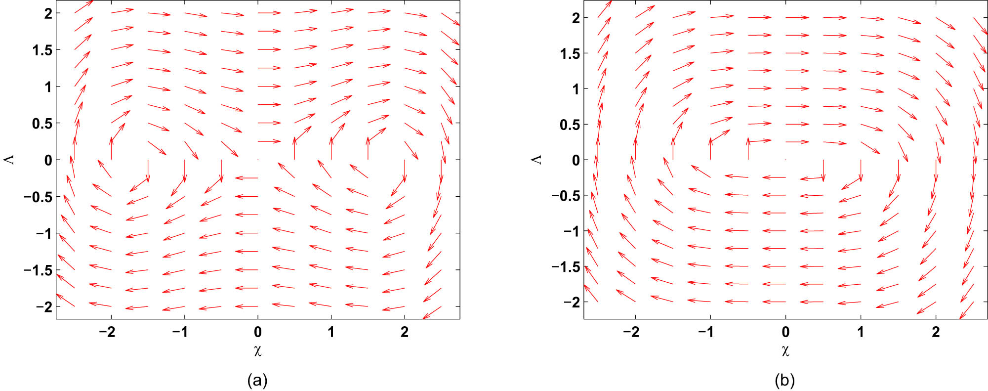
(a) and (b) Bifurcation of phase portrait for system (46) by varying the parameter
Next, we aim to investigate the chaotic behavior of system (46). To achieve that, we have to add a periodic external force to system (46) to become
where
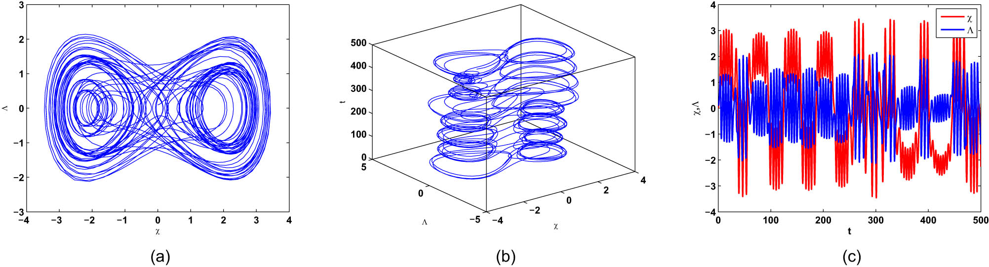
(a) 2D phase portrait, (b) 3D phase portrait, and (c) time-dependent waveforms of (50) with external force exhibit chaotic behavior for
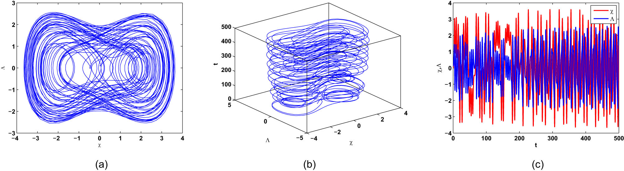
(a) 2D phase portrait, (b) 3D phase portrait, and (c) time-dependent waveforms of (50) with external force exhibit chaotic behavior for
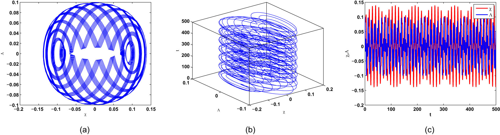
(a) 2D phase portrait, (b) 3D phase portrait, and (c) time-dependent waveforms of (50) with external force exhibit chaotic behavior for

(a) 2D phase portrait, (b) 3D phase portrait, and (c) time-dependent waveforms of (50) with external force exhibit chaotic behavior for
5 Graphical results
In this section, some interesting graphical plots of selected explicit exact solutions of (2), derived via the
5.1 Solution graphs generated using the
(
G
′
∕
G
,
1
∕
G
)
-expansion technique
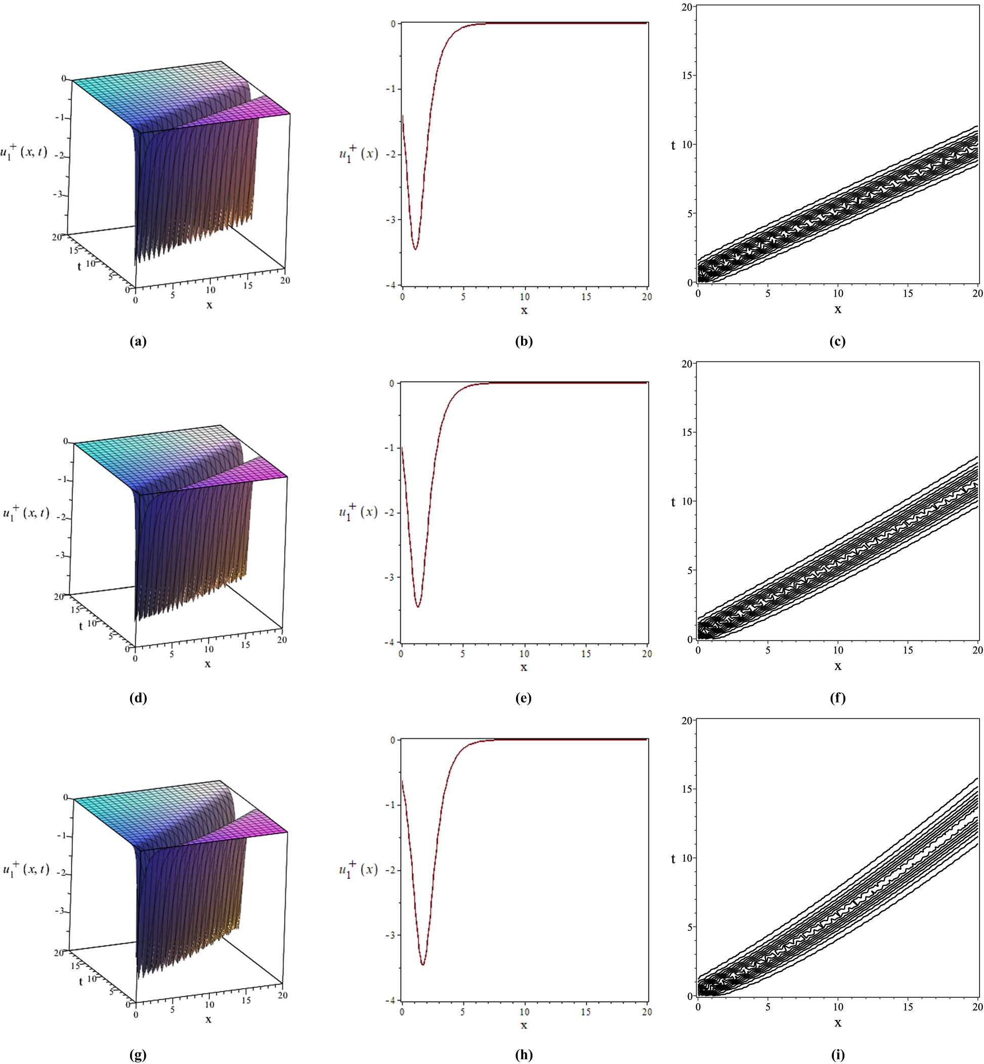
In this section, we show plots obtained from the
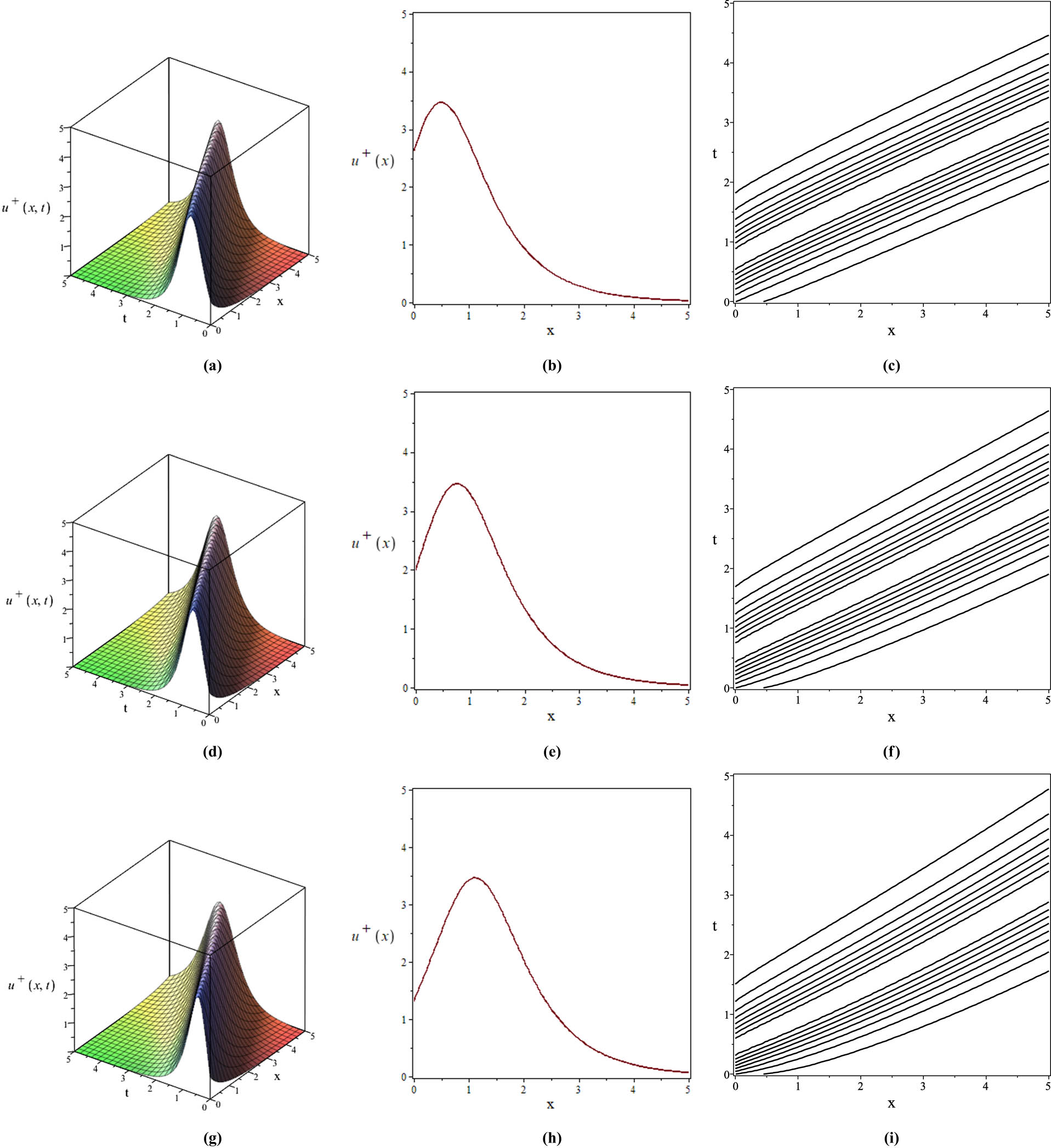
Graphs for
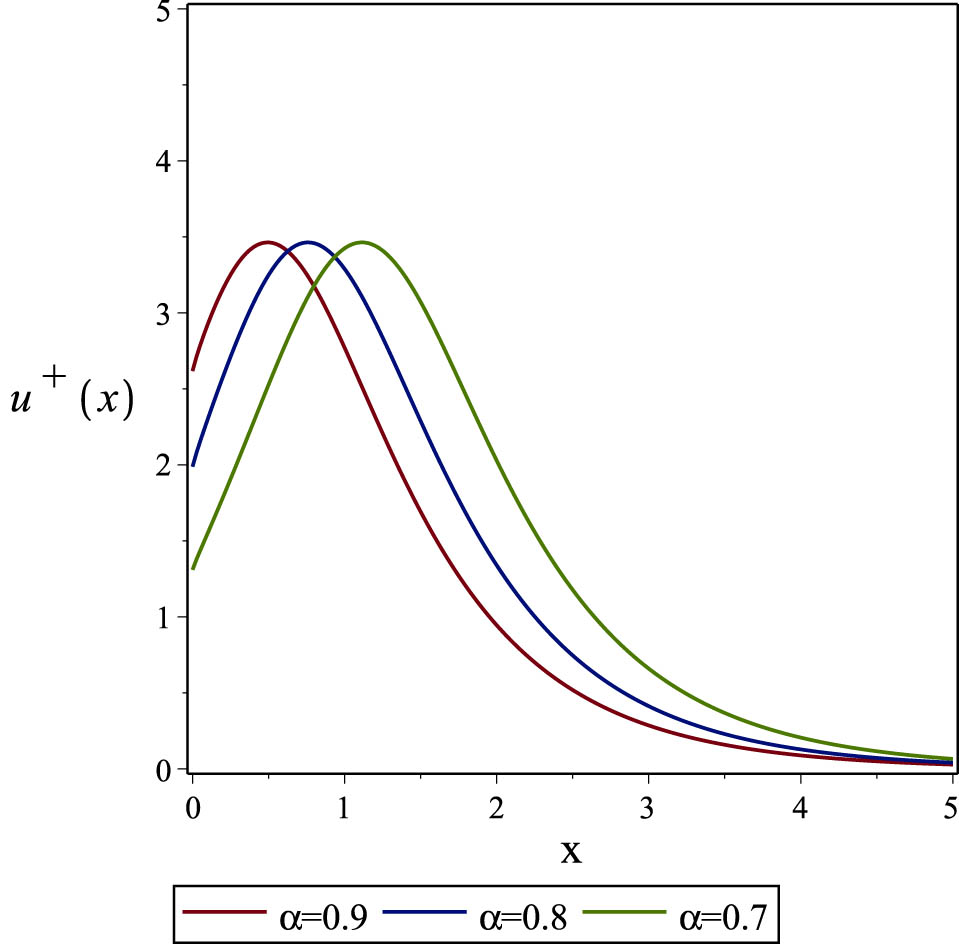
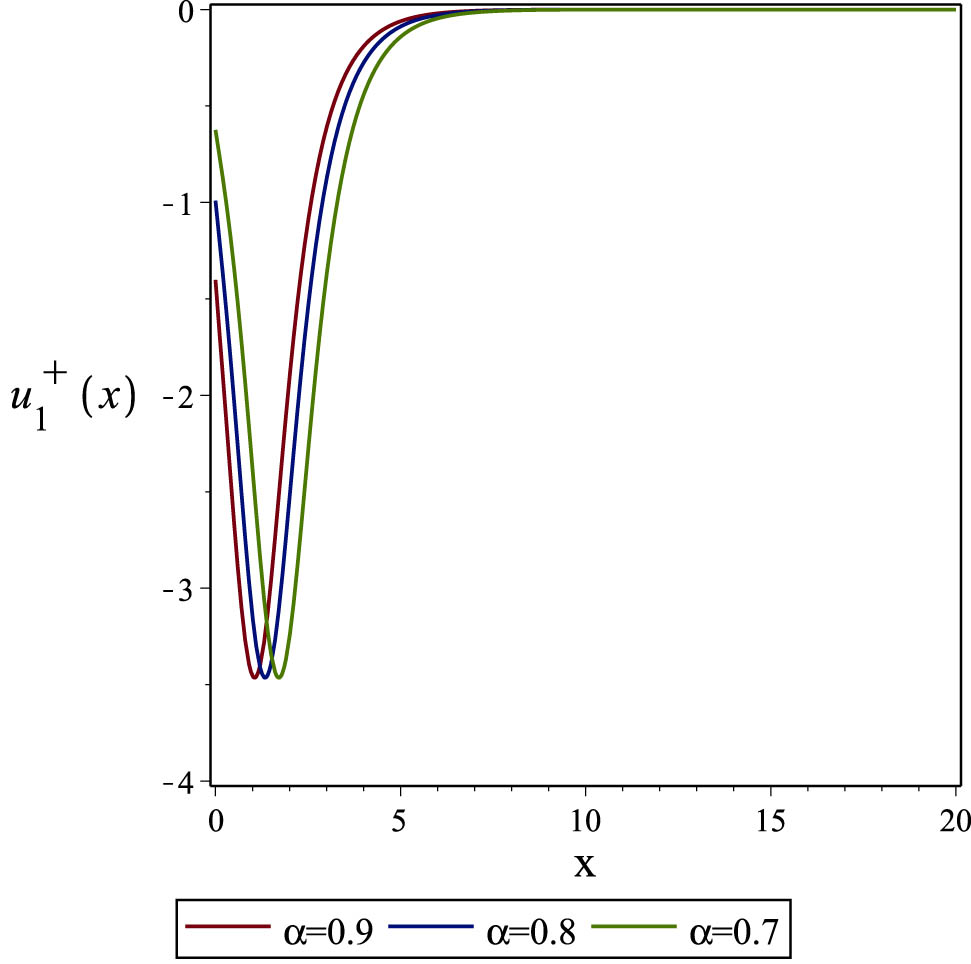
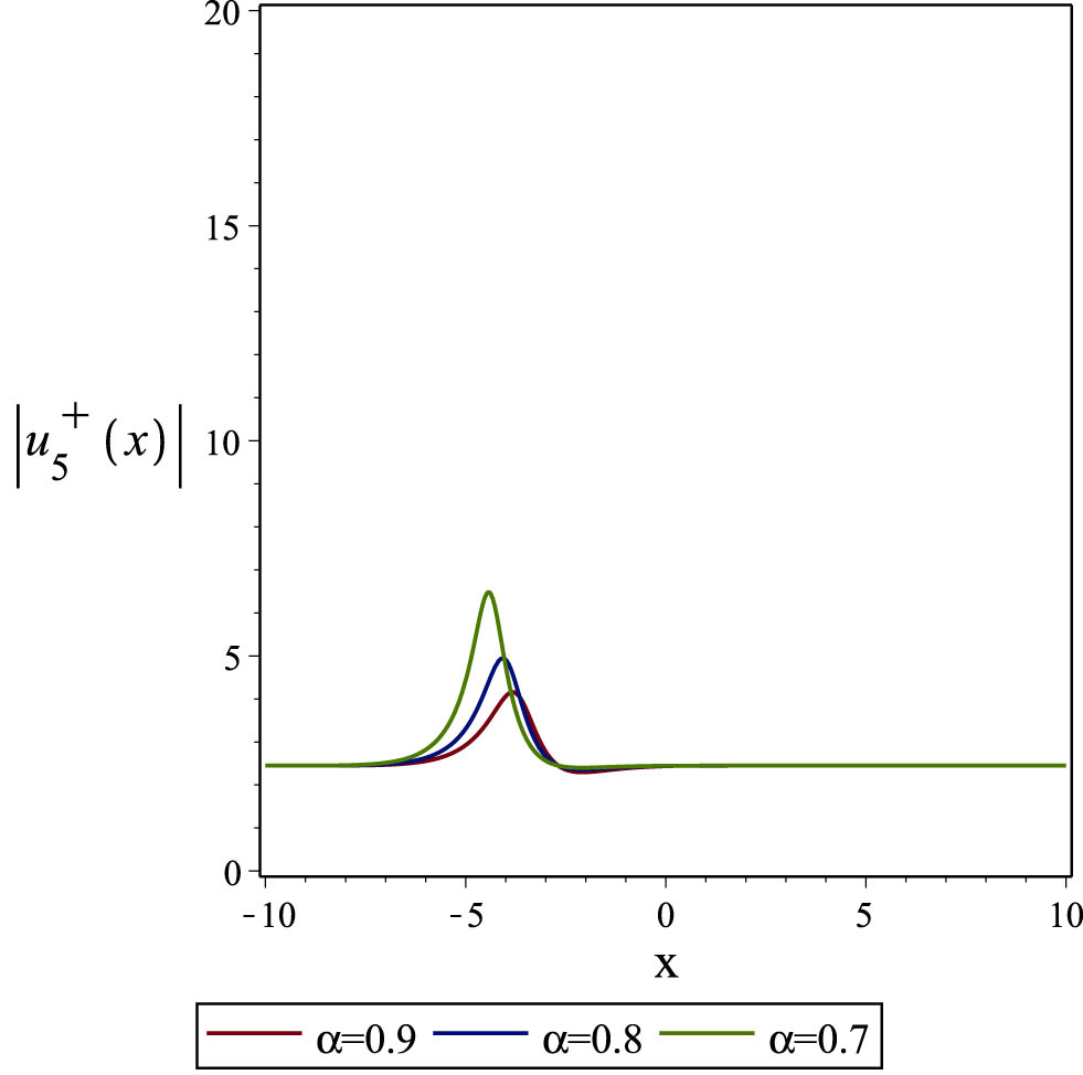
Effect of the time-fractional order
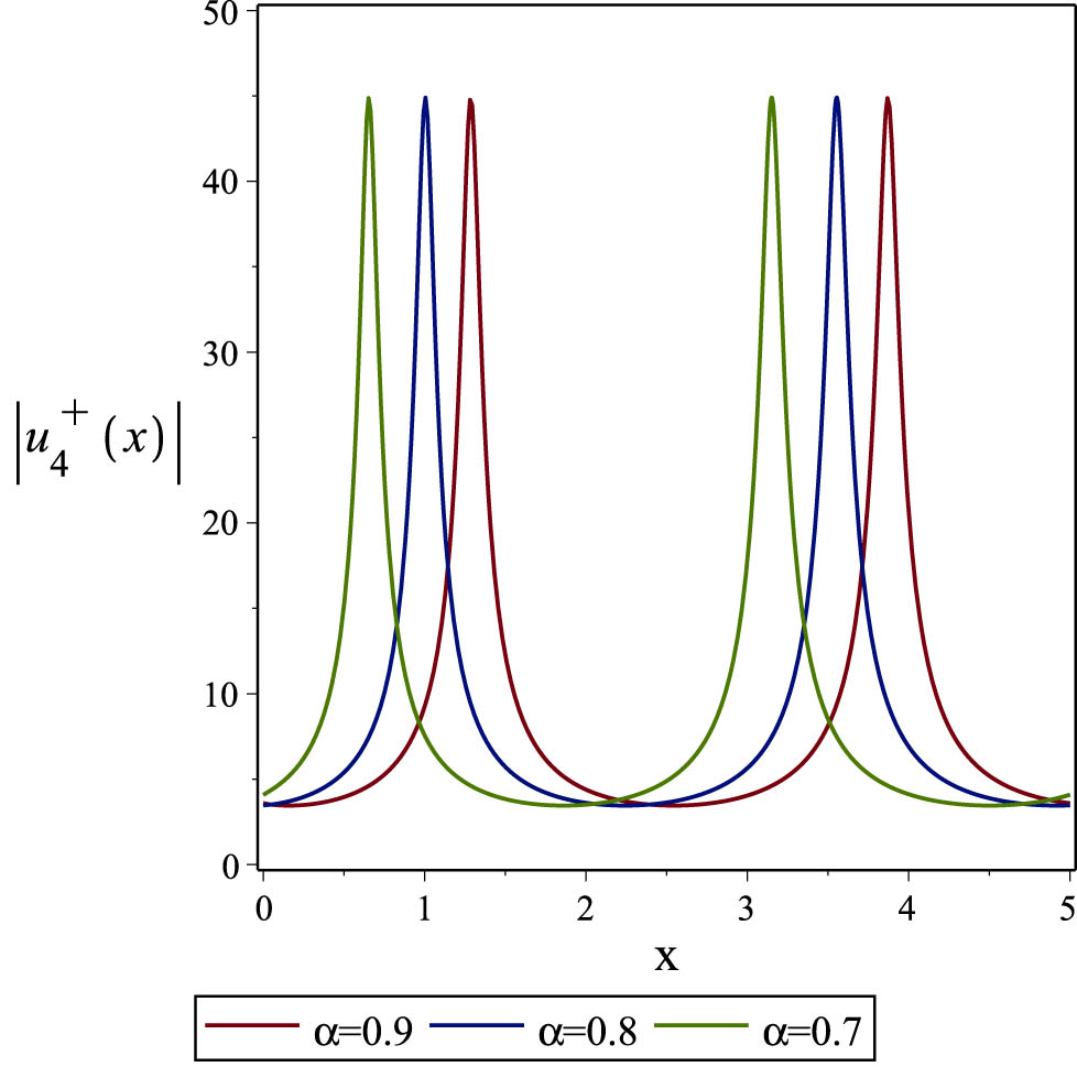
Figure 8 shows the magnitudes of
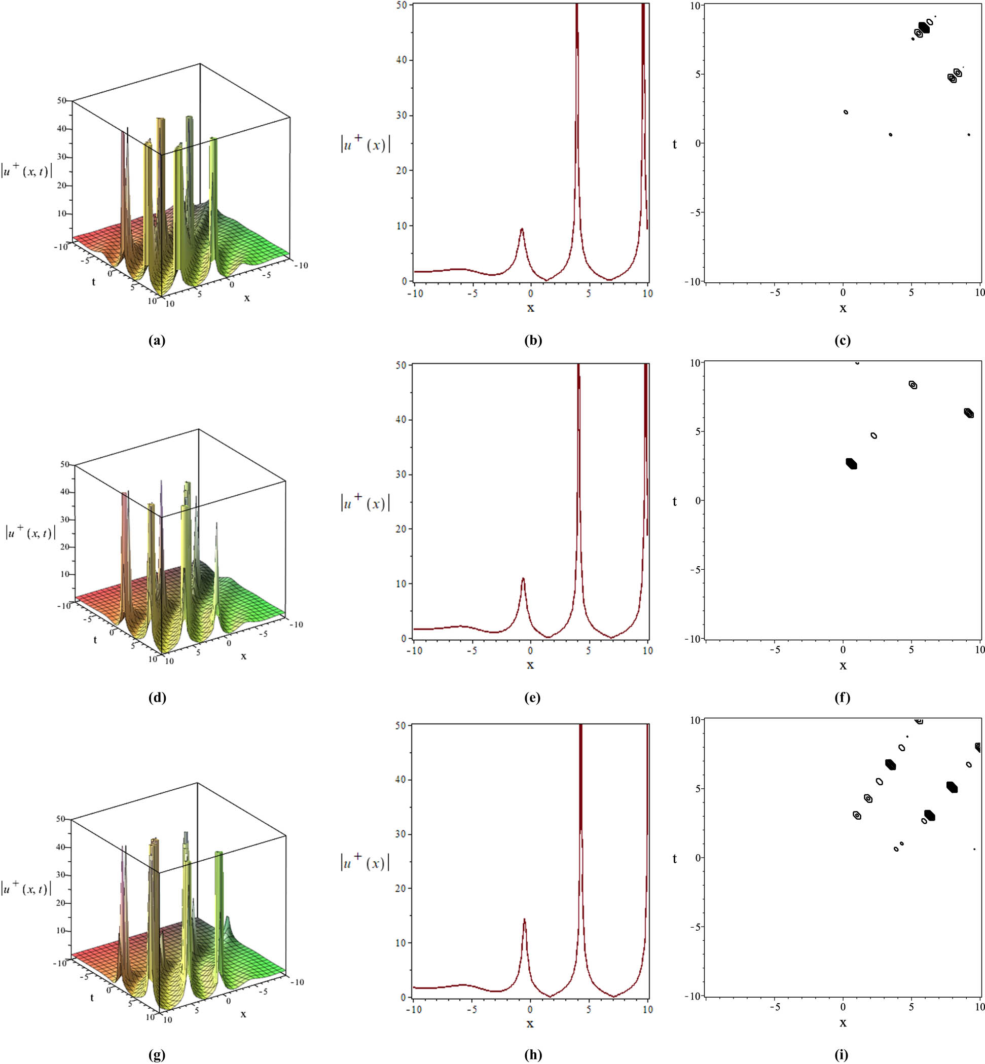
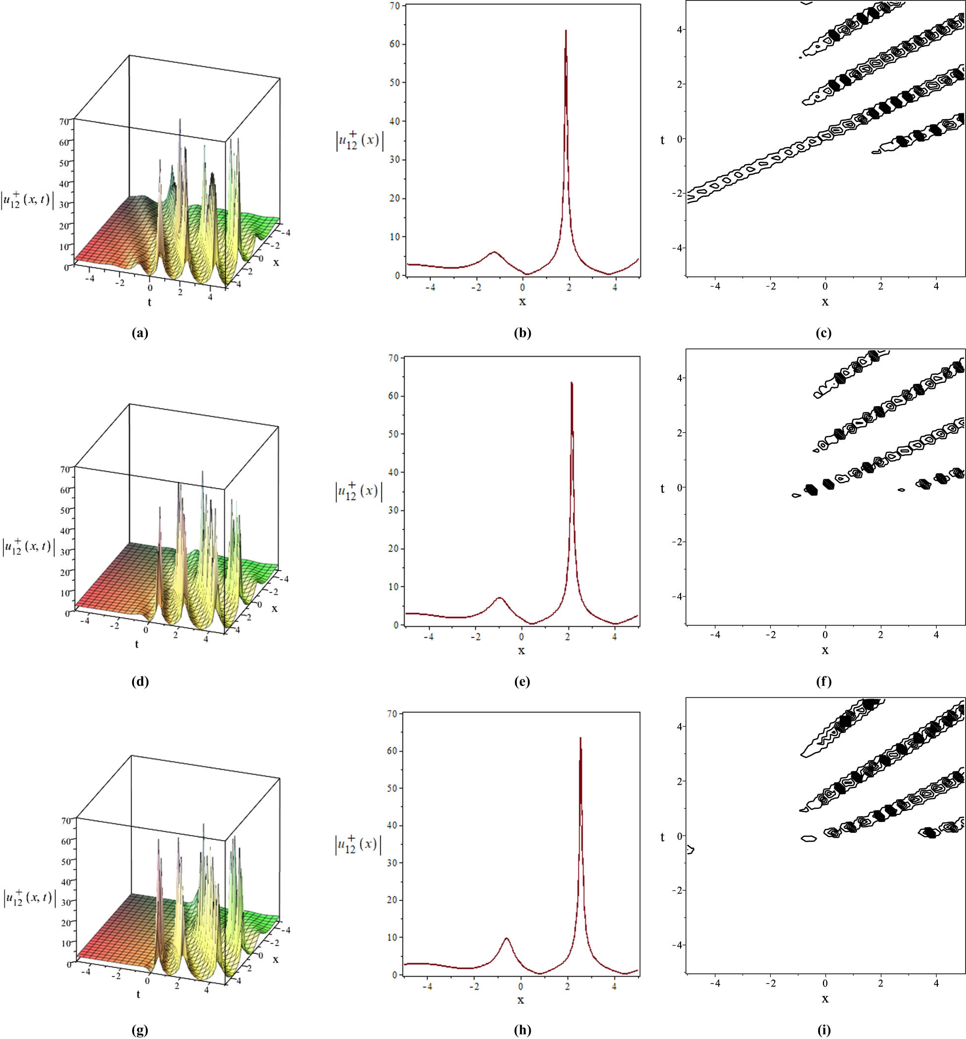
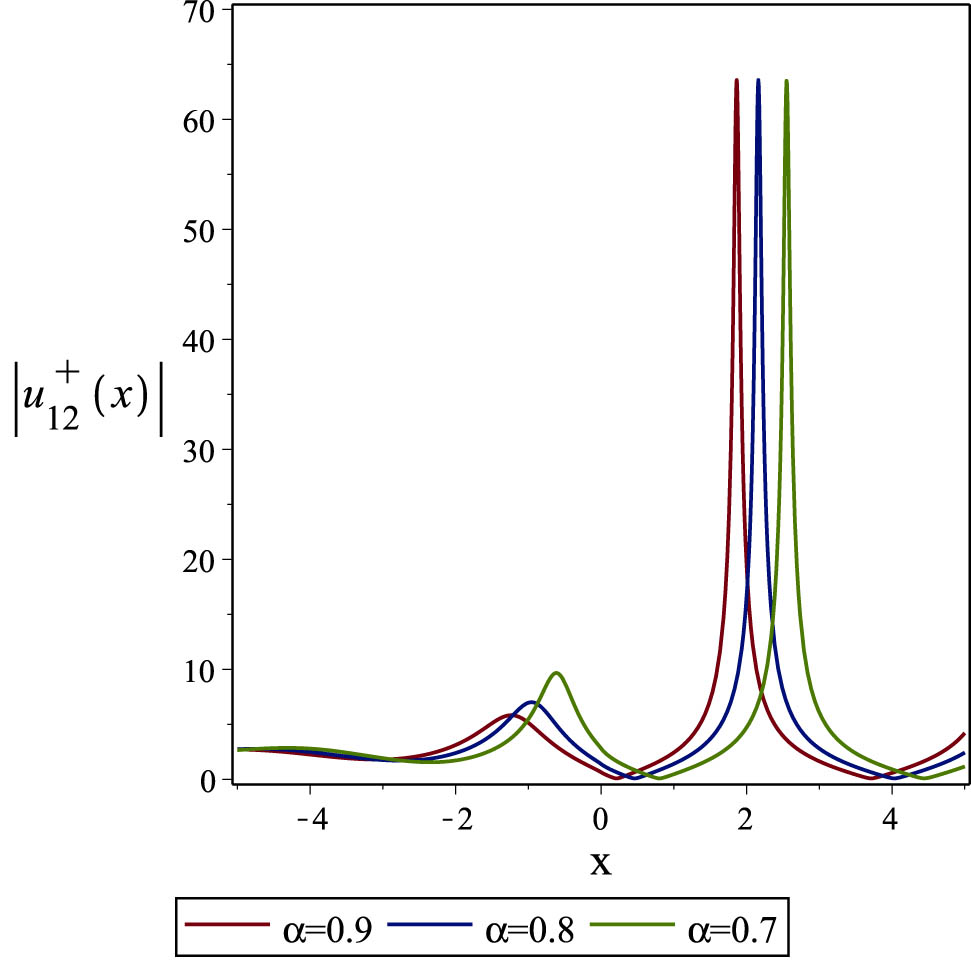
Graphs for the magnitude of
Effect of the time-fractional order
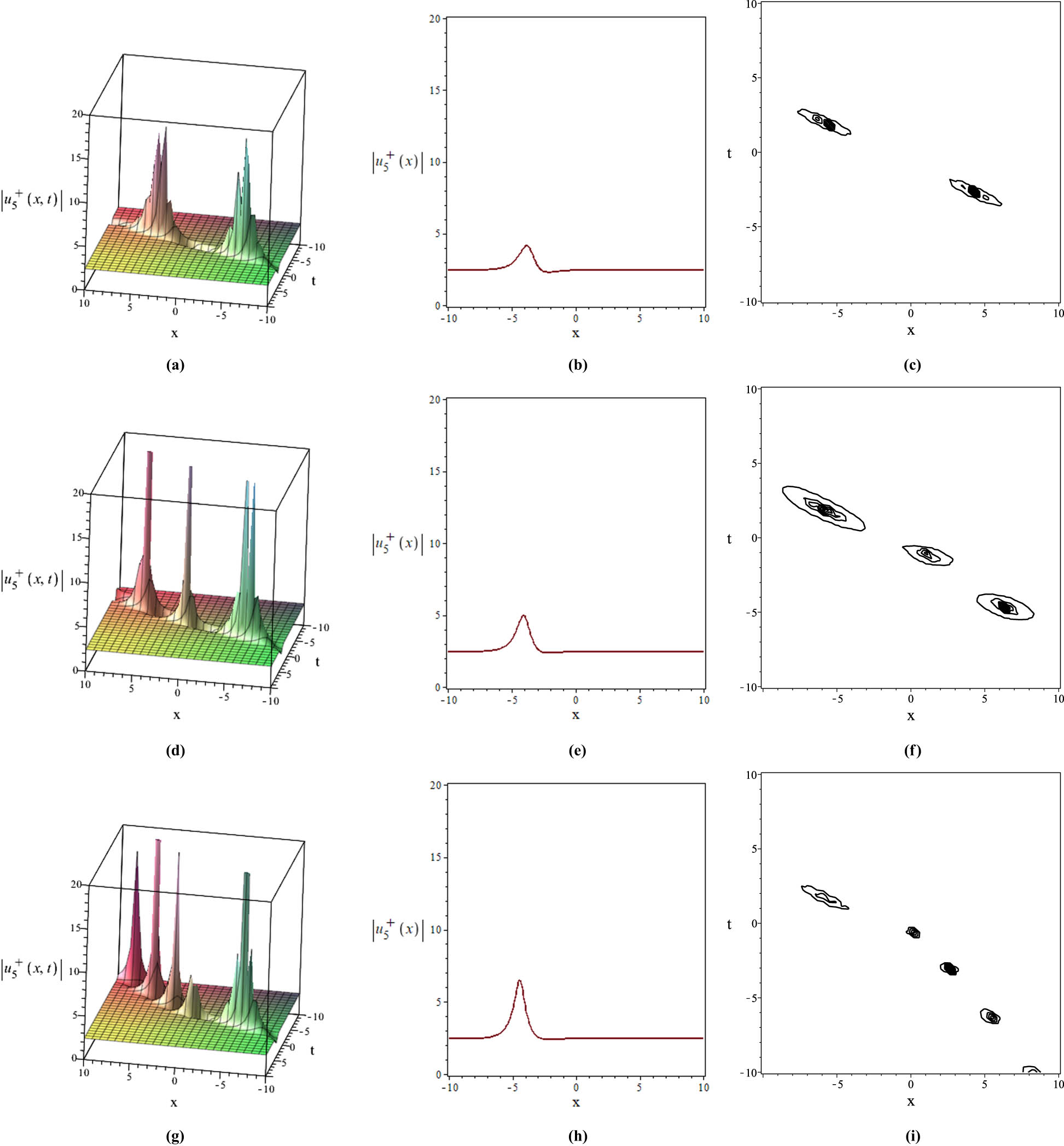
5.2 Solution graphs generated using the Sardar subequation scheme
In this section, the results from (2) derived by the Sardar subequation method are plotted for selected solutions, namely,
Graphs for
Effect of the time-fractional order
Magnitudes of

Graphs for
Effect of the time-fractional order
Magnitudes of
Graphs for
Effect of the time-fractional order
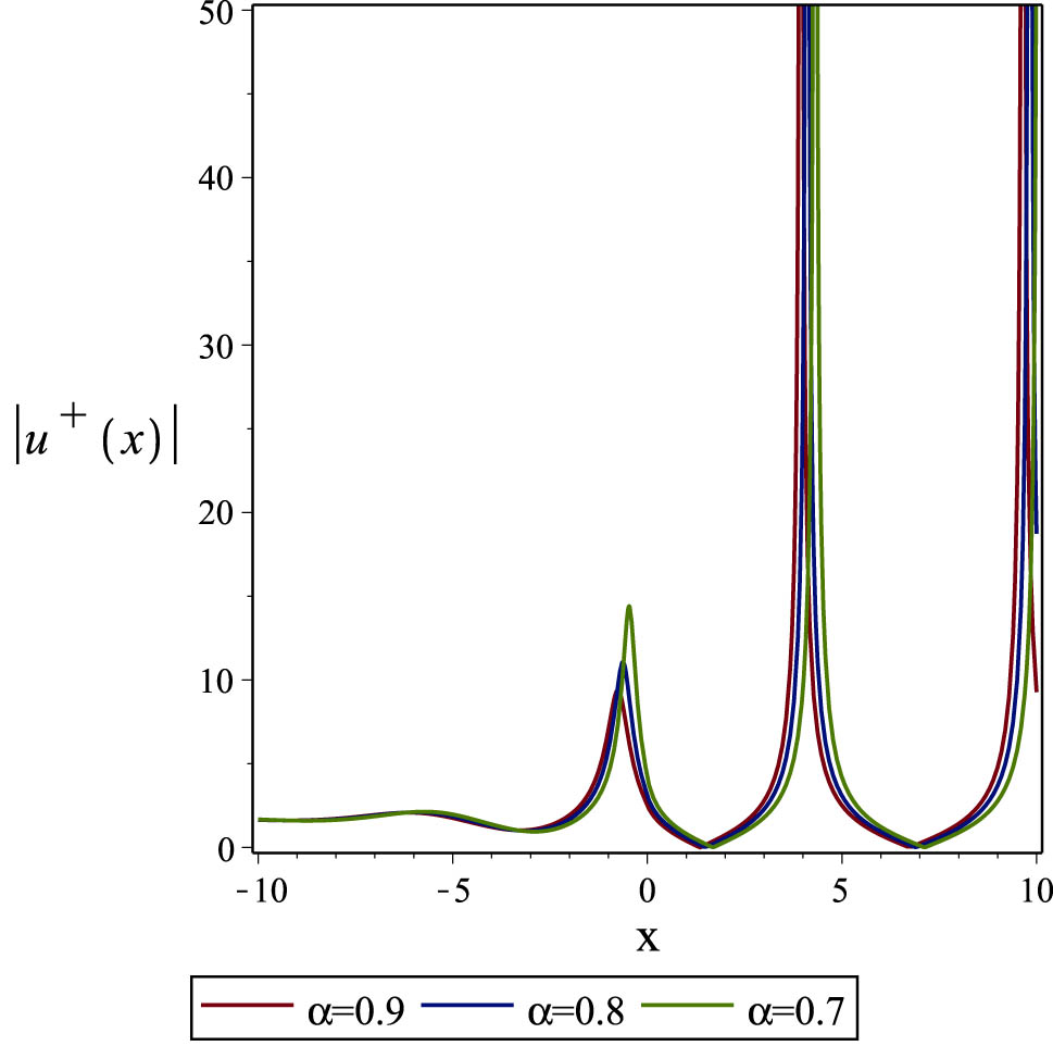
In Figure 16, magnitudes of
Graphs for
Effect of the time-fractional order
From all graphs shown previously, it can be seen that varying the fractional orders
6 Discussion and conclusions
The major findings of this article are to obtain a variety of novel exact traveling wave solutions of (2) via the
With the aid of Maple 17, all of the obtained exact solutions have been checked by substituting them back in the original problem. According to the results reported here, we have shown that both of the methods used here along with the aid of symbolic software such as Maple are fruitful, efficient, and reliable mathematical methods for generating exact traveling wave solutions of NPDEs. It has been recommended in future that the
-
Funding information: The authors greatly appreciate referees for their many significant comments and valuable suggestions. Sekson Sirisubtawee was supported by the Faculty of Applied Science, King Mongkut s University of Technology North Bangkok (Grant No. 672168).
-
Author contributions: Conceptualization of this study, P.W., S.S.; methodology, P.M., P.W.; formal analysis, P.W., S.S.; investigation, P.M., P.W., S.S.; software, P.W., S.S.; visualization, P.M., P.W., S.S.; validation, P.W., S.S.; data curation, S.S.; writing–original draft preparation, P.M., P.W., S.S.; writing–review and editing, P.M., P.W., S.S.; supervision project administration, S.S.; funding acquisition, S.S. All authors have accepted responsibility for the entire content of this manuscript and approved its submission.
-
Conflict of interest: The authors state no conflict of interest.
-
Data availability statement: All data generated or analysed during this study are included in this published article.
References
[1] Torvattanabun M, Khansai N, Sirisubtawee S, Koonprasert S, Tuan NM. New exact traveling wave solutions of the (3.1)-dimensional Chiral nonlinear Schrödinger equation using two reliable techniques. Thai J Math. 2024;22(1):145–63. Search in Google Scholar
[2] Tuan NM, Kooprasert S, Sirisubtawee S, Meesad P. The bilinear neural network method for solving Benney-Luke equation. Partial Differ Equ Appl Math. 2024;10:100682. 10.1016/j.padiff.2024.100682Search in Google Scholar
[3] Boakye G, Hosseini K, Hincccal E, Sirisubtawee S, Osman M. Some models of solitary wave propagation in optical fibers involving Kerr and parabolic laws. Optical Quantum Electronics. 2024;56(3):345. 10.1007/s11082-023-05903-5Search in Google Scholar
[4] Alqudah M, Shah SZH, Riaz MB, Khalifa HAEW, Akgül A, Ayub A. Neural network architecture to optimize the nanoscale thermal transport of ternary magnetized Carreau nanofluid over 3D wedge. Results Phys. 2024;59:107616. 10.1016/j.rinp.2024.107616Search in Google Scholar
[5] Manukure S, Booker T. A short overview of solitons and applications. Partial Differ Equ Appl Math. 2021;4: 100140. 10.1016/j.padiff.2021.100140Search in Google Scholar
[6] Sabíu J, Sirisubtawee S, Inc M. Optical soliton solutions for the Chavy-Waddy-Kolokolnikov model for bacterial colonies using two improved methods. J Appl Math Comput. 2024;70:1–24. 10.1007/s12190-024-02169-2Search in Google Scholar
[7] Rezazadeh H. New solitons solutions of the complex Ginzburg-Landau equation with Kerr law nonlinearity. Optik. 2018;167:218–27. 10.1016/j.ijleo.2018.04.026Search in Google Scholar
[8] Akbar MA, Akinyemi L, Yao SW, Jhangeer A, Rezazadeh H, Khater MM, et al. Soliton solutions to the Boussinesq equation through sine-Gordon method and Kudryashov method. Results Phys. 2021;25: 104228. 10.1016/j.rinp.2021.104228Search in Google Scholar
[9] León-Ramírez A, González-Gaxiola O, Chacón-Acosta G. Analytical solutions to the Chavy-Waddy-Kolokolnikov model of bacterial aggregates in phototaxis by three integration schemes. Mathematics. 2023;11(10):2352. 10.3390/math11102352Search in Google Scholar
[10] Sirisubtawee S, Koonprasert S, Sungnul S. Some applications of the (G′∕G,1∕G)-expansion method for finding exact traveling wave solutions of nonlinear fractional evolution equations. Symmetry. 2019;11(8):952. 10.3390/sym11080952Search in Google Scholar
[11] Pleumpreedaporn C, Pleumpreedaporn S, Moore EJ, Sirisubtawee S, Sungnul S. Novel exact traveling wave solutions for the (2+1)-dimensional Boiti-Leon-Manna-Pempinelli equation with Atangana’s space and time beta-derivatives via the Sardar subequation method: Annual Meeting in Mathematics 2023. Thai J Math. 2024;22(1):1–18. Search in Google Scholar
[12] Zakharov V, Kuznetsov EA. Three-dimensional solutions. Soviet Phys Uspekhi. 1974 Jan;39:285–6. Search in Google Scholar
[13] Kadomstev BB, Petviashvilli VI. On the stability of solitary waves in weakly dispersing media. Soviet Phys Doklady. 1970;15:539. Search in Google Scholar
[14] Mushtaq A, Shah H. Nonlinear Zakharov-Kuznetsov equation for obliquely propagating two-dimensional ion-acoustic solitary waves in a relativistic, rotating magnetized electron-positron-ion plasma. Phys Plasmas. 2005;12(7):072306. 10.1063/1.1946729Search in Google Scholar
[15] Biswas A, Zerrad E. Solitary wave solution of the Zakharov-Kuznetsov equation in plasmas with power law nonlinearity. Nonl Anal Real World Appl. 2010;11(4):3272–4. 10.1016/j.nonrwa.2009.08.007Search in Google Scholar
[16] Ray SS, Sahoo S. New exact solutions of fractional Zakharov-Kuznetsov and modified Zakharov-Kuznetsov equations using fractional sub-equation method. Commun Theoret Phys. 2015;63(1):25. 10.1088/0253-6102/63/1/05Search in Google Scholar
[17] Al-Amin M, Islam MN, Ilhan OA, Akbar MA, Soybaş D, et al. Solitary wave solutions to the modified Zakharov-Kuznetsov and the (2+1)-dimensional Calogero-Bogoyavlenskii-Schiff models in mathematical physics. J Math. 2022;2022(1):5224289. 10.1155/2022/5224289Search in Google Scholar
[18] Afrin FU. Solitary wave solutions and investigation the effects of different wave velocities of the nonlinear modified Zakharov-Kuznetsov model for the wave propagation in nonlinear media. Partial Differ Equ Appl Math. 2023;8:100583. 10.1016/j.padiff.2023.100583Search in Google Scholar
[19] Alam MN, Tunccc C. Constructions of the optical solitons and other solitons to the conformable fractional Zakharov-Kuznetsov equation with power law nonlinearity. J Taibah Univ Sci. 2020;14(1):94–100. 10.1080/16583655.2019.1708542Search in Google Scholar
[20] Munro S, Parkes E. The derivation of a modified Zakharov-Kuznetsov equation and the stability of its solutions. J Plasma Phys. 1999;62(3):305–17. 10.1017/S0022377899007874Search in Google Scholar
[21] Munro S, Parkes E. Stability of solitary-wave solutions to a modified Zakharov-Kuznetsov equation. J Plasma Phys. 2000;64(4):411–26. 10.1017/S0022377800008771Search in Google Scholar
[22] Zhang XZ, Siddique I, Mehdi KB, Elmandouh A, Inc M. Novel exact solutions, bifurcation of nonlinear and supernonlinear traveling waves for M-fractional generalized reaction Duffing model and the density dependent M-fractional diffusion reaction equation. Results Phys. 2022;37:105485. 10.1016/j.rinp.2022.105485Search in Google Scholar
[23] Siddique I, Mehdi KB, Jaradat MM, Zafar A, Elbrolosy ME, Elmandouh AA, et al. Bifurcation of some new traveling wave solutions for the time-space M-fractional MEW equation via three altered methods. Results Phys. 2022;41:105896. 10.1016/j.rinp.2022.105896Search in Google Scholar
[24] Han T, Zhang K, Jiang Y, Rezazadeh H. Chaotic pattern and solitary solutions for the (2+1)-dimensional beta-fractional double-chain DNA system. Fractal Fractional. 2024;8(7):415. 10.3390/fractalfract8070415Search in Google Scholar
[25] Mehdi KB, Mehdi Z, Samreen S, Siddique I, Elmandouh AA, Elbrolosy ME, et al. Novel exact traveling wave solutions of the space-time fractional Sharma Tasso-Olver equation via three reliable methods. Partial Differ Equ Appl Math. 2024;11:100784. 10.1016/j.padiff.2024.100784Search in Google Scholar
[26] Siddique I, Jaradat M, Zafar A, Mehdi KB, Osman M. Exact traveling wave solutions for two prolific conformable M-Fractional differential equations via three diverse approaches. Results Phys. 2021;28:104557. 10.1016/j.rinp.2021.104557Search in Google Scholar
[27] Guo M, Dong H, Liu J, Yang H. The time-fractional mZK equation for gravity solitary waves and solutions using sech-tanh and radial basic function method. Nonl Anal Model Control. 2019;24(1):1–19. 10.15388/NA.2019.1.1Search in Google Scholar
[28] Bibi A, Shakeel M, Khan D, Hussain S, Chou D. Study of solitary and kink waves, stability analysis, and fractional effect in magnetized plasma. Results Phys. 2023;44:106166. 10.1016/j.rinp.2022.106166Search in Google Scholar
[29] Fu L, Chen Y, Yang H. Time-space fractional coupled generalized Zakharov-Kuznetsov equations set for rossby solitary waves in two-layer fluids. Mathematics. 2019;7(1):41. 10.3390/math7010041Search in Google Scholar
[30] Baleanu D, Inç M, Yusuf A, Aliyu AI. Lie symmetry analysis, exact solutions and conservation laws for the time fractional modified Zakharov-Kuznetsov equation. Nonlinear Anal Model Control. 2017;22(6):861–76. 10.15388/NA.2017.6.9Search in Google Scholar
[31] Gorenflo R, Kilbas AA, Mainardi F, Rogosin SV. Mittag-Leffler functions, related topics and applications. Berlin: Springer; 2020. 10.1007/978-3-662-61550-8Search in Google Scholar
[32] Mittag-Leffler GM. Sur la nouvelle fonction Ealpha(x). CR Acad Sci Paris. 1903;137(2):554–8. Search in Google Scholar
[33] Sousa J, de Oliveira EC. A new truncated M-fractional derivative type unifying some fractional derivative types with classical properties. Int J Anal Appl. 2018;16(1):83–96. Search in Google Scholar
[34] Riaz MB, Awrejcewicz J, Jhangeer A. Optical solitons with beta and M-truncated derivatives in nonlinear negative-index materials with Bohm potential. Materials. 2021;14(18):5335. 10.3390/ma14185335Search in Google Scholar PubMed PubMed Central
[35] Yao SW, Manzoor R, Zafar A, Inc M, Abbagari S, Houwe A. Exact soliton solutions to the Cahn-Allen equation and Predator-Prey model with truncated M-fractional derivative. Results Phys. 2022;37:105455. 10.1016/j.rinp.2022.105455Search in Google Scholar
[36] Chauhan RB, Chudasama MH. A study of the left local general truncated M-fractional derivative. Appl Math E-Notes. 2023;23:100–23. Search in Google Scholar
[37] Onder I, Cinar M, Secer A, Bayram M. Analytical solutions of simplified modified Camassa-Holm equation with conformable and M-truncated derivatives: A comparative study. J Ocean Eng Sci. 2024;9(3):240–50. 10.1016/j.joes.2022.06.012Search in Google Scholar
[38] Raheel M, Razzaq W, Alsharidi AK, Zafar A. Exact solitons to M-fractional (2.1)-dimensional CNLSE based on three different methods. Results Phys. 2022;42:105983. 10.1016/j.rinp.2022.105983Search in Google Scholar
[39] Mohammed WW, Cesarano C, Al-Askar FM. Solutions to the (4+1)-dimensional time-fractional Fokas equation with M-truncated derivative. Mathematics. 2022;11(1):194. 10.3390/math11010194Search in Google Scholar
[40] Roshid HO, Roshid MM, Hossain MM, Hasan MS, Munshi MJH, Sajib AH. Dynamical structure of truncated M- fractional Klein-Gordon model via two integral schemes. Results Phys. 2023;46:106272. 10.1016/j.rinp.2023.106272Search in Google Scholar
[41] Ozdemir N. M-truncated soliton solutions of the fractional (4+1)-dimensional Fokas equation. Int J Optimiz Control Theories Appl (IJOCTA). 2023;13(1):123–9. 10.11121/ijocta.2023.1321Search in Google Scholar
[42] Malingam P, Wongsasinchai P, Sirisubtawee S, Koonprasert S. Exact solutions of the paraxial wave dynamical model in Kerr media with truncated M-fractional derivative using the (G′∕G,1∕G)-expansion method. WSEAS Trans Syst Control. 2023;18:498–512. 10.37394/23203.2023.18.53Search in Google Scholar
[43] Khalil R, Al Horani M, Yousef A, Sababheh M. A new definition of fractional derivative. J Comput Appl Math. 2014;264:65–70. 10.1016/j.cam.2014.01.002Search in Google Scholar
[44] Katugampola UN. A new fractional derivative with classical properties. Classical Analysis and ODEs. 2014;1–8. https://arxiv.org/abs/1410.6535. Search in Google Scholar
[45] Demiray S, Ünsal Ö, Bekir A. Exact solutions of nonlinear wave equations using (G′G,1G)-expansion method. J Egypt Math Soc. 2015;23(1):78–84. 10.1016/j.joems.2014.02.011Search in Google Scholar
[46] Miah MM, Ali HS, Akbar MA, Seadawy AR. New applications of the two variable (G′∕G,1∕G)-expansion method for closed form traveling wave solutions of integro-differential equations. J Ocean Eng Sci. 2019;4(2):132–43. 10.1016/j.joes.2019.03.001Search in Google Scholar
[47] Alurrfi KA, Shahoot AM, Elhasadi OI. Exact solutions for the GKdV-mKdV equation with higher-order nonlinear terms using the generalized (G′∕G,1∕G)-expansion method and the generalized Liénardequation. Ricerche di Matematica. 2024;73:887–905. 10.1007/s11587-021-00637-6Search in Google Scholar
[48] Sadaf M, Arshed S, Akram G, Iqra. Exact soliton and solitary wave solutions to the Fokas system using two variables (G′∕G,1∕G)-expansion technique and generalized projective Riccati equation method. Optik. 2022;268:169713. 10.1016/j.ijleo.2022.169713Search in Google Scholar
[49] Ahmad S, Mahmoud EE, Saifullah S, Ullah A, Ahmad S, Akgül A, et al. New waves solutions of a nonlinear Landau-Ginzburg-Higgs equation: The Sardar-subequation and energy balance approaches. Results Phys. 2023;51:106736. 10.1016/j.rinp.2023.106736Search in Google Scholar
[50] Hussain R, Imtiaz A, Rasool T, Rezazadeh H, Inç M. Novel exact and solitary solutions of conformable Klein-Gordon equation via Sardar-subequation method. J Ocean Eng Sci. 2022;7(1):1–7. 10.1016/j.joes.2022.04.036Search in Google Scholar
[51] Asjad MI, Inc M, Iqbal I. Exact solutions for new coupled Konno-Oono equation via Sardar subequation method. Optical Quantum Electron. 2022;54(12):798. 10.1007/s11082-022-04208-3Search in Google Scholar
[52] Rezazadeh H, Inc M, Baleanu D. New solitary wave solutions for variants of (3+1)-dimensional Wazwaz-Benjamin-Bona-Mahony equations. Front Phys. 2020;8:332. 10.3389/fphy.2020.00332Search in Google Scholar
[53] Tang L. Bifurcation analysis and optical soliton solutions for the fractional complex Ginzburg-Landau equation in communication systems. Optik. 2023;276:170639. 10.1016/j.ijleo.2023.170639Search in Google Scholar
[54] Nguetcho AT, Li J, Bilbault JM. Bifurcations of phase portraits of a singular nonlinear equation of the second class. Commun Nonl Sci Numer Simul. 2014;19(8):2590–601. 10.1016/j.cnsns.2013.12.022Search in Google Scholar
[55] Ali KK, Mehanna M. Computational and analytical solutions to modified Zakharov-Kuznetsov model with stability analysis via efficient techniques. Opt Quantum Electron. 2021;53(12):723. 10.1007/s11082-021-03363-3Search in Google Scholar
[56] Zayed E, Alurrfi K. The (G′∕G,1∕G)-expansion method and its applications to two nonlinear Schrödinger equations describing the propagation of femtosecond pulses in nonlinear optical fibers. Optik. 2016;127(4):1581–89. 10.1016/j.ijleo.2015.11.027Search in Google Scholar
© 2025 the author(s), published by De Gruyter
This work is licensed under the Creative Commons Attribution 4.0 International License.
Articles in the same Issue
- Research Articles
- Single-step fabrication of Ag2S/poly-2-mercaptoaniline nanoribbon photocathodes for green hydrogen generation from artificial and natural red-sea water
- Abundant new interaction solutions and nonlinear dynamics for the (3+1)-dimensional Hirota–Satsuma–Ito-like equation
- A novel gold and SiO2 material based planar 5-element high HPBW end-fire antenna array for 300 GHz applications
- Explicit exact solutions and bifurcation analysis for the mZK equation with truncated M-fractional derivatives utilizing two reliable methods
- Optical and laser damage resistance: Role of periodic cylindrical surfaces
- Numerical study of flow and heat transfer in the air-side metal foam partially filled channels of panel-type radiator under forced convection
- Water-based hybrid nanofluid flow containing CNT nanoparticles over an extending surface with velocity slips, thermal convective, and zero-mass flux conditions
- Dynamical wave structures for some diffusion--reaction equations with quadratic and quartic nonlinearities
- Solving an isotropic grey matter tumour model via a heat transfer equation
- Study on the penetration protection of a fiber-reinforced composite structure with CNTs/GFP clip STF/3DKevlar
- Influence of Hall current and acoustic pressure on nanostructured DPL thermoelastic plates under ramp heating in a double-temperature model
- Applications of the Belousov–Zhabotinsky reaction–diffusion system: Analytical and numerical approaches
- AC electroosmotic flow of Maxwell fluid in a pH-regulated parallel-plate silica nanochannel
- Interpreting optical effects with relativistic transformations adopting one-way synchronization to conserve simultaneity and space–time continuity
- Modeling and analysis of quantum communication channel in airborne platforms with boundary layer effects
- Theoretical and numerical investigation of a memristor system with a piecewise memductance under fractal–fractional derivatives
- Tuning the structure and electro-optical properties of α-Cr2O3 films by heat treatment/La doping for optoelectronic applications
- High-speed multi-spectral explosion temperature measurement using golden-section accelerated Pearson correlation algorithm
- Dynamic behavior and modulation instability of the generalized coupled fractional nonlinear Helmholtz equation with cubic–quintic term
- Study on the duration of laser-induced air plasma flash near thin film surface
- Exploring the dynamics of fractional-order nonlinear dispersive wave system through homotopy technique
- The mechanism of carbon monoxide fluorescence inside a femtosecond laser-induced plasma
- Numerical solution of a nonconstant coefficient advection diffusion equation in an irregular domain and analyses of numerical dispersion and dissipation
- Numerical examination of the chemically reactive MHD flow of hybrid nanofluids over a two-dimensional stretching surface with the Cattaneo–Christov model and slip conditions
- Impacts of sinusoidal heat flux and embraced heated rectangular cavity on natural convection within a square enclosure partially filled with porous medium and Casson-hybrid nanofluid
- Stability analysis of unsteady ternary nanofluid flow past a stretching/shrinking wedge
- Solitonic wave solutions of a Hamiltonian nonlinear atom chain model through the Hirota bilinear transformation method
- Bilinear form and soltion solutions for (3+1)-dimensional negative-order KdV-CBS equation
- Solitary chirp pulses and soliton control for variable coefficients cubic–quintic nonlinear Schrödinger equation in nonuniform management system
- Influence of decaying heat source and temperature-dependent thermal conductivity on photo-hydro-elasto semiconductor media
- Dissipative disorder optimization in the radiative thin film flow of partially ionized non-Newtonian hybrid nanofluid with second-order slip condition
- Bifurcation, chaotic behavior, and traveling wave solutions for the fractional (4+1)-dimensional Davey–Stewartson–Kadomtsev–Petviashvili model
- New investigation on soliton solutions of two nonlinear PDEs in mathematical physics with a dynamical property: Bifurcation analysis
- Mathematical analysis of nanoparticle type and volume fraction on heat transfer efficiency of nanofluids
- Creation of single-wing Lorenz-like attractors via a ten-ninths-degree term
- Optical soliton solutions, bifurcation analysis, chaotic behaviors of nonlinear Schrödinger equation and modulation instability in optical fiber
- Chaotic dynamics and some solutions for the (n + 1)-dimensional modified Zakharov–Kuznetsov equation in plasma physics
- Fractal formation and chaotic soliton phenomena in nonlinear conformable Heisenberg ferromagnetic spin chain equation
- Single-step fabrication of Mn(iv) oxide-Mn(ii) sulfide/poly-2-mercaptoaniline porous network nanocomposite for pseudo-supercapacitors and charge storage
- Novel constructed dynamical analytical solutions and conserved quantities of the new (2+1)-dimensional KdV model describing acoustic wave propagation
- Tavis–Cummings model in the presence of a deformed field and time-dependent coupling
- Spinning dynamics of stress-dependent viscosity of generalized Cross-nonlinear materials affected by gravitationally swirling disk
- Design and prediction of high optical density photovoltaic polymers using machine learning-DFT studies
- Robust control and preservation of quantum steering, nonlocality, and coherence in open atomic systems
- Coating thickness and process efficiency of reverse roll coating using a magnetized hybrid nanomaterial flow
- Dynamic analysis, circuit realization, and its synchronization of a new chaotic hyperjerk system
- Decoherence of steerability and coherence dynamics induced by nonlinear qubit–cavity interactions
- Finite element analysis of turbulent thermal enhancement in grooved channels with flat- and plus-shaped fins
- Modulational instability and associated ion-acoustic modulated envelope solitons in a quantum plasma having ion beams
- Statistical inference of constant-stress partially accelerated life tests under type II generalized hybrid censored data from Burr III distribution
- On solutions of the Dirac equation for 1D hydrogenic atoms or ions
- Entropy optimization for chemically reactive magnetized unsteady thin film hybrid nanofluid flow on inclined surface subject to nonlinear mixed convection and variable temperature
- Stability analysis, circuit simulation, and color image encryption of a novel four-dimensional hyperchaotic model with hidden and self-excited attractors
- A high-accuracy exponential time integration scheme for the Darcy–Forchheimer Williamson fluid flow with temperature-dependent conductivity
- Novel analysis of fractional regularized long-wave equation in plasma dynamics
- Development of a photoelectrode based on a bismuth(iii) oxyiodide/intercalated iodide-poly(1H-pyrrole) rough spherical nanocomposite for green hydrogen generation
- Investigation of solar radiation effects on the energy performance of the (Al2O3–CuO–Cu)/H2O ternary nanofluidic system through a convectively heated cylinder
- Quantum resources for a system of two atoms interacting with a deformed field in the presence of intensity-dependent coupling
- Studying bifurcations and chaotic dynamics in the generalized hyperelastic-rod wave equation through Hamiltonian mechanics
- A new numerical technique for the solution of time-fractional nonlinear Klein–Gordon equation involving Atangana–Baleanu derivative using cubic B-spline functions
- Interaction solutions of high-order breathers and lumps for a (3+1)-dimensional conformable fractional potential-YTSF-like model
- Hydraulic fracturing radioactive source tracing technology based on hydraulic fracturing tracing mechanics model
- Numerical solution and stability analysis of non-Newtonian hybrid nanofluid flow subject to exponential heat source/sink over a Riga sheet
- Numerical investigation of mixed convection and viscous dissipation in couple stress nanofluid flow: A merged Adomian decomposition method and Mohand transform
- Effectual quintic B-spline functions for solving the time fractional coupled Boussinesq–Burgers equation arising in shallow water waves
- Analysis of MHD hybrid nanofluid flow over cone and wedge with exponential and thermal heat source and activation energy
- Solitons and travelling waves structure for M-fractional Kairat-II equation using three explicit methods
- Impact of nanoparticle shapes on the heat transfer properties of Cu and CuO nanofluids flowing over a stretching surface with slip effects: A computational study
- Computational simulation of heat transfer and nanofluid flow for two-sided lid-driven square cavity under the influence of magnetic field
- Irreversibility analysis of a bioconvective two-phase nanofluid in a Maxwell (non-Newtonian) flow induced by a rotating disk with thermal radiation
- Hydrodynamic and sensitivity analysis of a polymeric calendering process for non-Newtonian fluids with temperature-dependent viscosity
- Exploring the peakon solitons molecules and solitary wave structure to the nonlinear damped Kortewege–de Vries equation through efficient technique
- Modeling and heat transfer analysis of magnetized hybrid micropolar blood-based nanofluid flow in Darcy–Forchheimer porous stenosis narrow arteries
- Activation energy and cross-diffusion effects on 3D rotating nanofluid flow in a Darcy–Forchheimer porous medium with radiation and convective heating
- Insights into chemical reactions occurring in generalized nanomaterials due to spinning surface with melting constraints
- Influence of a magnetic field on double-porosity photo-thermoelastic materials under Lord–Shulman theory
- Soliton-like solutions for a nonlinear doubly dispersive equation in an elastic Murnaghan's rod via Hirota's bilinear method
- Analytical and numerical investigation of exact wave patterns and chaotic dynamics in the extended improved Boussinesq equation
- Nonclassical correlation dynamics of Heisenberg XYZ states with (x, y)-spin--orbit interaction, x-magnetic field, and intrinsic decoherence effects
- Exact traveling wave and soliton solutions for chemotaxis model and (3+1)-dimensional Boiti–Leon–Manna–Pempinelli equation
- Unveiling the transformative role of samarium in ZnO: Exploring structural and optical modifications for advanced functional applications
- On the derivation of solitary wave solutions for the time-fractional Rosenau equation through two analytical techniques
- Analyzing the role of length and radius of MWCNTs in a nanofluid flow influenced by variable thermal conductivity and viscosity considering Marangoni convection
- Advanced mathematical analysis of heat and mass transfer in oscillatory micropolar bio-nanofluid flows via peristaltic waves and electroosmotic effects
- Exact bound state solutions of the radial Schrödinger equation for the Coulomb potential by conformable Nikiforov–Uvarov approach
- Some anisotropic and perfect fluid plane symmetric solutions of Einstein's field equations using killing symmetries
- Nonlinear dynamics of the dissipative ion-acoustic solitary waves in anisotropic rotating magnetoplasmas
- Curves in multiplicative equiaffine plane
- Exact solution of the three-dimensional (3D) Z2 lattice gauge theory
- Propagation properties of Airyprime pulses in relaxing nonlinear media
- Symbolic computation: Analytical solutions and dynamics of a shallow water wave equation in coastal engineering
- Wave propagation in nonlocal piezo-photo-hygrothermoelastic semiconductors subjected to heat and moisture flux
- Comparative reaction dynamics in rotating nanofluid systems: Quartic and cubic kinetics under MHD influence
- Laplace transform technique and probabilistic analysis-based hypothesis testing in medical and engineering applications
- Physical properties of ternary chloro-perovskites KTCl3 (T = Ge, Al) for optoelectronic applications
- Gravitational length stretching: Curvature-induced modulation of quantum probability densities
- The search for the cosmological cold dark matter axion – A new refined narrow mass window and detection scheme
- A comparative study of quantum resources in bipartite Lipkin–Meshkov–Glick model under DM interaction and Zeeman splitting
- PbO-doped K2O–BaO–Al2O3–B2O3–TeO2-glasses: Mechanical and shielding efficacy
- Nanospherical arsenic(iii) oxoiodide/iodide-intercalated poly(N-methylpyrrole) composite synthesis for broad-spectrum optical detection
- Sine power Burr X distribution with estimation and applications in physics and other fields
- Numerical modeling of enhanced reactive oxygen plasma in pulsed laser deposition of metal oxide thin films
- Dynamical analyses and dispersive soliton solutions to the nonlinear fractional model in stratified fluids
- Computation of exact analytical soliton solutions and their dynamics in advanced optical system
- An innovative approximation concerning the diffusion and electrical conductivity tensor at critical altitudes within the F-region of ionospheric plasma at low latitudes
- An analytical investigation to the (3+1)-dimensional Yu–Toda–Sassa–Fukuyama equation with dynamical analysis: Bifurcation
- Swirling-annular-flow-induced instability of a micro shell considering Knudsen number and viscosity effects
- Numerical analysis of non-similar convection flows of a two-phase nanofluid past a semi-infinite vertical plate with thermal radiation
- MgO NPs reinforced PCL/PVC nanocomposite films with enhanced UV shielding and thermal stability for packaging applications
- Optimal conditions for indoor air purification using non-thermal Corona discharge electrostatic precipitator
- Investigation of thermal conductivity and Raman spectra for HfAlB, TaAlB, and WAlB based on first-principles calculations
- Tunable double plasmon-induced transparency based on monolayer patterned graphene metamaterial
- DSC: depth data quality optimization framework for RGBD camouflaged object detection
- A new family of Poisson-exponential distributions with applications to cancer data and glass fiber reliability
- Numerical investigation of couple stress under slip conditions via modified Adomian decomposition method
- Monitoring plateau lake area changes in Yunnan province, southwestern China using medium-resolution remote sensing imagery: applicability of water indices and environmental dependencies
- Heterodyne interferometric fiber-optic gyroscope
- Exact solutions of Einstein’s field equations via homothetic symmetries of non-static plane symmetric spacetime
- A widespread study of discrete entropic model and its distribution along with fluctuations of energy
- Empirical model integration for accurate charge carrier mobility simulation in silicon MOSFETs
- The influence of scattering correction effect based on optical path distribution on CO2 retrieval
- Anisotropic dissociation and spectral response of 1-Bromo-4-chlorobenzene under static directional electric fields
- Role of tungsten oxide (WO3) on thermal and optical properties of smart polymer composites
- Analysis of iterative deblurring: no explicit noise
- The influence of anisotropy of InP on its elasticity and phonon properties
- Review Article
- Examination of the gamma radiation shielding properties of different clay and sand materials in the Adrar region
- Erratum
- Erratum to “On Soliton structures in optical fiber communications with Kundu–Mukherjee–Naskar model (Open Physics 2021;19:679–682)”
- Special Issue on Fundamental Physics from Atoms to Cosmos - Part II
- Possible explanation for the neutron lifetime puzzle
- Special Issue on Nanomaterial utilization and structural optimization - Part III
- Numerical investigation on fluid-thermal-electric performance of a thermoelectric-integrated helically coiled tube heat exchanger for coal mine air cooling
- Special Issue on Nonlinear Dynamics and Chaos in Physical Systems
- Analysis of the fractional relativistic isothermal gas sphere with application to neutron stars
- Abundant wave symmetries in the (3+1)-dimensional Chafee–Infante equation through the Hirota bilinear transformation technique
- Successive midpoint method for fractional differential equations with nonlocal kernels: Error analysis, stability, and applications
- Novel exact solitons to the fractional modified mixed-Korteweg--de Vries model with a stability analysis