Dynamic behavior and modulation instability of the generalized coupled fractional nonlinear Helmholtz equation with cubic–quintic term
-
Kun Zhang
 and
Jiangping Cao
and
Jiangping Cao

Abstract
In this work, the main objective is to study the dynamic behavior of the generalized coupled fractional nonlinear Helmholtz equation with cubic–quintic term, which describes soliton propagation in nonlinear optics through the theory of dynamical system. First, the original equation is transformed into an integer-order coupled partial differential equation using Atangana’s fractional derivative. Then, considering traveling wave and linear transformations, a two-dimensional planar dynamical system is constructed. Through phase portraits, stability analysis, and parameter sensitivity analysis, the dynamical behavior of the system is studied. Next, considering the dynamic behavior of the system under triangular periodic perturbation and logarithmic perturbation respectively, the reasons for the evolution of the system behavior patterns under different initial conditions are analyzed. Through qualitative analysis, we have avoided the limitations and errors of precise solution methods, and obtained the stability of the system equilibrium point under parameter changes, as well as the dynamic behavior of the system, including periodic and chaotic behaviors. Finally, by investigating the modulation instability of the system, the conditions for maintaining stability of the system are obtained through the linear stability analysis method.
1 Introduction
As is known to all, with the flourishing development of calculus in the sixteenth century, integer-order derivative has been widely applied in fields such as physics, engineering, and biology [1–3]. But with the deepening of applications and the emergence of high-order practical problems, new tool-fractional-order derivative has emerged [4]. In 1730, Euler briefly explored the meaning of fractional-order derivative in an article and proposed the concept of fractional-order derivative. In 1812, Laplace provided a definition of fractional-order derivative through integration, further advancing the development of fractional calculus. Subsequently, Liouville formally provided the first reasonable definition of fractional-order derivative. Then, Riemann further supplemented the definition of fractional calculus. The definition of fractional-order derivative based on the Riemann–Liouville integral multiplication inverse concept proposed by him had produced profound influences on the following research in particular. Thereafter, Grünwald proposed the limiting form of fractional-order derivative, laying the foundation for another definition of fractional-order derivative. Letnikov conducted in-depth research on the definition of fractional-order derivative in limiting forms, further enriching the theoretical system of fractional-order derivative.
Due to the fact that fractional-order derivative is a derivative form between integer-order derivative and integer-order integral, it can more accurately describe nonlocal phenomena and the dynamic behavior of complex systems. Therefore, it has been applied in many fields such as signal processing, control systems, physics, biology and economics. However, fractional-order derivatives defined in different forms have different characteristics. Riemann–Liouville fractional-order derivative [5] is the earliest definition of fractional-order derivative in history and is currently a relatively well-researched fractional-order derivative in theory. It defines fractional-order derivative through a combination of integer-order derivative and integral. Caputo fractional-order derivative [6] is easier to handle initial value problems compared to Riemann–Liouville fractional-order derivative. Grünwald–Letnikov fractional-order derivative [7] is commonly used in numerical calculation, but its theoretical properties are relatively complex. Atangana’s fractional derivative [8] solves the singularity problem in traditional Caputo fractional derivative, making the system continuous at the initial moment.
Researchers have constructed a variety of fractional-order differential equations when studying applied problems; they combined different types of fractional-order derivative with different equations based on problem-solving approaches. For example, the fractional-order Navier–Stokes equation [9,10] is used to describe the flow characteristics of non-Newtonian fluids. The fractional Black–Scholes equation [11] is used to depict the pricing problem of options with memory effects in financial markets. The fractional-order Fokker–Planck equation [12] is used to describe stochastic processes with fractional time derivative. Due to the different equation models established for practical problems in different fields, their characteristics are also different. With further research, the related issues of fractional-order nonlinear partial differential equation has always been a hot topic of concern. On the one hand, researchers focus on solving the problem, namely, the exact analytical solutions [13,14]. A large number of classic methods have emerged, such as Fourier transform method [15], Laplace transform method [16], Green function method [17], integral transform method [18], and special function method [19]. On the other hand, they also focus on studying the existence, stability, initial value problems, and other aspects of equation solutions without solving the antecedent problems, such as fractional-order Lyapunov method [20], Fourier spectral method [21], and operator semigroup theory [22]. In addition, with the development of computational science, there has been a heated discussion on using numerical calculation to approximate the numerical solutions of equations, such as fractional finite difference method [23], fractional variational iteration method, fractional meshless method [24], and fractional spectral collocation method [25].
We are considering using qualitative research methods for stability analysis, mainly including the use of bifurcation theory and chaos theory [26–28]. Bifurcation theory can be used to explore the occurrence and disappearance of bifurcation phenomena, the emergence and control of bifurcation instability in nonlinear systems. The bifurcation theory also has important implications for the study of chaotic phenomena, as continuous bifurcation phenomena are often a precursor to the occurrence of chaotic phenomena. By delving into the phenomenon of bifurcation, we can better understand the dynamic behavior of complex systems and provide powerful mathematical tools for solving practical problems.
In this article, we consider the generalized coupled fractional nonlinear Helmholtz equation with cubic and quintic nonlinear effects in fiber optic propagation as follows [29]:
where
Definition 1.1
[31] AFD of order
Theorem 1.2
[31] Let g and h be two
Remark 1.1
AFD retains the nonlocality of general fractional derivative and has the property of being continuous at the initial moment, thus avoiding singularity problems. We will also use the following properties about AFD:
This article is organized as follows: in Section 2, the dynamic behavior of the solutions of Eq. (1.1) is discussed through 2D phase portraits and Poincaré section. Further research is conducted on the dynamic behavior and sensitivity analysis of the system under the influence of perturbations. By visualizing and plotting, the periodic, quasi-periodic, or chaotic behavior of the system under different parameter assignments is presented. In Section 3, by analyzing the interaction between nonlinearity and dispersion effects, the conditions for the system to obtain steady-state solutions are obtained. Finally, conclusion is proposed.
2 Dynamics behavior analysis
2.1 Mathematical analysis
The traveling wave transformation for Eq. (1.1) is considered as follows:
where
By substituting the traveling wave transformation (2.1) into Eq. (1.1), we can obtain
Next, by making the transformation
By separating the real and imaginary parts of Eq. (2.3) and setting them to zero, respectively, we have
then from the imaginary part Eq. (2.4), the relation can be obtained as follows:
Now, the real part equation can be simplified and organized as
where
In order to understand the characteristics described by the real part equations, the stability and chaotic behavior of dynamical systems will be discussed using qualitative theory.
2.2 Dynamic behavior of system (1.1) via qualitative analysis
Due to the difficulty of solving nonlinear partial differential equations, even if exact analytical solutions are obtained through different methods, some data in the original system may still be lost. Qualitative analysis can be used to analyze the local or global dynamic behavior of the system and the sensitivity of system parameters without solving, which can comprehensively analyze the stability of the system and the existence of solutions.
Next, we convert Eq. (2.6) into a planar dynamic system:
with Hamiltonian function
where
At this point, we can understand the asymptotic changes of solutions and the positions of special points in the development process of dynamic systems through phase portrait and bifurcation theory.
Let
where
Studying the orbits and bifurcations of the planar phase portrait requires determining the special points of the system solution in the planar phase portrait, as well as analyzing the asymptotic development of the solutions under changes in system parameters. The so-called special points are the balance points of the dynamic system.
Theorem 2.1
[32] According to the qualitative theory of the dynamic system, the equilibrium point of the dynamic system can be divided into the following three categories:
If
If
If
There may be five equilibrium points in system (2.7), and the Hamiltonian equation at these equilibrium points is as follows:
According to the relationship between the roots and coefficients of system (2.7), we can obtain different phase portraits. We focus on equilibrium points and the evolution trajectories of solutions in the phase portraits, then divide the phase portraits into the following classifications.
Case 1
In the event,
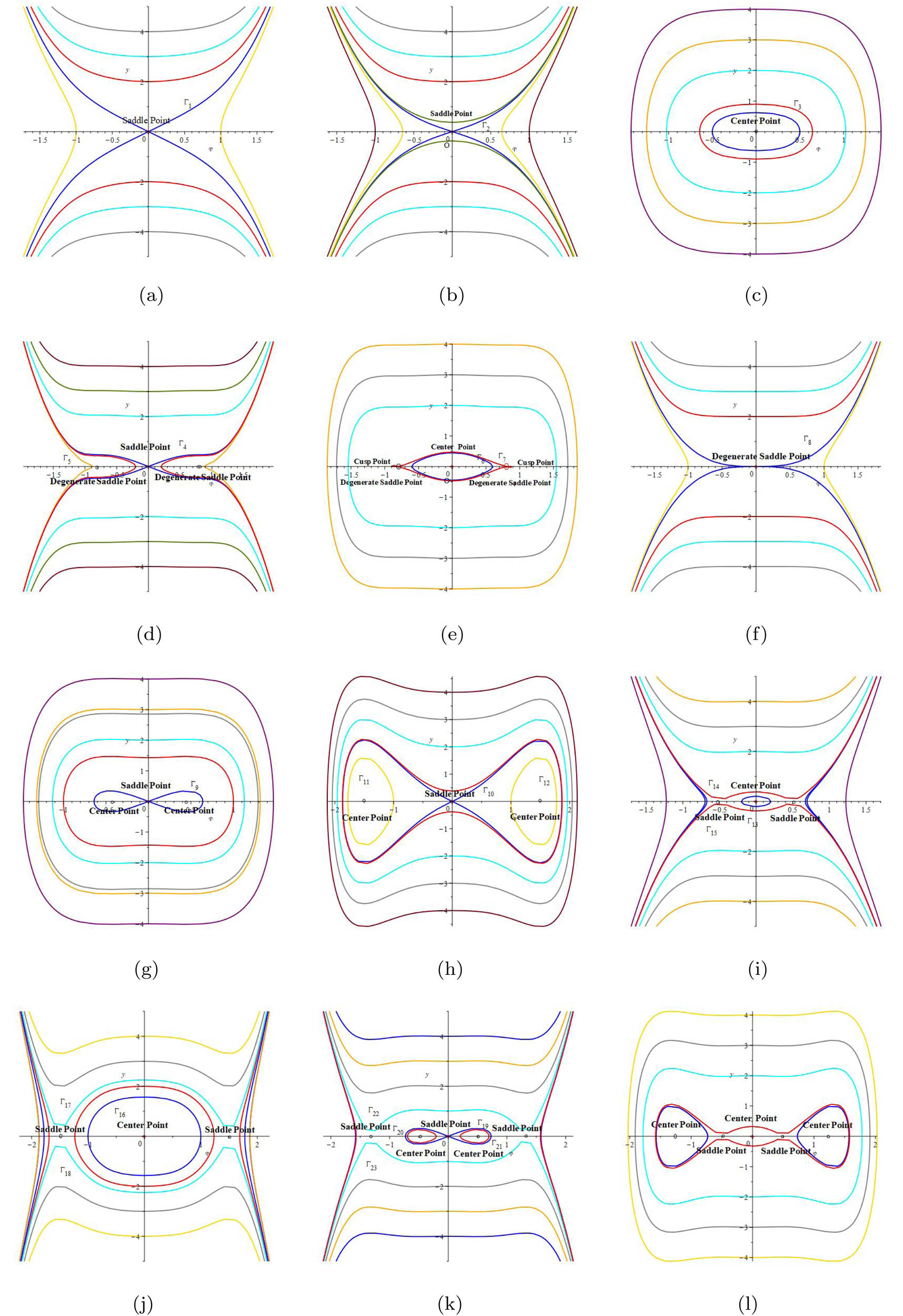
2D phase portraits of system (2.7): (a)
Case 2
In this situation, system (2.7) has three equilibrium points
Case 3
In this case, system (2.7) has three equilibrium points
Case 4
In the event, system (2.7) has the unique equilibrium point
Case 5
In this situation, system (2.7) has three equilibrium points
Case 6
In this case, system (2.7) has three equilibrium points
Case 7
In the event, system (2.7) has five equilibrium points
Case 8
In this situation, system (2.7) has five equilibrium points
2.3 Perturbation analysis of system (1.1)
In practical problems, there are many small changes that affect the system. It is very meaningful to study the impact of small changes in the system on overall properties. We express small changes as a perturbation term, and when the system is based on a fundamental assumption that it is subject to small disturbances, we analyze the impact of small disturbances on the system. At the same time, the changes in system properties can be approximated by making small modifications to the original state. Next, system (2.7) with perturbation term is represented as follows:
where
When
When
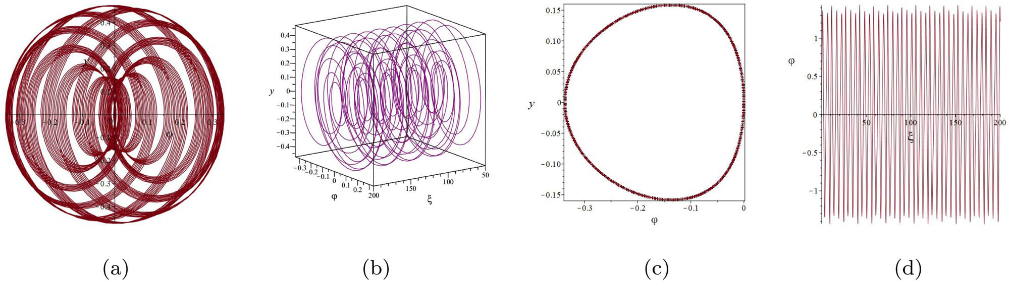
Due to the different effects of different types of perturbations on the system, and the varying effects of perturbations on the system when the system parameters and initial values are different, in order to understand these characteristics, numerical calculations and visualization are used to draw 2D and 3D phase portraits with different types of perturbation terms under different parameter conditions using Maple software. In addition, since continuous systems are difficult to observe motion trajectories and analyze laws in high-dimensional situations, discretization and dimensionality reduction are performed on high-dimensional continuous systems, transforming the continuous trajectories that are originally difficult to directly observe and analyze in phase space into discrete points on the cross-section, thus simplifying the complexity of the problem. Here, the Poincaré sections are drawn, and the distribution law on the cross-section can reflect the motion characteristics of the system. Of course, considering the impact of changes in system parameters, we can also discuss sensitivity analysis of parameters and draw sensitivity analysis figures.
When
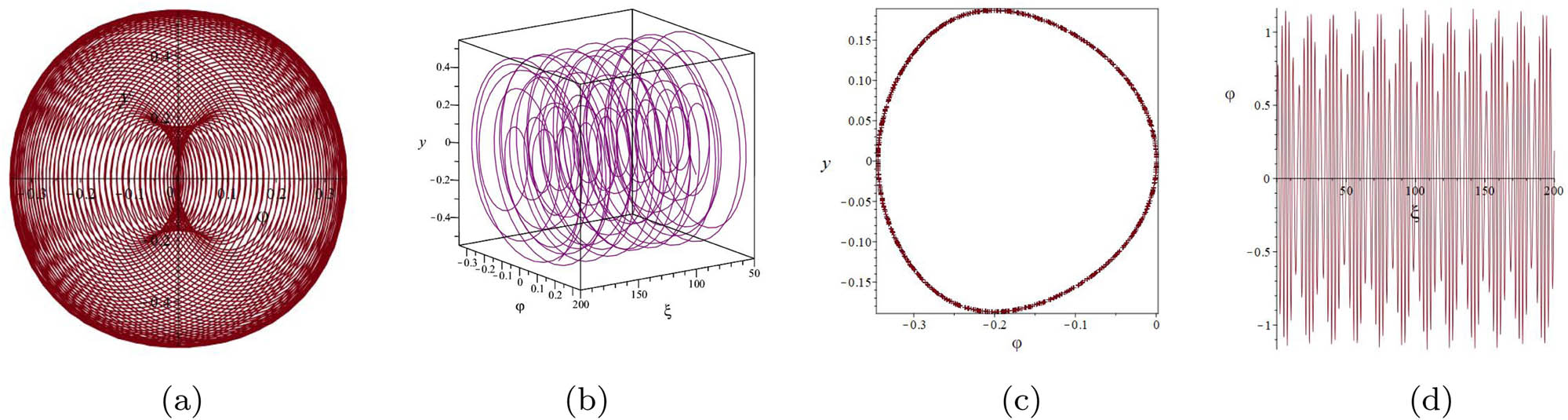
Perturbation analysis of system (2.10) with
Perturbation analysis of system (2.10) with

Perturbation analysis of system (2.10) with

Perturbation analysis of system (2.10) with

Perturbation analysis of system (2.10) with

Perturbation analysis of system (2.10) with

Perturbation analysis of system (2.10) with
When

Perturbation analysis of system (2.10) with

Perturbation analysis of system (2.10) with
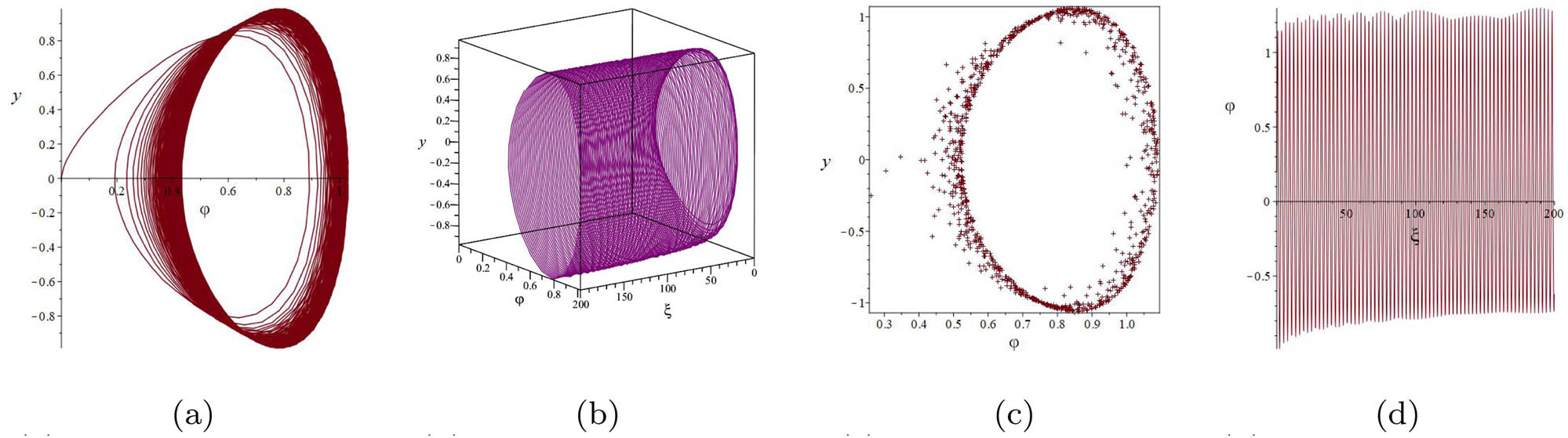
Perturbation analysis of system (2.10) with

Perturbation analysis of system (2.10) with

Perturbation analysis of system (2.10) with

Perturbation analysis of system (2.10) with
Through the visualization and numerical calculation, we can see that when system (2.10) is subjected to triangular periodic perturbation
3 Modulation instability analysis
Through qualitative analysis of the dynamic behavior of Eq. (1.1), we find that optical solitons may exhibit instability during fiber propagation due to the influence of perturbations on Eq. (1.1). This instability arises from the modulation effect on the steady-state caused by the interaction of nonlinear and dispersion effects.
Considering the combined effect of second-order dispersion and nonlinear effects, and taking into account the influence of perturbations, it is assumed that Eq. (1.1) has the following steady-state analytical solution
From Eq. (3.1), it can be seen that the expression of perturbation
where
Eq. (3.1) and Eq. (3.2) provide two homogeneous equations about
From the dispersion relationship of Eq. (3.3), we can obtain that the stability of steady-state solution under perturbations mainly depends on whether the transmitted beam in the fiber is in the normal dispersion region or the anomalous dispersion region.
When
We can obtain the gain of perturbation
In Figure 15, we can see that the gain spectrum

MI gain of
4 Conclusion
In this work, we mainly focus on the generalized coupled fractional nonlinear Helmholtz equation with cubic and quintic nonlinear effects in fiber optic propagation. In order to understand the dynamic behavior of the equation, through processes such as fractional derivatives, traveling wave transformations, and linear transformations, the equation is transformed into a two-dimensional planar dynamical system. Then through qualitative analysis, including phase portrait and bifurcation, parameter sensitivity analysis, the dynamic behavior of the system is comprehensively revealed. Meanwhile, considering that the stability of the system may be affected by disturbances, we analyze the dynamic behavior of the system under two different types of disturbances and provide possible reasons for the changes. Finally, the conditions for the system to maintain stability are provided through modulation instability. Due to the fact that the original equation is a fractional-order partial differential equation, the degree of its nonlinear terms is relatively high, reaching three and five degrees. Under the interaction between the nonlinear and dispersion terms, light waves produce self-modulation and self-steeping effects. When the interaction between the nonlinear and dispersion terms reaches equilibrium, optical solitons can be formed. Meanwhile, this interaction inevitably leads to modulation of the steady state, resulting in modulation instability. The study of modulation instability not only helps to deepen the understanding of the essence of nonlinear optical phenomena, but also provides new technological means and solutions for fields such as fiber optic communication and optical information processing. When we make a series of transformations to the system, we may overlook some of the effects, but such processing is a necessary means of analysis. In future research, different methods can be considered and comparative analysis can be conducted.
Acknowledgments
The authors thank Key Laboratory of Pattern Recognition and Intelligent Information Processing of Sichuan, Chengdu University, Chengdu, China (Grant No. MSSB-2024-07) and funding of V.C. & V.R. Key Lab of Sichuan Provence (Grant No. SCVCVR2024.08VS) for supporting this work.
-
Funding information: This work was supported by Key Laboratory of Pattern Recognition and Intelligent Information Processing of Sichuan (Grant No. MSSB-2024-07), Chengdu University, Chengdu, China. This study was supported by funding of V.C. and V.R. Key Lab of Sichuan Provence (Grant No. SCVCVR2024.08VS).
-
Author contributions: All authors have accepted responsibility for the entire content of this manuscript and approved its submission.
-
Conflict of interest: The authors state no conflict of interest.
-
Data availability statement: The datasets generated and/or analyzed during the current study are available from the corresponding author on reasonable request.
References
[1] Joshi MP, Bhosale S, Vyawahare VA. Comparative study of integer-order and fractional-order artificial neural networks: Application for mathematical function generation. e-Prime-Adv Electr Eng Electr Energy. 2024;8:100601. 10.1016/j.prime.2024.100601Search in Google Scholar
[2] Uddin M, Ullah Jan H, Usman M. RBF-PS method for approximation and eventual periodicity of fractional and integer type KdV equations. Partial Differ Equ Appl Math. 2022;5:100288. 10.1016/j.padiff.2022.100288Search in Google Scholar
[3] Yan S, Jiang D, Cui Y, Zhang H, Li L, Jiang J. A fractional-order hyperchaotic system that is period in integer-order case and its application in a novel high-quality color image encryption algorithm. Chaos Solitons Fractals. 2024;182:114793. 10.1016/j.chaos.2024.114793Search in Google Scholar
[4] Arimi HJ, Eslami M, Ansari A. Numerical study of distributed-order Bessel fractional derivative with application to Euler-Poisson-Darboux equation. Commun Nonl Sci Numer Simulat. 2024;133:107950. 10.1016/j.cnsns.2024.107950Search in Google Scholar
[5] Ruggieri M, Speciale MP. Asymptotic expansion method with respect to a small parameter for fractional differential equations with Riemann–Liouville derivate. Commun Nonl Sci Numer Simulat. 2024;138:108234. 10.1016/j.cnsns.2024.108234Search in Google Scholar
[6] Swati S, Nilam. Fractional order model using Caputo fractional derivative to analyse the effects of social media on mental health during Covid-19. Alexandr Eng J. 2024;92:336–45. 10.1016/j.aej.2024.02.049Search in Google Scholar
[7] MacDonald CL, Bhattacharya N, Sprouse BP, Silva GA. Efficient computation of the Grünwald–Letnikov fractional diffusion derivative using adaptive time step memory. J Comput Phys. 2015;297:221–36. 10.1016/j.jcp.2015.04.048Search in Google Scholar
[8] Fareed AF, Semary MS, Hassan HN. An approximate solution of fractional-order Riccati equations based on controlled Picardas method with Atangana’s fractional derivative. Alexandr Eng J. 2022;61:3673–8. 10.1016/j.aej.2021.09.009Search in Google Scholar
[9] Liu Y, Yang J, Liu Z, Xu Q. Meshfree methods for the time fractional Navier–Stokes equations. Eng Anal Boundary Elements. 2024;166:105823. 10.1016/j.enganabound.2024.105823Search in Google Scholar
[10] Hao J, Li M. A new class of fractional Navier–Stokes system coupled with multivalued boundary conditions. Commun Nonl Sci Numer Simulat. 2024;136:108098. 10.1016/j.cnsns.2024.108098Search in Google Scholar
[11] Chen J, Li X, Shao Y. Numerical analysis of fractional-order Black–Scholes option pricing model with band equation method. J Comput Appl Math. 2024;451:115998. 10.1016/j.cam.2024.115998Search in Google Scholar
[12] Zhao T, Zhao L. Jacobian spectral collocation method for spatio-temporal coupled Fokker–Planck equation with variable-order fractional derivative. Commun Nonl Sci Numer Simulat. 2023;124:107305. 10.1016/j.cnsns.2023.107305Search in Google Scholar
[13] Faridi WA, A-M Wazwaz, Mostafa AM, Myrzakulov R, Umurzakhova Z. The Lie point symmetry criteria and formation of exact analytical solutions for Kairat-II equation: Paul-Painlevé approach. Chaos Solitons Fractals. 2024;182:114745. 10.1016/j.chaos.2024.114745Search in Google Scholar
[14] Azar EA, Jalili B, Azar AA, Jalili P, Atazadeh M, Ganji DD An exact analytical solution of the Emden-Chandrasekhar equation for self-gravitating isothermal gas spheres in the theory of stellar structures. Phys Dark Univ. 2023;42:101309. 10.1016/j.dark.2023.101309Search in Google Scholar
[15] Mahor TC, Mishra R, Jain R. Analytical solutions of linear fractional partial differential equations using fractional Fourier transform. J Comput Appl Math. 2021;385:113202. 10.1016/j.cam.2020.113202Search in Google Scholar
[16] Abd Elbary FE, Ali KK, Semary MS. A new approach for solving fractional Kundu-Eckhaus equation and fractional massive Thirring model using controlled Picardas technique with ρ-Laplace transform. Partial Differ Equ Appl Math. 2024;10:100675. 10.1016/j.padiff.2024.100675Search in Google Scholar
[17] Khabiri A, Asgari A, Taghipour R. Analysis of fractional Euler-Bernoulli bending beams using Greenas function method. Alexandr Eng J. 2024;1060:312–27. 10.1016/j.aej.2024.07.023Search in Google Scholar
[18] Mohamed MZ, Elzaki TM. Applications of new integral transform for linear and nonlinear fractional partial differential equations. J King Saud Univ-Sci. 2020;32:544–9. 10.1016/j.jksus.2018.08.003Search in Google Scholar
[19] Ghanim F, Khan FS, Al-Janaby HF, Ali AH. A new hybrid special function class and numerical technique for multi-order fractional differential equations. Alexandr Eng J. 2024;104:603–13. 10.1016/j.aej.2024.08.009Search in Google Scholar
[20] Agrawal K, Kumar S, Alkahtani BS, Alzaid SS. A numerical study on fractional-order financial system with chaotic and Lyapunov stability analysis. Results Phys. 2024;60:107685. 10.1016/j.rinp.2024.107685Search in Google Scholar
[21] Wang H, Wang J, Zhang S, Zhang Y. A time splitting Chebyshev-Fourier spectral method for the time-dependent rotating nonlocal Schrödinger equation in polar coordinates. J Computat Phys. 2024;498:112680. 10.1016/j.jcp.2023.112680Search in Google Scholar
[22] Carbonaro A, Dragicević O. On semigroup maximal operators associated with divergence-form operators with complex coefficients. J Differ Equ. 2024;394:98–119. 10.1016/j.jde.2024.02.032Search in Google Scholar
[23] Qing L, Li X. Meshless analysis of fractional diffusion-wave equations by generalized finite difference method. Appl Math Lett. 2024;157:109204. 10.1016/j.aml.2024.109204Search in Google Scholar
[24] Akrami MH, Poya A, Zirak MA. Solving the general form of the fractional Black–Scholes with two assets through reconstruction variational iteration method. Results Appl Math. 2024;22:100444. 10.1016/j.rinam.2024.100444Search in Google Scholar
[25] Huang Y, Rad NT, Skandari MH, Tohidi E. A spectral collocation scheme for solving nonlinear delay distributed-order fractional equations. J Comput Appl Math. 2024;456:116227. 10.1016/j.cam.2024.116227Search in Google Scholar
[26] Li Z, Zhao S. Bifurcation, chaotic behavior and solitary wave solutions for the Akbota equation. AIMS Math. 2024;9:22590–601. 10.3934/math.20241100Search in Google Scholar
[27] Fukui T, Li Q Pei D. Bifurcation model for nonlinear equations. Hokkaido Math J. 2024;53(2):349–75. 10.14492/hokmj/2022-674Search in Google Scholar
[28] Zhang K, Li Z. Bifurcation, chaotic pattern and optical soliton solutions of generalized nonlinear Schrödinger equation. Results Phys. 2023;51:106721. 10.1016/j.rinp.2023.106721Search in Google Scholar
[29] Nasreen N, Muhammad J, Jhangeer A. Dynamics of fractional optical solitary waves to the cubic–quintic coupled nonlinear Helmholtz equation. Partial Differ Equ Appl Math. 2024;11:100812. 10.1016/j.padiff.2024.100812Search in Google Scholar
[30] Alsaud H, Youssoufa M, Inc M, Inan IE, Bicer H. Some optical solitons and modulation instability analysis of (3+1)-dimensional nonlinear Schrödinger and coupled nonlinear Helmholtz equations. Opt Quantum Electron. 2024;56:1138. 10.1007/s11082-024-06851-4Search in Google Scholar
[31] Atangana A, Baleanu D, Alsaedi A. Analysis of time-fractional Hunter-Saxton equation: a model of neumatic liquid crystal. Open Phys. 2016;14:145–9. 10.1515/phys-2016-0010Search in Google Scholar
[32] Chen T, Huang L, Yu P. Center condition and bifurcation of limit cycles for quadratic switching systems with a nilpotent equilibrium point. J Differ Equ. 2021;303:326–68. 10.1016/j.jde.2021.09.030Search in Google Scholar
© 2025 the author(s), published by De Gruyter
This work is licensed under the Creative Commons Attribution 4.0 International License.
Articles in the same Issue
- Research Articles
- Single-step fabrication of Ag2S/poly-2-mercaptoaniline nanoribbon photocathodes for green hydrogen generation from artificial and natural red-sea water
- Abundant new interaction solutions and nonlinear dynamics for the (3+1)-dimensional Hirota–Satsuma–Ito-like equation
- A novel gold and SiO2 material based planar 5-element high HPBW end-fire antenna array for 300 GHz applications
- Explicit exact solutions and bifurcation analysis for the mZK equation with truncated M-fractional derivatives utilizing two reliable methods
- Optical and laser damage resistance: Role of periodic cylindrical surfaces
- Numerical study of flow and heat transfer in the air-side metal foam partially filled channels of panel-type radiator under forced convection
- Water-based hybrid nanofluid flow containing CNT nanoparticles over an extending surface with velocity slips, thermal convective, and zero-mass flux conditions
- Dynamical wave structures for some diffusion--reaction equations with quadratic and quartic nonlinearities
- Solving an isotropic grey matter tumour model via a heat transfer equation
- Study on the penetration protection of a fiber-reinforced composite structure with CNTs/GFP clip STF/3DKevlar
- Influence of Hall current and acoustic pressure on nanostructured DPL thermoelastic plates under ramp heating in a double-temperature model
- Applications of the Belousov–Zhabotinsky reaction–diffusion system: Analytical and numerical approaches
- AC electroosmotic flow of Maxwell fluid in a pH-regulated parallel-plate silica nanochannel
- Interpreting optical effects with relativistic transformations adopting one-way synchronization to conserve simultaneity and space–time continuity
- Modeling and analysis of quantum communication channel in airborne platforms with boundary layer effects
- Theoretical and numerical investigation of a memristor system with a piecewise memductance under fractal–fractional derivatives
- Tuning the structure and electro-optical properties of α-Cr2O3 films by heat treatment/La doping for optoelectronic applications
- High-speed multi-spectral explosion temperature measurement using golden-section accelerated Pearson correlation algorithm
- Dynamic behavior and modulation instability of the generalized coupled fractional nonlinear Helmholtz equation with cubic–quintic term
- Study on the duration of laser-induced air plasma flash near thin film surface
- Exploring the dynamics of fractional-order nonlinear dispersive wave system through homotopy technique
- The mechanism of carbon monoxide fluorescence inside a femtosecond laser-induced plasma
- Numerical solution of a nonconstant coefficient advection diffusion equation in an irregular domain and analyses of numerical dispersion and dissipation
- Numerical examination of the chemically reactive MHD flow of hybrid nanofluids over a two-dimensional stretching surface with the Cattaneo–Christov model and slip conditions
- Impacts of sinusoidal heat flux and embraced heated rectangular cavity on natural convection within a square enclosure partially filled with porous medium and Casson-hybrid nanofluid
- Stability analysis of unsteady ternary nanofluid flow past a stretching/shrinking wedge
- Solitonic wave solutions of a Hamiltonian nonlinear atom chain model through the Hirota bilinear transformation method
- Bilinear form and soltion solutions for (3+1)-dimensional negative-order KdV-CBS equation
- Solitary chirp pulses and soliton control for variable coefficients cubic–quintic nonlinear Schrödinger equation in nonuniform management system
- Influence of decaying heat source and temperature-dependent thermal conductivity on photo-hydro-elasto semiconductor media
- Dissipative disorder optimization in the radiative thin film flow of partially ionized non-Newtonian hybrid nanofluid with second-order slip condition
- Bifurcation, chaotic behavior, and traveling wave solutions for the fractional (4+1)-dimensional Davey–Stewartson–Kadomtsev–Petviashvili model
- New investigation on soliton solutions of two nonlinear PDEs in mathematical physics with a dynamical property: Bifurcation analysis
- Mathematical analysis of nanoparticle type and volume fraction on heat transfer efficiency of nanofluids
- Creation of single-wing Lorenz-like attractors via a ten-ninths-degree term
- Optical soliton solutions, bifurcation analysis, chaotic behaviors of nonlinear Schrödinger equation and modulation instability in optical fiber
- Chaotic dynamics and some solutions for the (n + 1)-dimensional modified Zakharov–Kuznetsov equation in plasma physics
- Fractal formation and chaotic soliton phenomena in nonlinear conformable Heisenberg ferromagnetic spin chain equation
- Single-step fabrication of Mn(iv) oxide-Mn(ii) sulfide/poly-2-mercaptoaniline porous network nanocomposite for pseudo-supercapacitors and charge storage
- Novel constructed dynamical analytical solutions and conserved quantities of the new (2+1)-dimensional KdV model describing acoustic wave propagation
- Tavis–Cummings model in the presence of a deformed field and time-dependent coupling
- Spinning dynamics of stress-dependent viscosity of generalized Cross-nonlinear materials affected by gravitationally swirling disk
- Design and prediction of high optical density photovoltaic polymers using machine learning-DFT studies
- Robust control and preservation of quantum steering, nonlocality, and coherence in open atomic systems
- Coating thickness and process efficiency of reverse roll coating using a magnetized hybrid nanomaterial flow
- Dynamic analysis, circuit realization, and its synchronization of a new chaotic hyperjerk system
- Decoherence of steerability and coherence dynamics induced by nonlinear qubit–cavity interactions
- Finite element analysis of turbulent thermal enhancement in grooved channels with flat- and plus-shaped fins
- Modulational instability and associated ion-acoustic modulated envelope solitons in a quantum plasma having ion beams
- Statistical inference of constant-stress partially accelerated life tests under type II generalized hybrid censored data from Burr III distribution
- On solutions of the Dirac equation for 1D hydrogenic atoms or ions
- Entropy optimization for chemically reactive magnetized unsteady thin film hybrid nanofluid flow on inclined surface subject to nonlinear mixed convection and variable temperature
- Stability analysis, circuit simulation, and color image encryption of a novel four-dimensional hyperchaotic model with hidden and self-excited attractors
- A high-accuracy exponential time integration scheme for the Darcy–Forchheimer Williamson fluid flow with temperature-dependent conductivity
- Novel analysis of fractional regularized long-wave equation in plasma dynamics
- Development of a photoelectrode based on a bismuth(iii) oxyiodide/intercalated iodide-poly(1H-pyrrole) rough spherical nanocomposite for green hydrogen generation
- Investigation of solar radiation effects on the energy performance of the (Al2O3–CuO–Cu)/H2O ternary nanofluidic system through a convectively heated cylinder
- Quantum resources for a system of two atoms interacting with a deformed field in the presence of intensity-dependent coupling
- Studying bifurcations and chaotic dynamics in the generalized hyperelastic-rod wave equation through Hamiltonian mechanics
- A new numerical technique for the solution of time-fractional nonlinear Klein–Gordon equation involving Atangana–Baleanu derivative using cubic B-spline functions
- Interaction solutions of high-order breathers and lumps for a (3+1)-dimensional conformable fractional potential-YTSF-like model
- Hydraulic fracturing radioactive source tracing technology based on hydraulic fracturing tracing mechanics model
- Numerical solution and stability analysis of non-Newtonian hybrid nanofluid flow subject to exponential heat source/sink over a Riga sheet
- Numerical investigation of mixed convection and viscous dissipation in couple stress nanofluid flow: A merged Adomian decomposition method and Mohand transform
- Effectual quintic B-spline functions for solving the time fractional coupled Boussinesq–Burgers equation arising in shallow water waves
- Analysis of MHD hybrid nanofluid flow over cone and wedge with exponential and thermal heat source and activation energy
- Solitons and travelling waves structure for M-fractional Kairat-II equation using three explicit methods
- Impact of nanoparticle shapes on the heat transfer properties of Cu and CuO nanofluids flowing over a stretching surface with slip effects: A computational study
- Computational simulation of heat transfer and nanofluid flow for two-sided lid-driven square cavity under the influence of magnetic field
- Irreversibility analysis of a bioconvective two-phase nanofluid in a Maxwell (non-Newtonian) flow induced by a rotating disk with thermal radiation
- Hydrodynamic and sensitivity analysis of a polymeric calendering process for non-Newtonian fluids with temperature-dependent viscosity
- Exploring the peakon solitons molecules and solitary wave structure to the nonlinear damped Kortewege–de Vries equation through efficient technique
- Modeling and heat transfer analysis of magnetized hybrid micropolar blood-based nanofluid flow in Darcy–Forchheimer porous stenosis narrow arteries
- Activation energy and cross-diffusion effects on 3D rotating nanofluid flow in a Darcy–Forchheimer porous medium with radiation and convective heating
- Insights into chemical reactions occurring in generalized nanomaterials due to spinning surface with melting constraints
- Influence of a magnetic field on double-porosity photo-thermoelastic materials under Lord–Shulman theory
- Soliton-like solutions for a nonlinear doubly dispersive equation in an elastic Murnaghan's rod via Hirota's bilinear method
- Analytical and numerical investigation of exact wave patterns and chaotic dynamics in the extended improved Boussinesq equation
- Nonclassical correlation dynamics of Heisenberg XYZ states with (x, y)-spin--orbit interaction, x-magnetic field, and intrinsic decoherence effects
- Exact traveling wave and soliton solutions for chemotaxis model and (3+1)-dimensional Boiti–Leon–Manna–Pempinelli equation
- Unveiling the transformative role of samarium in ZnO: Exploring structural and optical modifications for advanced functional applications
- On the derivation of solitary wave solutions for the time-fractional Rosenau equation through two analytical techniques
- Analyzing the role of length and radius of MWCNTs in a nanofluid flow influenced by variable thermal conductivity and viscosity considering Marangoni convection
- Advanced mathematical analysis of heat and mass transfer in oscillatory micropolar bio-nanofluid flows via peristaltic waves and electroosmotic effects
- Exact bound state solutions of the radial Schrödinger equation for the Coulomb potential by conformable Nikiforov–Uvarov approach
- Some anisotropic and perfect fluid plane symmetric solutions of Einstein's field equations using killing symmetries
- Nonlinear dynamics of the dissipative ion-acoustic solitary waves in anisotropic rotating magnetoplasmas
- Curves in multiplicative equiaffine plane
- Exact solution of the three-dimensional (3D) Z2 lattice gauge theory
- Propagation properties of Airyprime pulses in relaxing nonlinear media
- Symbolic computation: Analytical solutions and dynamics of a shallow water wave equation in coastal engineering
- Wave propagation in nonlocal piezo-photo-hygrothermoelastic semiconductors subjected to heat and moisture flux
- Comparative reaction dynamics in rotating nanofluid systems: Quartic and cubic kinetics under MHD influence
- Laplace transform technique and probabilistic analysis-based hypothesis testing in medical and engineering applications
- Physical properties of ternary chloro-perovskites KTCl3 (T = Ge, Al) for optoelectronic applications
- Gravitational length stretching: Curvature-induced modulation of quantum probability densities
- The search for the cosmological cold dark matter axion – A new refined narrow mass window and detection scheme
- A comparative study of quantum resources in bipartite Lipkin–Meshkov–Glick model under DM interaction and Zeeman splitting
- PbO-doped K2O–BaO–Al2O3–B2O3–TeO2-glasses: Mechanical and shielding efficacy
- Nanospherical arsenic(iii) oxoiodide/iodide-intercalated poly(N-methylpyrrole) composite synthesis for broad-spectrum optical detection
- Sine power Burr X distribution with estimation and applications in physics and other fields
- Numerical modeling of enhanced reactive oxygen plasma in pulsed laser deposition of metal oxide thin films
- Dynamical analyses and dispersive soliton solutions to the nonlinear fractional model in stratified fluids
- Computation of exact analytical soliton solutions and their dynamics in advanced optical system
- An innovative approximation concerning the diffusion and electrical conductivity tensor at critical altitudes within the F-region of ionospheric plasma at low latitudes
- An analytical investigation to the (3+1)-dimensional Yu–Toda–Sassa–Fukuyama equation with dynamical analysis: Bifurcation
- Swirling-annular-flow-induced instability of a micro shell considering Knudsen number and viscosity effects
- Numerical analysis of non-similar convection flows of a two-phase nanofluid past a semi-infinite vertical plate with thermal radiation
- MgO NPs reinforced PCL/PVC nanocomposite films with enhanced UV shielding and thermal stability for packaging applications
- Optimal conditions for indoor air purification using non-thermal Corona discharge electrostatic precipitator
- Investigation of thermal conductivity and Raman spectra for HfAlB, TaAlB, and WAlB based on first-principles calculations
- Tunable double plasmon-induced transparency based on monolayer patterned graphene metamaterial
- DSC: depth data quality optimization framework for RGBD camouflaged object detection
- A new family of Poisson-exponential distributions with applications to cancer data and glass fiber reliability
- Numerical investigation of couple stress under slip conditions via modified Adomian decomposition method
- Monitoring plateau lake area changes in Yunnan province, southwestern China using medium-resolution remote sensing imagery: applicability of water indices and environmental dependencies
- Heterodyne interferometric fiber-optic gyroscope
- Exact solutions of Einstein’s field equations via homothetic symmetries of non-static plane symmetric spacetime
- A widespread study of discrete entropic model and its distribution along with fluctuations of energy
- Empirical model integration for accurate charge carrier mobility simulation in silicon MOSFETs
- The influence of scattering correction effect based on optical path distribution on CO2 retrieval
- Anisotropic dissociation and spectral response of 1-Bromo-4-chlorobenzene under static directional electric fields
- Role of tungsten oxide (WO3) on thermal and optical properties of smart polymer composites
- Analysis of iterative deblurring: no explicit noise
- The influence of anisotropy of InP on its elasticity and phonon properties
- Review Article
- Examination of the gamma radiation shielding properties of different clay and sand materials in the Adrar region
- Erratum
- Erratum to “On Soliton structures in optical fiber communications with Kundu–Mukherjee–Naskar model (Open Physics 2021;19:679–682)”
- Special Issue on Fundamental Physics from Atoms to Cosmos - Part II
- Possible explanation for the neutron lifetime puzzle
- Special Issue on Nanomaterial utilization and structural optimization - Part III
- Numerical investigation on fluid-thermal-electric performance of a thermoelectric-integrated helically coiled tube heat exchanger for coal mine air cooling
- Special Issue on Nonlinear Dynamics and Chaos in Physical Systems
- Analysis of the fractional relativistic isothermal gas sphere with application to neutron stars
- Abundant wave symmetries in the (3+1)-dimensional Chafee–Infante equation through the Hirota bilinear transformation technique
- Successive midpoint method for fractional differential equations with nonlocal kernels: Error analysis, stability, and applications
- Novel exact solitons to the fractional modified mixed-Korteweg--de Vries model with a stability analysis