Stability analysis, circuit simulation, and color image encryption of a novel four-dimensional hyperchaotic model with hidden and self-excited attractors
-
Tarek M. Abed-Elhameed
 and
Mansour E. Ahmed
and
Mansour E. Ahmed

Abstract
A new four-dimensional hyperchaotic model (4-DHM) with eight parameters is examined in this work. Depending on how two of these parameters are chosen, this model may contain equilibrium points or not. Therefore, we may choose a value that will make the corresponding attractor either hidden or self-excited. In this model, we consider the two scenarios and analyze the dynamics of the two instances. The numerical simulation of the novel 4-DHM is shown together with bifurcation diagrams, the Lyapunov exponent, and an examination of equilibrium and stability. The novel 4-DHM may be used in many science and engineering applications, such as electronic circuits and image encryption. A physical implementation is added to the electronic circuit’s MATLAB Simulink to confirm that the new 4-DHM can be built. The results of the numerical analysis and electronic circuit simulation of our model were in a good agreement. The color image’s encryption, decryption, histogram analysis, information entropy, correlation coefficient, number of pixels change rate, and unified average changing intensity are examined using the proposed model.
List of Abbreviations
- BDs
-
bifurcation diagrams
- 4-DHM
-
four-dimensional hyperchaotic model
- LEs
-
lyapunov exponents
- NPCR
-
number of pixel change rate
- RGB
-
red, green, blue (color model)
- UACI
-
unified average changing intensity
1 Introduction
Since Lorenz [1] discovered the first 3D autonomous chaotic system, chaos has adapted and grown significantly. Chaotic systems are important to dynamical systems due to their fascinating and complex dynamical properties. Some sciences, including biology, medicine, geology, image encoding, secure communication, and physics, may benefit from the study of chaotic systems [2–10]. Classical chaotic systems have already been identified in a number of instances over the past few decades [11–14]. Recently, many scientists have shown an increasing interest in studying chaotic and hyperchaotic dynamical systems [15–20]. For applications based on chaotic systems, hyperchaotic systems contribute to a crucial component [21–27].
Shilnikov’s criteria [28] state that there is a connection between chaotic attractors and the model equilibrium. In dissipative dynamical models, the presence of at least one unstable equilibrium point is a prerequisite for chaos. However, in order to confirm chaos in light of the finding of hidden attractors, the traditional Shilnikov criteria must be used. Attractors can be divided into two categories from a computational perspective: self-excited attractors and hidden attractors [29]. If any tiny neighborhoods of a stationary state are intersected by the basin of attraction of an attractor, it is referred to as a “self-excited attractor.” If not, it is called a hidden attraction. Hidden attractors are crucial in engineering applications because they enable unexpected and sometimes dangerous responses to perturbations in a structure, such as a bridge or an airplane wing [29–32].
Since the creation of Chua’s circuit [33], the study of chaotic circuits has attracted a lot of interest. Numerous chaotic (hyperchaotic)-producing nonlinear electronic circuits have been developed. A chaotic circuit is essentially a kind of chaotic system, and scholars usually use the electronic circuits to yield chaotic signals and demonstrate the physical existence of chaotic systems [34]. Some well-known examples of chaotic circuits are Chua’s circuit and the Lorenz system [35]. A hyperchaotic circuit is a chaotic circuit that has more than one positive Lyapunov exponent (LE), which means that it has more than one direction of instability and higher complexity [35]. Hyperchaos can be generated by adding some feedback controllers or nonlinear elements to the original chaotic circuits [35,36]. On the other hand, image encryption utilizing chaotic (or hyperchaotic) systems has garnered significant attention from researchers in recent years [37–39]. Masood et al. [37] introduced a novel approach for color image encryption based on DNA computing. Biban et al. explored image encryption employing an 8D hyperchaotic system combined with the Fibonacci Q-matrix [38]. Yan et al. introduced an innovative color image encryption technique utilizing a new three-dimensional chaotic mapping and DNA coding. As a result, applying chaotic (hyperchaotic) models to engineering practice through circuit implementation and image encryption has grown to be a crucial way for transferring chaotic (hyperchaotic) models from theory to practice. The circuit application and image encryption of chaotic (hyperchaotic) models have made significant progress up to this point.
Hu et al. [40] presented and studied a memristor-based VB2 chaotic model as
where
In this work, a new continuous-time, four-dimensional autonomous system is constructed, and its proposed scheme is obtained through the use of model (1.1). A new four-dimensional hyperchaotic model (4-DHM) based on model (1.1) is defined by
where
Our goal in this work is to introduce and investigate a new 4-DHM with self-excited and hidden attractors. The dynamics of the new 4-DHM with equilibrium or no equilibrium points are analyzed. Then, the LE, bifurcation diagram (BD), and phase portrait are used to examine the proposed hyperchaotic model. An electronic circuit for the new 4-DHM is being designed. The encryption, decryption, histogram analysis, information entropy, correlation coefficient, number of pixel change rate (NPCR), and Unified average changing intensity (UACI) of a color image are investigated based on the 4-DHM (1.2).
The rest of this work is arranged as follows: Section 2 provides a thorough examination of some basic dynamical properties of the 4-DHM (1.2). The 4-DHM (1.2) electronic circuit is found in Section 3. Comparing numerical and simulation findings, a good degree of agreement is obtained. Section 4 provides an analysis of encryption, decryption, histograms, information entropy, correlation coefficients, NPCR, and UACI for a color image using the 4-DHM (1.2). The conclusion of this research study is located in Section 5.
2 Basic dynamical properties of model (1.2)
In this section, we will study and discuss a few basic properties of the new 4-DHM model (1.2). Model (1.2) has eight parameters and nine terms, three of which are nonlinear. This model may or may not have equilibrium points, depending on how the parameters h and f are selected.
2.1 Equilibrium points
The equilibrium points of model (1.2) occur when
Clearly, one may derive
Remark 2.1
It is observed that one can attain hidden attractors or self-excited attractors for our model (1.2) by selecting suitable values for the model’s parameters
2.2 Symmetry and dissipation
The new 4-DHM model (1.2) does not have symmetry since it changes independently of the coordinate transformation. Model (1.2) is dissipative under the condition
When
2.3 Jacobian matrix and stability of equilibrium points
It is possible to determine the linear stability of the equilibrium points by computing the Jacobian matrix
The characteristic equation of (2.3) can be written as:
It is evident from the Routh–Hurwitz stability criterion that
2.4 Dynamics of model (1.2) with no equilibrium points
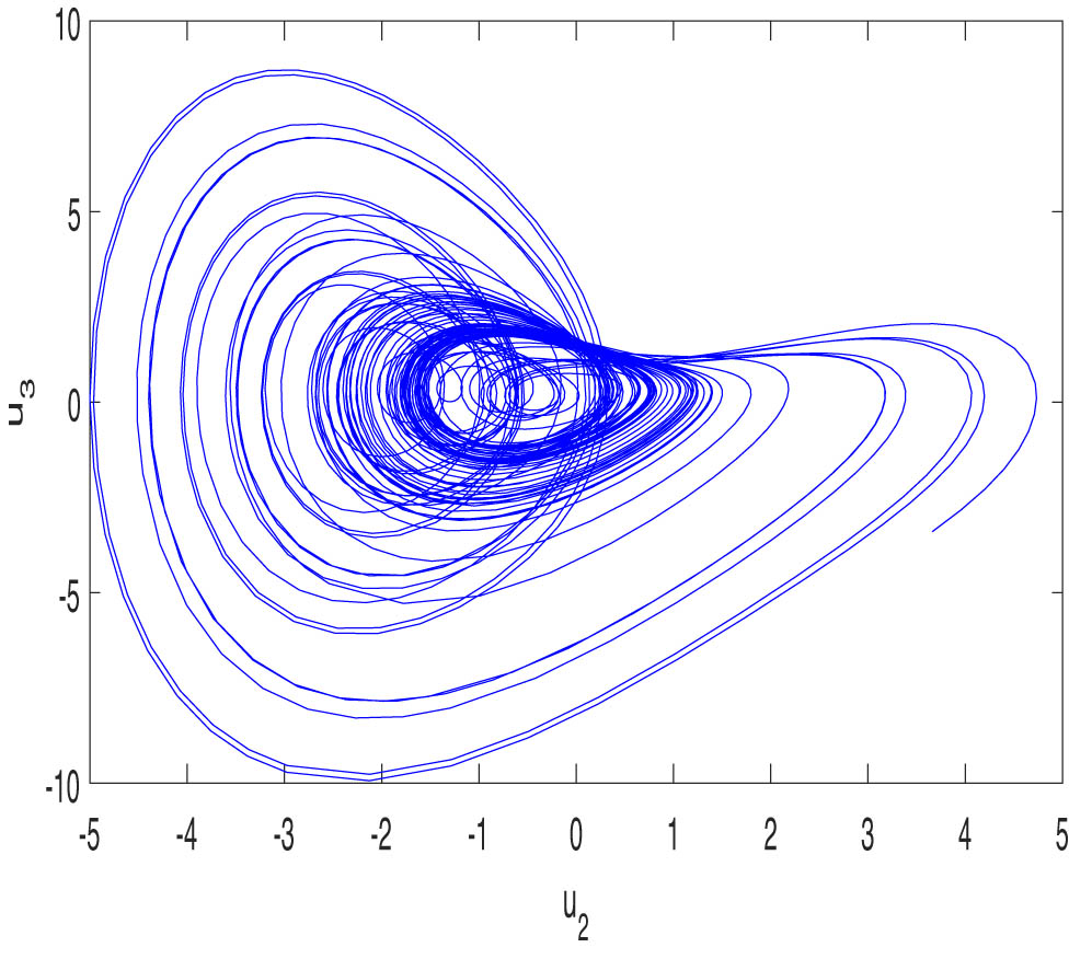
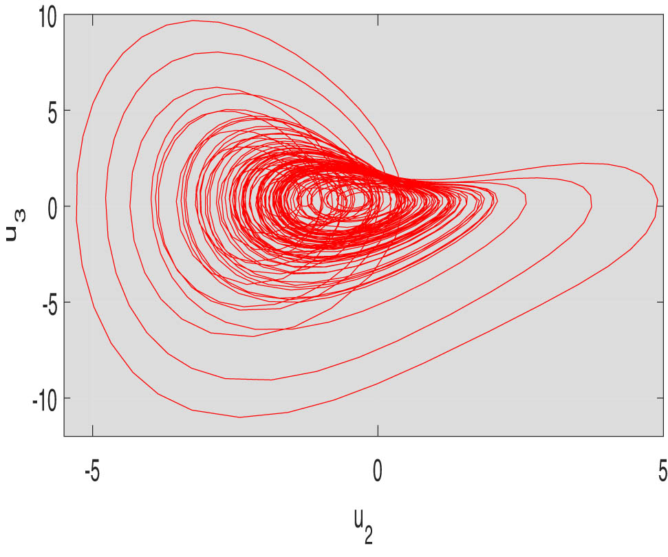
For the choice

Hyperchaotic hidden attractor of model (1.2) in the
Fix
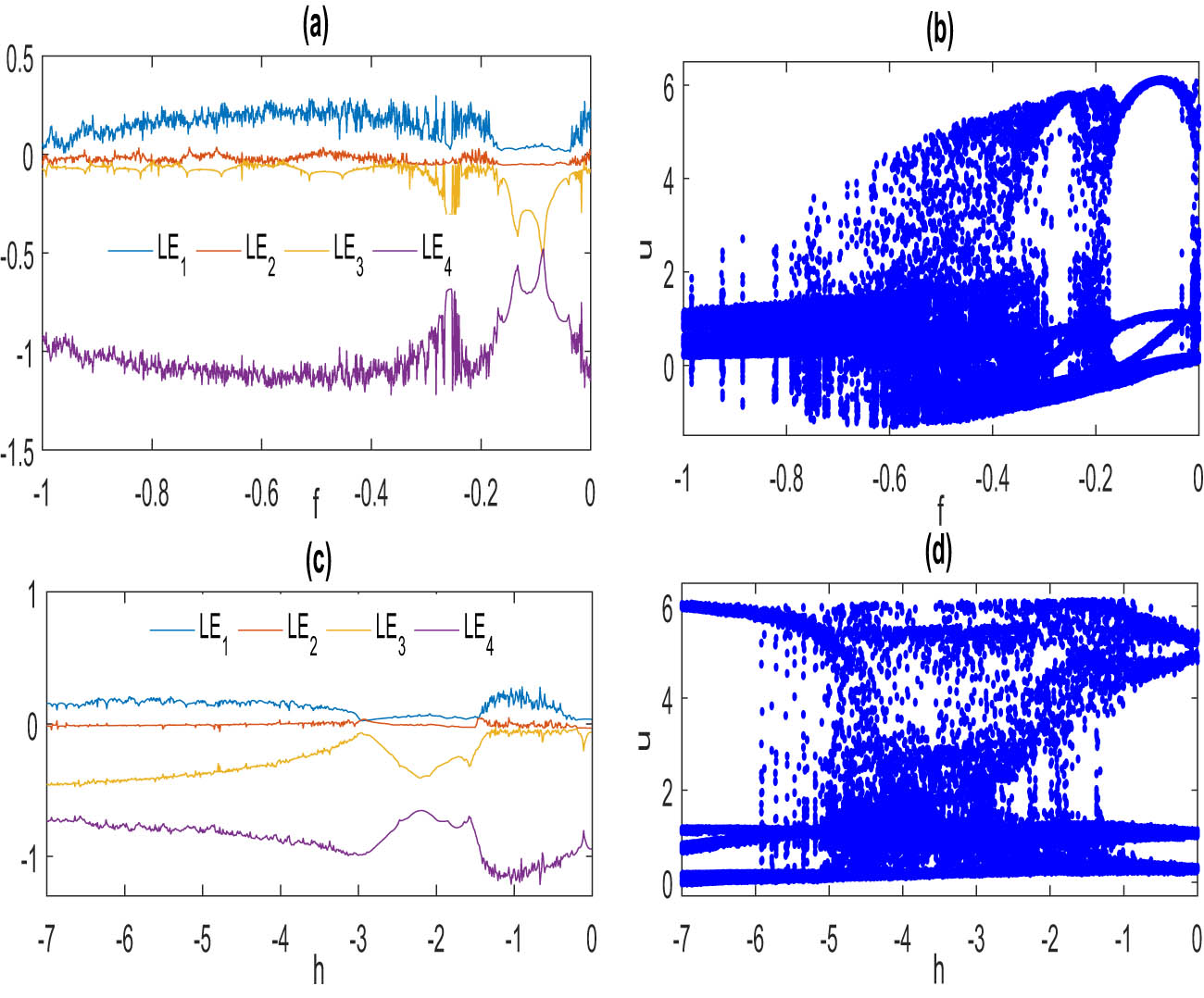
By calculating the LEs of model (1.2), it is clear that this model has chaotic and hyperchaotic solutions, as shown in Figure 2(a). The BD for the proposed hyperchaotic model is also provided in Figure 2(b) to indicate the path of chaos.
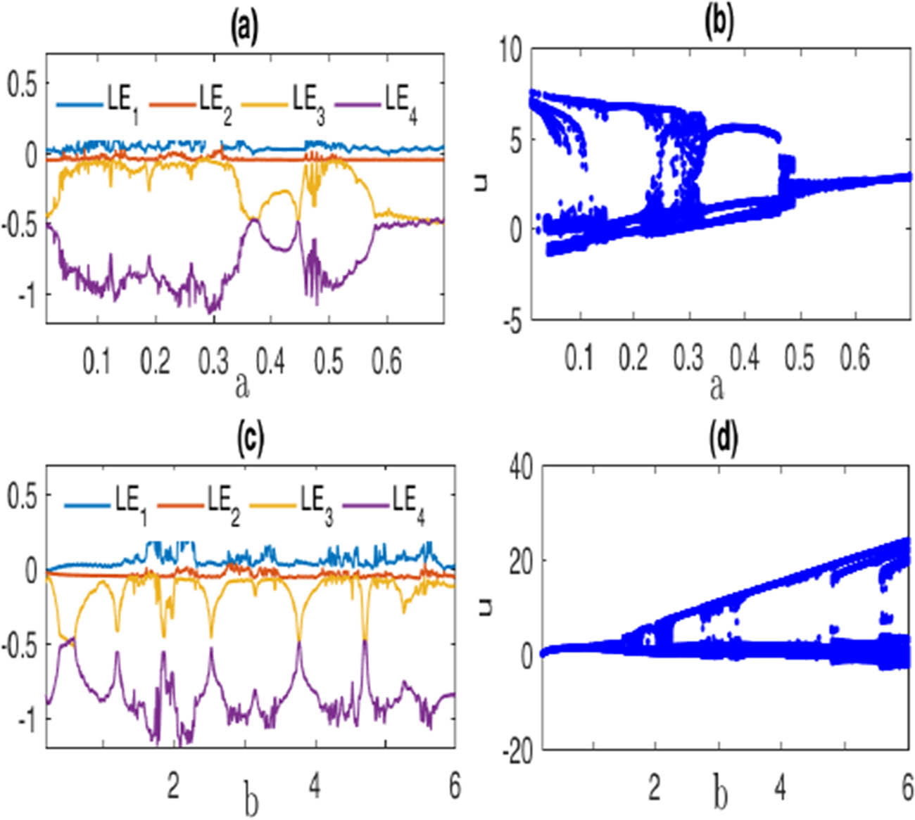
Dynamics of model (1.2) with the same initial values as Figure 1: (a) The corresponding LE for the parameter values
Fix
By the same way, Figures 3, 4, 5 show the LEs and BDs for the reminder parameters of model (1.2).
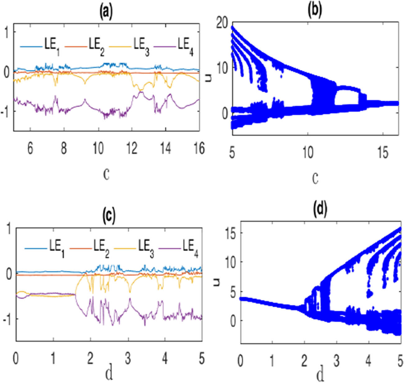
LE and BD of model (1.2) with the same initial values as Figure 1: (a) LE for parameters
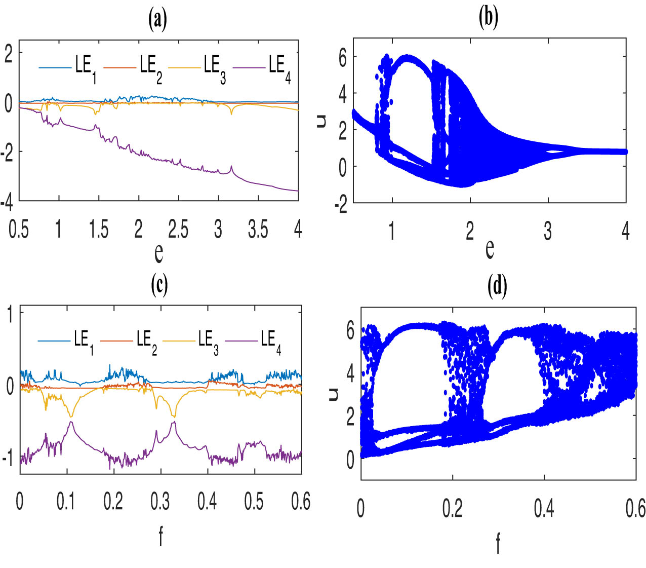
LE and BD of model (1.2) with the same initial values as Figure 1: (a) LE for parameters
LE and BD of model (1.2) with the same initial values as Figure 1: (a) LE for parameters
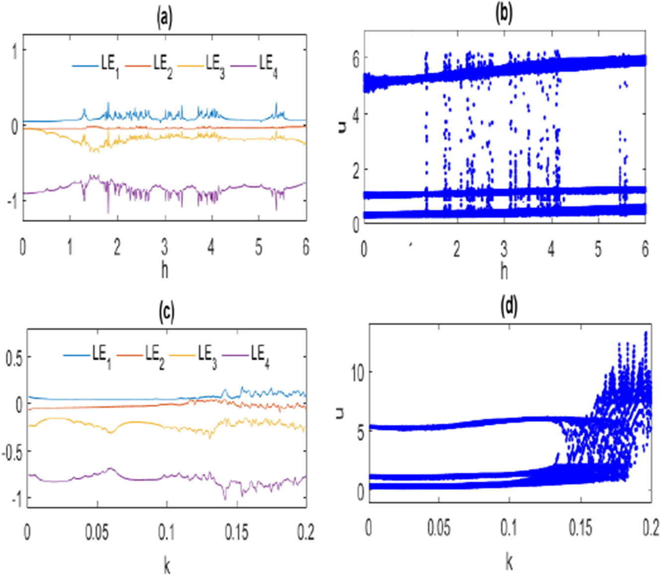
2.5 Dynamics of model (1.2) with equilibrium points
Regarding the selection
The LEs and BDs for the proposed hyperchaotic (chaotic) model (1.2) are provided for the same initial values in Figure 1, and the parameter values are
Fix
LE and BD of model (1.2) with the same initial values as Figure 1: (a) LE for parameters
Fix
By a similar way, the LEs and BDs for the reminder parameters of model (1.2) can be presented for this case.
3 Circuit implementation of model (1.2)
Examining equations of model (1.2) with
We can implement the electronic circuit in Figure 8 using model (3.1), and the circuit equations in the Laplace domain are shown as
where
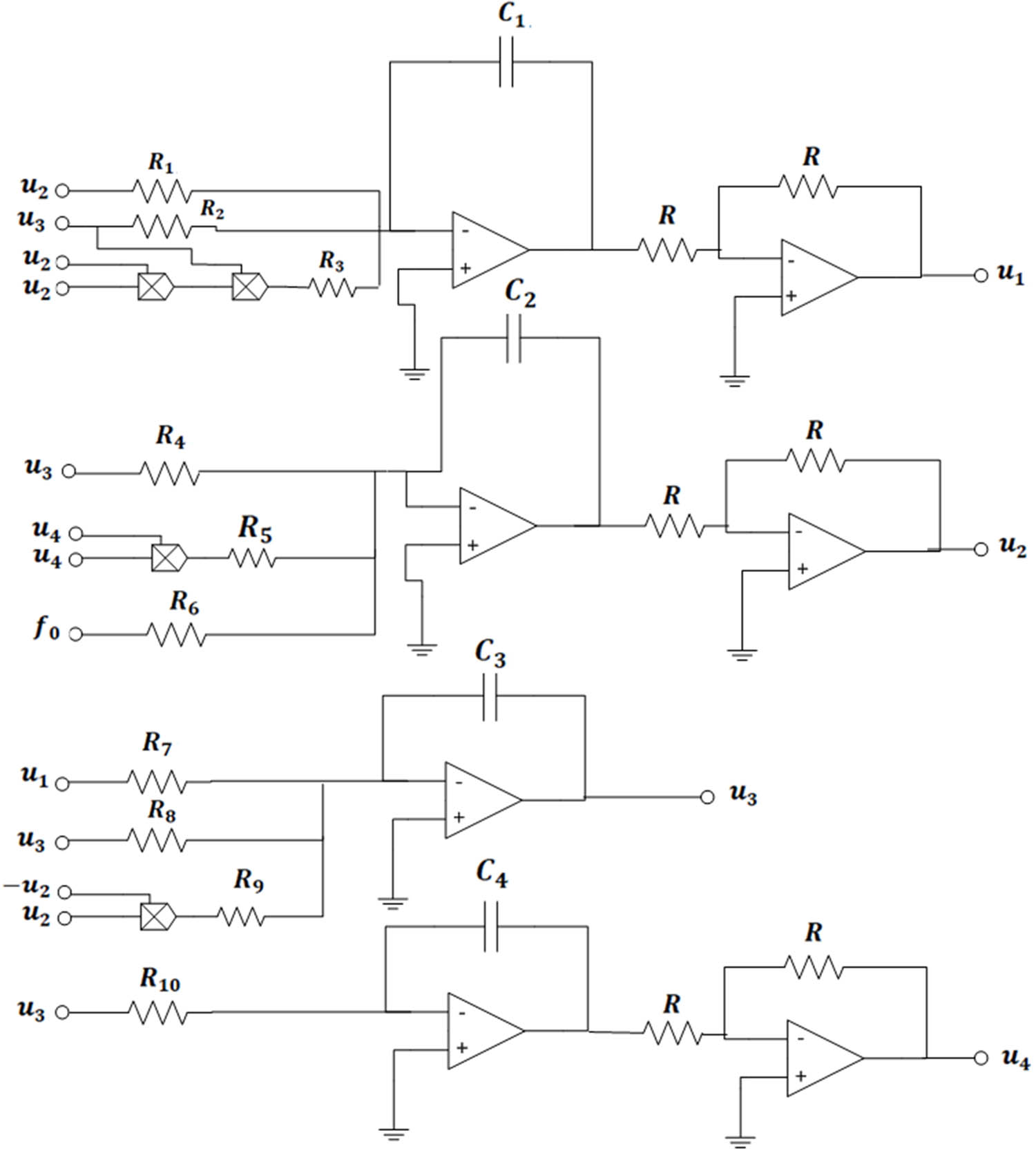
Circuit diagram of model (3.1).
On the MATLAB Simulink, the circuit implementation and simulations were performed. The observed circuit simulations of the chaotic system (3.1) in the
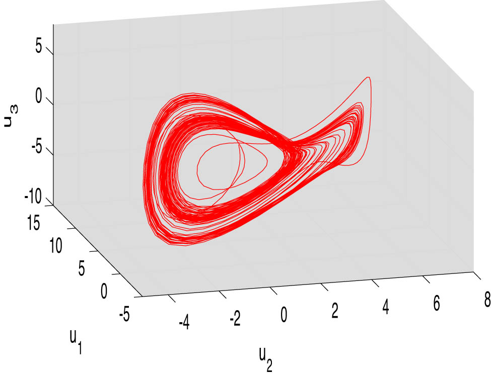
Circuit simulation of model (3.1) in the
Circuit simulation of model (3.1) in the
4 Color image encryption using the hyperchaotic model (1.2)
Using the hyperchaotic model (1.2), the encryption and decryption process [41] entails a number of systematic steps to guarantee secure image transformation. Image preparation is the first step in the process, during which the color image is read and adjusted for further processing. Chaotic sequences are then generated using model (1.2) parameters and initial values, discretizing time for iterative calculations that create hyperchaotic sequences aligned with pixel positions. Channel-wise encryption follows, dividing the image into red, green, blue (color model) (RGB) channels and adjusting the chaotic sequences for each channel before applying encryption through simple addition and wrapping operations. Decryption reverses this process by subtracting the chaotic sequence and restoring the original pixel values. Image reconstruction merges decrypted channels to form the complete image.
In the experimental results, we utilize identical parameter values and initial values for model (1.2), as shown in Figure 1, along with the “House” image to evaluate the effectiveness of the image encryption technique. The original medical image, the encrypted one, and the decrypted image are shown in Figure 11. Figure 11(a)–(c) demonstrates how the encrypted image becomes unreadable during encryption and looks entirely different from the decrypted image. However, when visually compared, the original image and its decrypted version appear exactly the same.
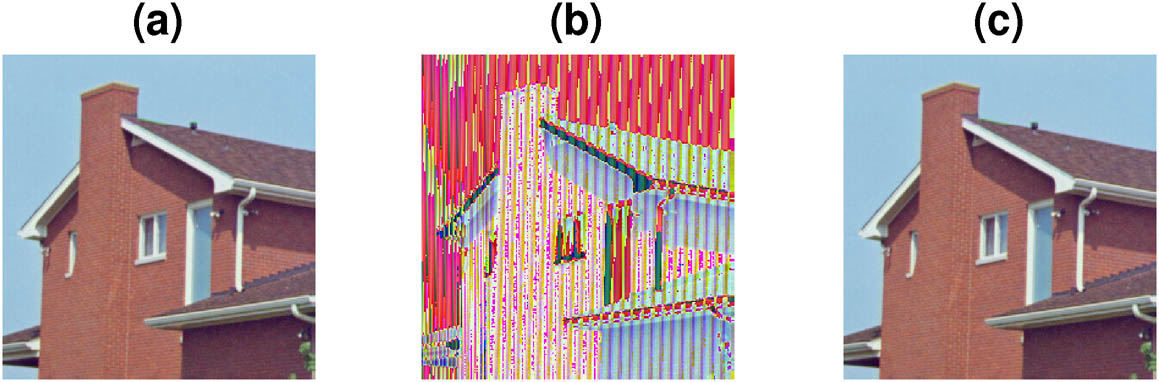
Color image encryption of the “House” image using the hyperchaotic model (1.2): (a) the original image, (b) the encrypted image, and (c) the decrypted image.
Figure 11(a)–(c) shows that the red component of the encrypted image has a different histogram compared to the original and decrypted images. Similarly, Figure 11(d)–(f) displays differences in the green component, and Figure 11(g)–(i) shows changes in the blue component. This makes it hard for attackers to extract useful information or use statistical tools to figure out the original image.
The original “House” image has an information entropy of 7.0686, which indicates that the distribution of its pixels is very unpredictable. Following encryption, the entropy increases to 7.9970, which is close to the maximum value of 8 for an 8-bit image. This suggests that the encrypted image is extremely safe and disordered. After decryption, the entropy goes back to 7.0686, which corresponds to the original image and validates that the image was successfully recovered without any information being lost.
The original “House” image has a correlation coefficient of 0.9840, which shows that adjacent pixels are strongly correlated. The coefficient decreases to
The NPCR for the encrypted “House” image is 100, indicating that 100% of the pixels have changed compared to the original image. This demonstrates the high sensitivity of the encryption process, ensuring strong security against differential attacks.
The encrypted “House” image has a UACI of 29.1854, meaning that there is an average intensity difference of about 29.19% between the original and encrypted photos. This value further validates the efficiency of the encryption process in reaching a high degree of security since it shows a notable change in pixel values.
While our encryption scheme demonstrates strong performance in NPCR (100%) and UACI (29%), we acknowledge that a complete cryptographic evaluation requires additional security analyses. In future work, we will conduct key sensitivity analysis with finer perturbations, evaluate resistance to known/chosen-plaintext attacks, perform key space analysis with formal entropy measurements, and benchmark against state-of-the-art chaos-based methods. These tests will further validate the robustness of our hyperchaos-driven encryption for real-world applications.
5 Conclusion
A new 4D hyperchaotic model is proposed that can produce hidden attractors or self-excited attractors depending on the value of model parameters. For the new 4-DHM model (1.2), some basic dynamical behaviors are investigated. LEs, phase portraits, and BDs have all been used to illustrate the new 4-DHM model’s complicated dynamical characteristics. Remarks 2.1–2.3 show the differences between the new 4-DHM model (1.2) and previous work. For the new 4-DHM model (1.2), an electronic circuit is designed. We think that our proposed model (1.2) is expected to find widespread use in a variety of physics, engineering, and computer science domains, including secure communication, information science, and laser systems. Figure 8 shows the electronic implementation of model (3.1). The simulation observations of our new electronic circuit of the new 4-DHM model (3.1) and those of numerical calculations were in good agreement, as illustrated in Figures 1–6 and 9–10. The encryption, decryption, histogram analysis, information entropy, correlation coefficient, NPCR, and UACI of the color (“House”) image are illustrated using the 4-DHM (1.2), and the results are depicted in Figures 11 and 12.
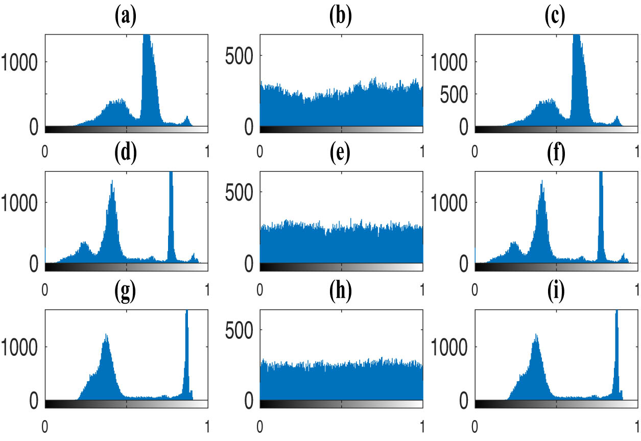
Histogram of color image encryption of the “House” image using the 4-DHM (1.2): (a) the histogram of the red component of the original image, (b) the histogram of the red component of the encrypted image, (c) the histograms of the red component of the decrypted image, (d)–(f) the histograms of the green components, and (g)–(i) the histograms of the blue components.
-
Funding information: The authors extend their appreciation to Prince Sattam bin Abdulaziz University for funding this research work through the Project Number (PSAU/2024/01/31725).
-
Author contributions: The study’s conception and design involved contributions from all authors. TMA wrote the initial draft of the manuscript. MEA conducted material preparation, data collection, and analysis. Through multiple iterations of manuscript revision, each author provided valuable insights and suggestions. The final version of the manuscript was reviewed thoroughly by all authors and unanimously approved for publication.
-
Conflict of interest: The authors state no conflict of interest.
-
Data availability statement: The datasets of the current study are available from the corresponding author on reasonable request.
References
[1] Lorenz EN. Deterministic nonperiodic flow. J Atmos Sci. 1963;20(2):130–41. 10.1175/1520-0469(1963)020<0130:DNF>2.0.CO;2Search in Google Scholar
[2] Heltberg ML, Krishna S, Jensen MH. On chaotic dynamics in transcription factors and the associated effects in differential gene regulation. Nat Commun. 2019;10(1):71. 10.1038/s41467-018-07932-1Search in Google Scholar
[3] Dharminder D, Kumar U, Gupta P. A construction of a conformal Chebyshev chaotic map based authentication protocol for healthcare telemedicine services. Complex Intell Syst. 2021;7(5):2531–42. 10.1007/s40747-021-00441-7Search in Google Scholar
[4] Li X, Jiang C, Xu R, Yang W, Wang H, Zou Y. Combining forecast of landslide displacement based on chaos theory. Arab J Geosci. 2021;14:1–10. 10.1007/s12517-021-06514-8Search in Google Scholar
[5] Mahmoud GM, Farghaly AA, Abed-Elhameed TM, Darwish MM. Adaptive dual synchronization of chaotic (hyperchaotic) complex systems with uncertain parameters and its application in image encryption. Acta Phys Polonica B. 2018;49(11):1923. 10.5506/APhysPolB.49.1923Search in Google Scholar
[6] Mahmoud GM, Bountis T, AbdEl-Latif G, Mahmoud EE. Chaos synchronization of two different chaotic complex Chen and Lü systems. Nonl Dyn. 2009;55:43–53. 10.1007/s11071-008-9343-5Search in Google Scholar
[7] Liao Y, Vikram A, Galitski V. Many-body level statistics of single-particle quantum chaos. Phys Rev Let. 2020;125(25):250601. 10.1103/PhysRevLett.125.250601Search in Google Scholar
[8] Awad E, Samir N. A closed-form solution for thermally induced affine deformation in unbounded domains with a temporally accelerated anomalous thermal conductivity. J Phys A Math Theoret. 2024;57(45):455202. 10.1088/1751-8121/ad878fSearch in Google Scholar
[9] Awad E. Modeling of anomalous thermal conduction in thermoelectric magnetohydrodynamics: Couette formulation with a multiphase pressure gradient. Phys Fluids. 2024;36(3):033608. 10.1063/5.0190970Search in Google Scholar
[10] Benkouider K, Sambas A, Bonny T, Al Nassan W, Moghrabi IA, Sulaiman IM, et al. A comprehensive study of the novel 4D hyperchaotic system with self-exited multistability and application in the voice encryption. Scientif Reports. 2024;14(1):12993. 10.1038/s41598-024-63779-1Search in Google Scholar
[11] Rössler OE. An equation for continuous chaos. Phys Lett A. 1976;57(5):397–8. 10.1016/0375-9601(76)90101-8Search in Google Scholar
[12] Matsumoto T. A chaotic attractor from Chuaas circuit. IEEE Trans Circuits Syst. 1984;31(12):1055–8. 10.1109/TCS.1984.1085459Search in Google Scholar
[13] Sprott JC. Some simple chaotic flows. Phys Rev E. 1994;50(2):R647. 10.1103/PhysRevE.50.R647Search in Google Scholar
[14] Chen G, Ueta T. Yet another chaotic attractor. Int J Bifurcat Chaos. 1999;9(7):1465–6. 10.1142/S0218127499001024Search in Google Scholar
[15] Zhu H, Ge J, Qi W, Zhang X, Lu X. Dynamic analysis and image encryption application of a sinusoidal-polynomial composite chaotic system. Math Comput Simulat. 2022;198:188–210. 10.1016/j.matcom.2022.02.029Search in Google Scholar
[16] Abed-Elhameed TM, Otefy M, Mahmoud GM. Dynamics of chaotic and hyperchaotic modified nonlinear Schrödinger equations and their compound synchronization. Phys Scr. 2024 Apr;99(5):055226. 10.1088/1402-4896/ad36edSearch in Google Scholar
[17] Laarem G. A new 4-D hyper chaotic system generated from the 3-D Rösslor chaotic system, dynamical analysis, chaos stabilization via an optimized linear feedback control, it’s fractional order model and chaos synchronization using optimized fractional order sliding mode control. Chaos Solitons Fractals. 2021;152:111437. 10.1016/j.chaos.2021.111437Search in Google Scholar
[18] Xiu C, Fang J, Liu Y. Design and circuit implementation of a novel 5D memristive CNN hyperchaotic system. Chaos Solitons Fractals. 2022;158:112040. 10.1016/j.chaos.2022.112040Search in Google Scholar
[19] Mahmoud GM, Abed-Elhameed TM, Khalaf H. Synchronization of hyperchaotic dynamical systems with different dimensions. Phys Scr. 2021;96(12):125244. 10.1088/1402-4896/ac3152Search in Google Scholar
[20] Guo Q, Wang N, Zhang G. A novel four-element RCLM hyperchaotic circuit based on current-controlled extended memristor. AEU-Int J Electron Commun. 2022;156:154391. 10.1016/j.aeue.2022.154391Search in Google Scholar
[21] Nguenjou LN, Kom G, Pone JM, Kengne J, Tiedeu A. A window of multistability in Genesio-Tesi chaotic system, synchronization and application for securing information. AEU-Int J Electron Commun. 2019;99:201–14. 10.1016/j.aeue.2018.11.033Search in Google Scholar
[22] Vaidyanathan S, Volos C. Advances and applications in chaotic systems. Vol. 636. Berlin, Germany: Springer; 2016. 10.1007/978-3-319-30279-9Search in Google Scholar
[23] Al Themairi A, Mahmoud GM, Farghaly AA, Abed-Elhameed TM. Complex Rayleigh-van-der-Pol-Duffing oscillators: dynamics, phase, antiphase synchronization, and image encryption. Fractal Fract. 2023;7(12):886. 10.3390/fractalfract7120886Search in Google Scholar
[24] Abed-Elhameed TM, Mahmoud GM, Elbadry MM, Ahmed ME. Nonlinear distributed-order models: Adaptive synchronization, image encryption and circuit implementation. Chaos Solitons Fractals. 2023;175:114039. 10.1016/j.chaos.2023.114039Search in Google Scholar
[25] Chai X, Tang Z, Gan Z, Lu Y, Wang B, Zhang Y. SE-NDEND: A novel symmetric watermarking framework with neural network-based chaotic encryption for Internet of medical things. Biomed Signal Proces Control. 2024;90:105877. 10.1016/j.bspc.2023.105877Search in Google Scholar
[26] Mahmoud GM, Khalaf H, Darwish MM, Abed-Elhameed TM. On the fractional-order simplified Lorenz models: Dynamics, synchronization, and medical image encryption. Math Meth Appl Sci. 2023;46(14):15706–25. 10.1002/mma.9422Search in Google Scholar
[27] Dou G, Guo W, Li Z, Wang C. Dynamics analysis of memristor chaotic circuit with coexisting hidden attractors. Europ Phys J Plus. 2024;139(4):1–17. 10.1140/epjp/s13360-024-05140-zSearch in Google Scholar
[28] Shilnikov LP. A case of the existence of a denumerable set of periodic motions. Sov Math Dokl. 1965;6:163–6. Search in Google Scholar
[29] Leonov G, Kuznetsov N, Mokaev T. Homoclinic orbits, and self-excited and hidden attractors in a Lorenz-like system describing convective fluid motion: Homoclinic orbits, and self-excited and hidden attractors. Europ Phys J Special Topics. 2015;224:1421–58. 10.1140/epjst/e2015-02470-3Search in Google Scholar
[30] Leonov GA, Kuznetsov NV, Mokaev TN. Hidden attractor and homoclinic orbit in Lorenz-like system describing convective fluid motion in rotating cavity. Commun Nonl Sci Numer Simulat. 2015;28(1–3):166–74. 10.1016/j.cnsns.2015.04.007Search in Google Scholar
[31] Sharma P, Shrimali M, Prasad A, Kuznetsov N, Leonov G. Control of multistability in hidden attractors. Europ Phys J Special Topics. 2015;224:1485–91. 10.1140/epjst/e2015-02474-ySearch in Google Scholar
[32] Abed-Elhameed TM, Mahmoud GM, Ahmed ME. On real and complex dynamical models with hidden attractors and their synchronization. Phys Scr. 2023;98(4):045223. 10.1088/1402-4896/acc490Search in Google Scholar
[33] Chua L, Komuro M, Matsumoto T. The double scroll family. IEEE Trans Circuits Syst. 1986;33(11):1072–118. 10.1109/TCS.1986.1085869Search in Google Scholar
[34] Lai Q, Bao B, Chen C, Kengne J, Akgul A. Circuit application of chaotic systems: modeling, dynamical analysis and control. Eur Phys J Special Topics. 2021;230:1691–4. 10.1140/epjs/s11734-021-00202-0Search in Google Scholar
[35] Gao T, Chen G, Chen Z, Cang S. The generation and circuit implementation of a new hyper-chaos based upon Lorenz system. Phys Lett A. 2007;361(1–2):78–86. 10.1016/j.physleta.2006.09.042Search in Google Scholar
[36] Ablay G. Novel chaotic delay systems and electronic circuit solutions. Nonl Dyn. 2015;81(4):1795–804. 10.1007/s11071-015-2107-0Search in Google Scholar
[37] Masood F, Masood J, Zhang L, Jamal SS, Boulila W, Rehman SU, et al. A new color image encryption technique using DNA computing and Chaos-based substitution box. Soft Comput. 2022;26:7461–77. 10.1007/s00500-021-06459-wSearch in Google Scholar
[38] Biban G, Chugh R, Panwar A. Image encryption based on 8D hyperchaotic system using Fibonacci Q-Matrix. Chaos Solitons Fractals. 2023;170:113396. 10.1016/j.chaos.2023.113396Search in Google Scholar
[39] Yan X, Hu Q, Teng L. A novel color image encryption method based on new three-dimensional chaotic mapping and DNA coding. Nonl Dyn. 2025;113(2):1799–826. 10.1007/s11071-024-10277-8Search in Google Scholar
[40] Hu C, Tian Z, Wang Q, Zhang X, Liang B, Jian C, et al. A memristor-based VB2 chaotic system: Dynamical analysis, circuit implementation, and image encryption. Optik. 2022;269:169878. 10.1016/j.ijleo.2022.169878Search in Google Scholar
[41] Guan ZH, Huang F, Guan W. Chaos-based image encryption algorithm. Phys Let A. 2005;346(1–3):153–7. 10.1016/j.physleta.2005.08.006Search in Google Scholar
© 2025 the author(s), published by De Gruyter
This work is licensed under the Creative Commons Attribution 4.0 International License.
Articles in the same Issue
- Research Articles
- Single-step fabrication of Ag2S/poly-2-mercaptoaniline nanoribbon photocathodes for green hydrogen generation from artificial and natural red-sea water
- Abundant new interaction solutions and nonlinear dynamics for the (3+1)-dimensional Hirota–Satsuma–Ito-like equation
- A novel gold and SiO2 material based planar 5-element high HPBW end-fire antenna array for 300 GHz applications
- Explicit exact solutions and bifurcation analysis for the mZK equation with truncated M-fractional derivatives utilizing two reliable methods
- Optical and laser damage resistance: Role of periodic cylindrical surfaces
- Numerical study of flow and heat transfer in the air-side metal foam partially filled channels of panel-type radiator under forced convection
- Water-based hybrid nanofluid flow containing CNT nanoparticles over an extending surface with velocity slips, thermal convective, and zero-mass flux conditions
- Dynamical wave structures for some diffusion--reaction equations with quadratic and quartic nonlinearities
- Solving an isotropic grey matter tumour model via a heat transfer equation
- Study on the penetration protection of a fiber-reinforced composite structure with CNTs/GFP clip STF/3DKevlar
- Influence of Hall current and acoustic pressure on nanostructured DPL thermoelastic plates under ramp heating in a double-temperature model
- Applications of the Belousov–Zhabotinsky reaction–diffusion system: Analytical and numerical approaches
- AC electroosmotic flow of Maxwell fluid in a pH-regulated parallel-plate silica nanochannel
- Interpreting optical effects with relativistic transformations adopting one-way synchronization to conserve simultaneity and space–time continuity
- Modeling and analysis of quantum communication channel in airborne platforms with boundary layer effects
- Theoretical and numerical investigation of a memristor system with a piecewise memductance under fractal–fractional derivatives
- Tuning the structure and electro-optical properties of α-Cr2O3 films by heat treatment/La doping for optoelectronic applications
- High-speed multi-spectral explosion temperature measurement using golden-section accelerated Pearson correlation algorithm
- Dynamic behavior and modulation instability of the generalized coupled fractional nonlinear Helmholtz equation with cubic–quintic term
- Study on the duration of laser-induced air plasma flash near thin film surface
- Exploring the dynamics of fractional-order nonlinear dispersive wave system through homotopy technique
- The mechanism of carbon monoxide fluorescence inside a femtosecond laser-induced plasma
- Numerical solution of a nonconstant coefficient advection diffusion equation in an irregular domain and analyses of numerical dispersion and dissipation
- Numerical examination of the chemically reactive MHD flow of hybrid nanofluids over a two-dimensional stretching surface with the Cattaneo–Christov model and slip conditions
- Impacts of sinusoidal heat flux and embraced heated rectangular cavity on natural convection within a square enclosure partially filled with porous medium and Casson-hybrid nanofluid
- Stability analysis of unsteady ternary nanofluid flow past a stretching/shrinking wedge
- Solitonic wave solutions of a Hamiltonian nonlinear atom chain model through the Hirota bilinear transformation method
- Bilinear form and soltion solutions for (3+1)-dimensional negative-order KdV-CBS equation
- Solitary chirp pulses and soliton control for variable coefficients cubic–quintic nonlinear Schrödinger equation in nonuniform management system
- Influence of decaying heat source and temperature-dependent thermal conductivity on photo-hydro-elasto semiconductor media
- Dissipative disorder optimization in the radiative thin film flow of partially ionized non-Newtonian hybrid nanofluid with second-order slip condition
- Bifurcation, chaotic behavior, and traveling wave solutions for the fractional (4+1)-dimensional Davey–Stewartson–Kadomtsev–Petviashvili model
- New investigation on soliton solutions of two nonlinear PDEs in mathematical physics with a dynamical property: Bifurcation analysis
- Mathematical analysis of nanoparticle type and volume fraction on heat transfer efficiency of nanofluids
- Creation of single-wing Lorenz-like attractors via a ten-ninths-degree term
- Optical soliton solutions, bifurcation analysis, chaotic behaviors of nonlinear Schrödinger equation and modulation instability in optical fiber
- Chaotic dynamics and some solutions for the (n + 1)-dimensional modified Zakharov–Kuznetsov equation in plasma physics
- Fractal formation and chaotic soliton phenomena in nonlinear conformable Heisenberg ferromagnetic spin chain equation
- Single-step fabrication of Mn(iv) oxide-Mn(ii) sulfide/poly-2-mercaptoaniline porous network nanocomposite for pseudo-supercapacitors and charge storage
- Novel constructed dynamical analytical solutions and conserved quantities of the new (2+1)-dimensional KdV model describing acoustic wave propagation
- Tavis–Cummings model in the presence of a deformed field and time-dependent coupling
- Spinning dynamics of stress-dependent viscosity of generalized Cross-nonlinear materials affected by gravitationally swirling disk
- Design and prediction of high optical density photovoltaic polymers using machine learning-DFT studies
- Robust control and preservation of quantum steering, nonlocality, and coherence in open atomic systems
- Coating thickness and process efficiency of reverse roll coating using a magnetized hybrid nanomaterial flow
- Dynamic analysis, circuit realization, and its synchronization of a new chaotic hyperjerk system
- Decoherence of steerability and coherence dynamics induced by nonlinear qubit–cavity interactions
- Finite element analysis of turbulent thermal enhancement in grooved channels with flat- and plus-shaped fins
- Modulational instability and associated ion-acoustic modulated envelope solitons in a quantum plasma having ion beams
- Statistical inference of constant-stress partially accelerated life tests under type II generalized hybrid censored data from Burr III distribution
- On solutions of the Dirac equation for 1D hydrogenic atoms or ions
- Entropy optimization for chemically reactive magnetized unsteady thin film hybrid nanofluid flow on inclined surface subject to nonlinear mixed convection and variable temperature
- Stability analysis, circuit simulation, and color image encryption of a novel four-dimensional hyperchaotic model with hidden and self-excited attractors
- A high-accuracy exponential time integration scheme for the Darcy–Forchheimer Williamson fluid flow with temperature-dependent conductivity
- Novel analysis of fractional regularized long-wave equation in plasma dynamics
- Development of a photoelectrode based on a bismuth(iii) oxyiodide/intercalated iodide-poly(1H-pyrrole) rough spherical nanocomposite for green hydrogen generation
- Investigation of solar radiation effects on the energy performance of the (Al2O3–CuO–Cu)/H2O ternary nanofluidic system through a convectively heated cylinder
- Quantum resources for a system of two atoms interacting with a deformed field in the presence of intensity-dependent coupling
- Studying bifurcations and chaotic dynamics in the generalized hyperelastic-rod wave equation through Hamiltonian mechanics
- A new numerical technique for the solution of time-fractional nonlinear Klein–Gordon equation involving Atangana–Baleanu derivative using cubic B-spline functions
- Interaction solutions of high-order breathers and lumps for a (3+1)-dimensional conformable fractional potential-YTSF-like model
- Hydraulic fracturing radioactive source tracing technology based on hydraulic fracturing tracing mechanics model
- Numerical solution and stability analysis of non-Newtonian hybrid nanofluid flow subject to exponential heat source/sink over a Riga sheet
- Numerical investigation of mixed convection and viscous dissipation in couple stress nanofluid flow: A merged Adomian decomposition method and Mohand transform
- Effectual quintic B-spline functions for solving the time fractional coupled Boussinesq–Burgers equation arising in shallow water waves
- Analysis of MHD hybrid nanofluid flow over cone and wedge with exponential and thermal heat source and activation energy
- Solitons and travelling waves structure for M-fractional Kairat-II equation using three explicit methods
- Impact of nanoparticle shapes on the heat transfer properties of Cu and CuO nanofluids flowing over a stretching surface with slip effects: A computational study
- Computational simulation of heat transfer and nanofluid flow for two-sided lid-driven square cavity under the influence of magnetic field
- Irreversibility analysis of a bioconvective two-phase nanofluid in a Maxwell (non-Newtonian) flow induced by a rotating disk with thermal radiation
- Hydrodynamic and sensitivity analysis of a polymeric calendering process for non-Newtonian fluids with temperature-dependent viscosity
- Exploring the peakon solitons molecules and solitary wave structure to the nonlinear damped Kortewege–de Vries equation through efficient technique
- Modeling and heat transfer analysis of magnetized hybrid micropolar blood-based nanofluid flow in Darcy–Forchheimer porous stenosis narrow arteries
- Activation energy and cross-diffusion effects on 3D rotating nanofluid flow in a Darcy–Forchheimer porous medium with radiation and convective heating
- Insights into chemical reactions occurring in generalized nanomaterials due to spinning surface with melting constraints
- Influence of a magnetic field on double-porosity photo-thermoelastic materials under Lord–Shulman theory
- Soliton-like solutions for a nonlinear doubly dispersive equation in an elastic Murnaghan's rod via Hirota's bilinear method
- Analytical and numerical investigation of exact wave patterns and chaotic dynamics in the extended improved Boussinesq equation
- Nonclassical correlation dynamics of Heisenberg XYZ states with (x, y)-spin--orbit interaction, x-magnetic field, and intrinsic decoherence effects
- Exact traveling wave and soliton solutions for chemotaxis model and (3+1)-dimensional Boiti–Leon–Manna–Pempinelli equation
- Unveiling the transformative role of samarium in ZnO: Exploring structural and optical modifications for advanced functional applications
- On the derivation of solitary wave solutions for the time-fractional Rosenau equation through two analytical techniques
- Analyzing the role of length and radius of MWCNTs in a nanofluid flow influenced by variable thermal conductivity and viscosity considering Marangoni convection
- Advanced mathematical analysis of heat and mass transfer in oscillatory micropolar bio-nanofluid flows via peristaltic waves and electroosmotic effects
- Exact bound state solutions of the radial Schrödinger equation for the Coulomb potential by conformable Nikiforov–Uvarov approach
- Some anisotropic and perfect fluid plane symmetric solutions of Einstein's field equations using killing symmetries
- Nonlinear dynamics of the dissipative ion-acoustic solitary waves in anisotropic rotating magnetoplasmas
- Curves in multiplicative equiaffine plane
- Exact solution of the three-dimensional (3D) Z2 lattice gauge theory
- Propagation properties of Airyprime pulses in relaxing nonlinear media
- Symbolic computation: Analytical solutions and dynamics of a shallow water wave equation in coastal engineering
- Wave propagation in nonlocal piezo-photo-hygrothermoelastic semiconductors subjected to heat and moisture flux
- Comparative reaction dynamics in rotating nanofluid systems: Quartic and cubic kinetics under MHD influence
- Laplace transform technique and probabilistic analysis-based hypothesis testing in medical and engineering applications
- Physical properties of ternary chloro-perovskites KTCl3 (T = Ge, Al) for optoelectronic applications
- Gravitational length stretching: Curvature-induced modulation of quantum probability densities
- The search for the cosmological cold dark matter axion – A new refined narrow mass window and detection scheme
- A comparative study of quantum resources in bipartite Lipkin–Meshkov–Glick model under DM interaction and Zeeman splitting
- PbO-doped K2O–BaO–Al2O3–B2O3–TeO2-glasses: Mechanical and shielding efficacy
- Nanospherical arsenic(iii) oxoiodide/iodide-intercalated poly(N-methylpyrrole) composite synthesis for broad-spectrum optical detection
- Sine power Burr X distribution with estimation and applications in physics and other fields
- Numerical modeling of enhanced reactive oxygen plasma in pulsed laser deposition of metal oxide thin films
- Dynamical analyses and dispersive soliton solutions to the nonlinear fractional model in stratified fluids
- Computation of exact analytical soliton solutions and their dynamics in advanced optical system
- An innovative approximation concerning the diffusion and electrical conductivity tensor at critical altitudes within the F-region of ionospheric plasma at low latitudes
- An analytical investigation to the (3+1)-dimensional Yu–Toda–Sassa–Fukuyama equation with dynamical analysis: Bifurcation
- Swirling-annular-flow-induced instability of a micro shell considering Knudsen number and viscosity effects
- Numerical analysis of non-similar convection flows of a two-phase nanofluid past a semi-infinite vertical plate with thermal radiation
- MgO NPs reinforced PCL/PVC nanocomposite films with enhanced UV shielding and thermal stability for packaging applications
- Optimal conditions for indoor air purification using non-thermal Corona discharge electrostatic precipitator
- Investigation of thermal conductivity and Raman spectra for HfAlB, TaAlB, and WAlB based on first-principles calculations
- Tunable double plasmon-induced transparency based on monolayer patterned graphene metamaterial
- DSC: depth data quality optimization framework for RGBD camouflaged object detection
- A new family of Poisson-exponential distributions with applications to cancer data and glass fiber reliability
- Numerical investigation of couple stress under slip conditions via modified Adomian decomposition method
- Monitoring plateau lake area changes in Yunnan province, southwestern China using medium-resolution remote sensing imagery: applicability of water indices and environmental dependencies
- Heterodyne interferometric fiber-optic gyroscope
- Exact solutions of Einstein’s field equations via homothetic symmetries of non-static plane symmetric spacetime
- A widespread study of discrete entropic model and its distribution along with fluctuations of energy
- Empirical model integration for accurate charge carrier mobility simulation in silicon MOSFETs
- The influence of scattering correction effect based on optical path distribution on CO2 retrieval
- Anisotropic dissociation and spectral response of 1-Bromo-4-chlorobenzene under static directional electric fields
- Role of tungsten oxide (WO3) on thermal and optical properties of smart polymer composites
- Analysis of iterative deblurring: no explicit noise
- The influence of anisotropy of InP on its elasticity and phonon properties
- Review Article
- Examination of the gamma radiation shielding properties of different clay and sand materials in the Adrar region
- Erratum
- Erratum to “On Soliton structures in optical fiber communications with Kundu–Mukherjee–Naskar model (Open Physics 2021;19:679–682)”
- Special Issue on Fundamental Physics from Atoms to Cosmos - Part II
- Possible explanation for the neutron lifetime puzzle
- Special Issue on Nanomaterial utilization and structural optimization - Part III
- Numerical investigation on fluid-thermal-electric performance of a thermoelectric-integrated helically coiled tube heat exchanger for coal mine air cooling
- Special Issue on Nonlinear Dynamics and Chaos in Physical Systems
- Analysis of the fractional relativistic isothermal gas sphere with application to neutron stars
- Abundant wave symmetries in the (3+1)-dimensional Chafee–Infante equation through the Hirota bilinear transformation technique
- Successive midpoint method for fractional differential equations with nonlocal kernels: Error analysis, stability, and applications
- Novel exact solitons to the fractional modified mixed-Korteweg--de Vries model with a stability analysis