Dynamical wave structures for some diffusion--reaction equations with quadratic and quartic nonlinearities
-
Nauman Ahmed
 ,
Makhdoom Ali
,
Makhdoom Ali

Abstract
This work investigates the quadratic and quartic nonlinear diffusion–reaction equations with nonlinear convective flux terms, which are investigated analytically. Diffusion–reaction equations have a wide range of applications in several scientific areas, such as chemistry, biology, and population dynamics of the species. The new extended direct algebraic method is applied to obtain abundant families of solitary wave solutions. Different types of solitary wave solutions are obtained by applying this analytical method. This approach provides the solutions in the form of single and combined wave structures, which are observed in shock, complex solitary-shock, shock-singular, and periodic-singular forms. Some of the solutions are depicted graphically to illustrate the fact that they are, indeed, wave solutions of the mathematical model.
1 Introduction
In the physical sciences, differential equations (DEs) are essential to describe some physical phenomena. Many important evolutionary occurrences are often modeled by nonlinear partial differential equations (NPDEs). Most physical phenomena in various fields, such as field theory, optical fiber [1,2], mathematical physics, plasma physics [3], biophysics, fluid dynamics, mechanics, aerospace industry [4], chemistry reactions [5–7], metrology, and many other fields [8–10] are described by using the NPDEs. For instance, the nonlinear Schrödinger equation (NLSE) has numerous applications in scientific fields such as nonlinear optics, mathematical finance, plasma physics, nuclear and solid-state physics, biochemistry, superconductivity, and matter.
As most of the physical occurrences are modeled by NPDEs. It is essential to find the solutions to NPDEs. Finding the solutions to the NPDEs is crucial to having a thorough understanding of the phenomenon. To obtain the exact solution, a range of analytical techniques have been developed and reported in the literature. The Kudryashov method [11], the homogenous balance method [12,13], the generalized Kudryashov method [14,15], the tanh–coth method [16,17], the direct algebraic method, extended modified auxiliary equation mapping method, the unified method, the modified and extended rational expansion method, the extended
It is worth pointing out that Yan and Lou worked on the soliton molecules of Sharma–Tasso–Olver–Burgers equation [29], Wu et al. investigated the nonlinear von Karman equations for the three-layer microplates [30]. Meanwhile, Wang et al. considered the diffusively delay-coupled memristive Chialvo neuron map for the network patterns [31], while Dai et al. worked on the macrodispersivity models with an analytical solution [32]. Kai and Yin worked on the Gaussian traveling wave solution to a special kind of Schrödinger equation [33], Zhu et al. used the logarithmic transformation for the modified Schrödinger’s equation [34] and nonlinear Zakharov system [35] to obtain analytical solutions. Berkal and Almatrafi worked on the bifurcation and stability of a two-dimensional activator–inhibitor model [36], and some researchers have worked on the approximate solutions of reaction–diffusion models [37–40]. in the present study, we will derive exact solutions for a nonlinear reaction–diffusion system.
Our current research focuses on nonlinear diffusion–reaction (DR) equations, which have wide applications in biology, chemical, physical, and logical systems. Various reduced versions of the DR equations have been investigated in the literature. In the study by Triki et al. [41], the auxiliary equation method was used to study three nonlinear DR equations in inhomogeneous mediums, including derivative-type and algebraic-type nonlinearities. Furthermore, nonlinear reaction diffusion equations with cubic and quantic nonlinearities, nonlinear DR equations including quadratic-cubic nonlinearities, and nonlinear diffusion–reaction equations with a nonlinear convective flux term have been investigated by Bhardwaj et al. [42], Malik et al. [43,44]. We examine the DR equation for a case where the diffusion coefficient
In the present work, we investigate the dynamics through the solutions of particular nonlinear DR equations, which include a nonlinear convective flux term along with quadratic and biquadratic nonlinearities and are represented by the following equations:
where
The purpose of this study is to improve the accuracy of possible soliton solutions of the DR equations through a new methodology. Being a novel analytical technique, the new extended direct algebraic method (NEDAM) has not been applied to solve nonlinear DR equations with a nonlinear convective flux term. In domains including engineering, physics, and applied mathematics, NEDAM has demonstrated its reliability and effectiveness in resolving NPDEs. For example, Vahidi [45], Mirhosseini-Alizamini et al. [46], and Munawar et al. [47] have used NEDAM to solve different types of NPDEs. Furthermore, Kurt et al. used NEDAM to find traveling and solitary wave solutions of the potential Kadomtsev–Petviashvili equation. The author found that the NEDAM is accurate, effective, and applicable for solving problems. There are many other methods that provided us with hyperbolic, trigonometric, and rational function solutions. As we will see, single and combined wave structures are observed in shock, complex solitary-shock, shock-singular, and periodic-singular forms. Rational solutions also emerged during the derivation.
The present work is organized as follows. Section 2 is devoted to provide a brief summary of the NEDAM. To that end, we employ [48] as a guiding reference. The methodology is explained in its most general setting. We provide therein a set of steps that lead to the derivation of exact traveling-wave solutions of general systems of partial DEs in two variables, namely, space and time. Moreover, various cases are fully described to reach exact solutions for those models. In turn, Section 3 is devoted to derive the exact traveling-wave solutions for the mathematical models (1) and (2). From our discussion, it can be readily checked the existence of abundant solutions of this form for our mathematical models. For the sake of convenience, we illustrate the behavior of just some of those solutions by means of three-dimensional plots, contour plots, and two-dimensional plots. As we can see from the figures, all of the solutions obtained through the NEDAM are traveling waves. Finally, we close this work with a section of concluding remarks.
2 Method
In this section, we provide an outline of the NEDAM [48]. This method consists of the next steps.
Step 1. We suppose that a NLPDE can be expressed as follows:
where
Step 2. Consider the transformation
where
Step 3. We assume that (4) has a solution of the form
where
where
If
(7)(8)(9)(10)(11)where
(12)
If
(13)(14)(15)(16)(17)where
(18)
If
(19)(20)(21)(22)(23)
If
(24)(25)(26)(27)
If
(28)(29)(30)(31)(32)
If
(33)(34)(35)(36)(37)
If
(38)If
If
If
(39)If
(40)(41)If
(42)
where
Step 4. Calculate
Step 5. Combine Eq. (5) together with Eq. (4), set coefficients of
3 Results
The present section is divided into two stages. In Section 3.1, we derive exact solutions for the quadratic model and, Section 3.2, we obtain solutions for the quartic model.
3.1 Quadratic model
To obtain soliton solutions of the DR equations under study in the present work, we employ the traveling-wave transformation
where the prime symbol denotes the order of derivative of the function
By using Eq. (50) and its derivative in Eq. (49) and by equating the coefficient of the powers of
By manipulating Eq. (50) along with the different forms of
When
(55)(56)(57)(58)(59)where
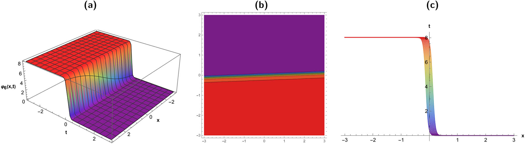
When
(60)(61)(62)(63)(64)Figure 2 shows the graphical behavior of the solution
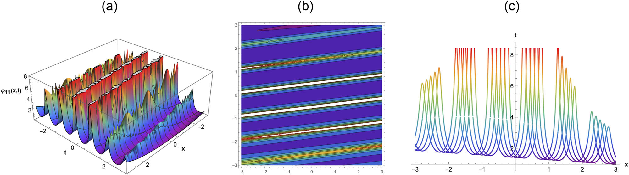
If
(65)(66)(67)(68)(69)Figure 3 shows the graphical behavior of the solution
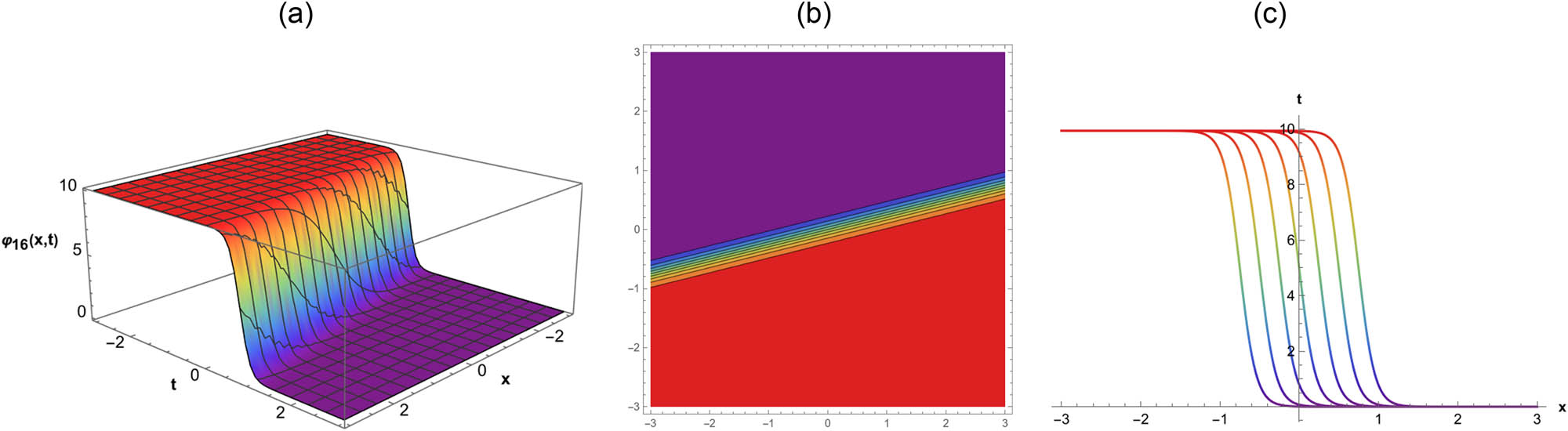
If
(70)(71)(72)(73)(74)For illustration purposes, Figure 4 shows the graphical behavior of the solution
When
(75)(76)(77)(78)(79)
When
(80)(81)(82)(83)(84)
When
(85)If
(86)
When
(87)When
(88)
When
(89)(90)When
(91)
3.2 Quartic model
By applying the traveling wave transformation, we readily obtain the nonlinear ODE
Observe that we obtain that
Family 1.
Family 2.
Proceeding as in the case of the model with quadratic reaction law, we obtain the following traveling wave solutions for Eq. (2).
When
(103)(104)(105)(106)(107)For the sake of convenience, Figure 5 shows graphs of the solution
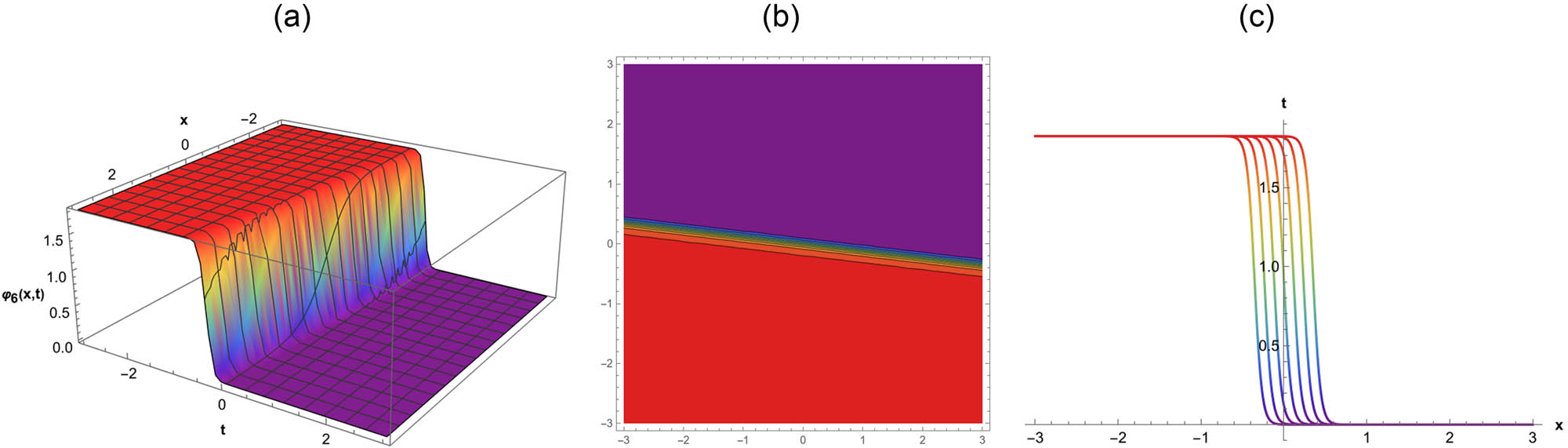
When
(108)(109)(110)(111)(112)For illustration purposes, Figure 6 shows the graphical behavior of the solution
If
(113)(114)(115)(116)(117)
When
(118)(119)(120)(121)(122)Figure 7 shows the solution
If
(123)(124)(125)(126)(127)Figure 8 shows the graphical behavior of the solution
When
(128)(129)(130)(131)(132)
If
(133)When
(134)When
(135)If
(136)
When
(137)(138)If
(139)
4 Discussion
In this section, we will discuss the graphical representation of the results obtained in the previous section by using the new NEDAM. Different types of soliton solutions are seen, including solitary wave, kink, anti-kink, and rational function solutions. Using the Mathematica 11.1 software, graphs have been created to show the solutions physical behavior in the form of 3D, 2D and contour plots. When modeling a variety of physical phenomena (such as chemical reactions, the creation of biological patterns, and heat conduction), reaction–diffusion equations with quadratic and quartic nonlinearities may essential.
It is well known that solitary waves are examples of coherent structures that propagate without distortion because of their limited and stable profiles. The study of energy transfer mechanisms in nonlinear media, including shallow water systems and optical fibers, depends heavily on these waves. Kink and anti-kink solutions, which are frequently used to mimic interfaces or domain walls like those seen in magnetic phase transitions or crystal dislocations, represent monotonic transitions between two stable states. Understanding phase separation and symmetry-breaking dynamics in physical systems requires an understanding of these structures. Less frequently found, rational function solutions describe limited structures with distinctive singular behaviors. These are frequently linked to severe occurrences or anomaly-driven phenomena, such as localized bursts in reaction–diffusion systems or rogue waves in hydrodynamics. Many waveforms and transition patterns are possible due to the interaction between the quadratic and quartic nonlinearities in these equations, which enriches the solution space. Visualizing these solutions offers important information about their stability, dynamics over time and space, and possible uses in systems controlled by complicated pattern generation, phase transitions, and nonlinear energy transfer. In particular, Figure 1 depicts a lump-kink, while Figures 2, 4, and 6 are kink solitons. Figures 3, 5, and 8 provide solitary waves, and Figure 7 shows an anti-kink behavior.

Lump-kink soliton behavior of the solution
Kink soliton behavior of the solution
Solitary wave behavior of the solution
Kink soliton behavior of the solution

Solitary wave behavior of the solution
Kink soliton behavior of the solution
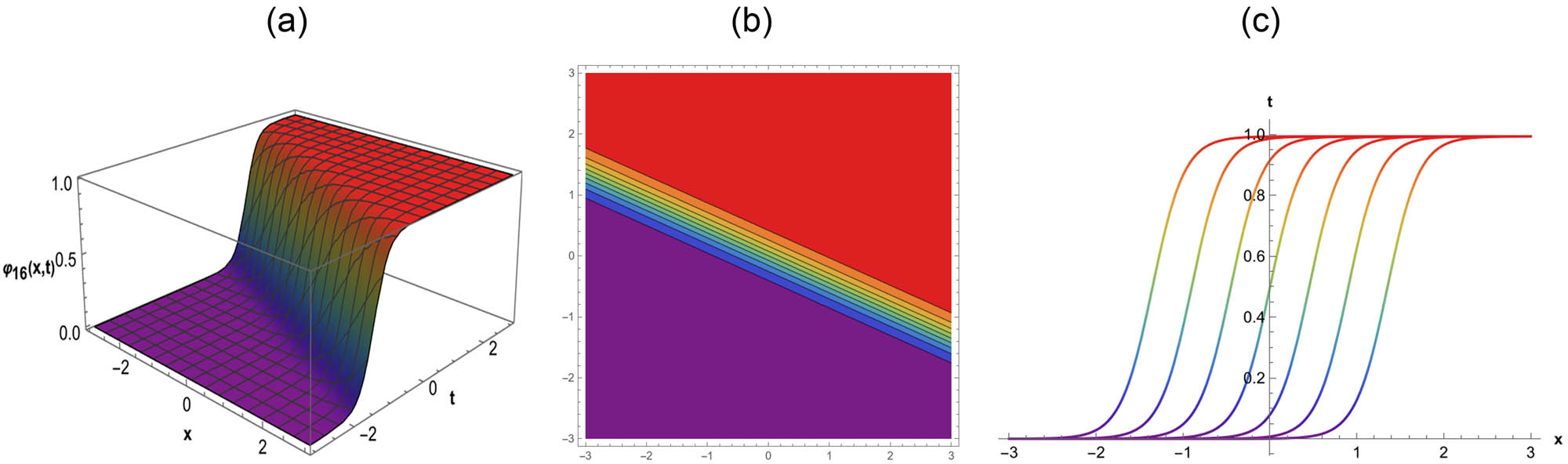
Anti-Kink soliton behavior of the solution
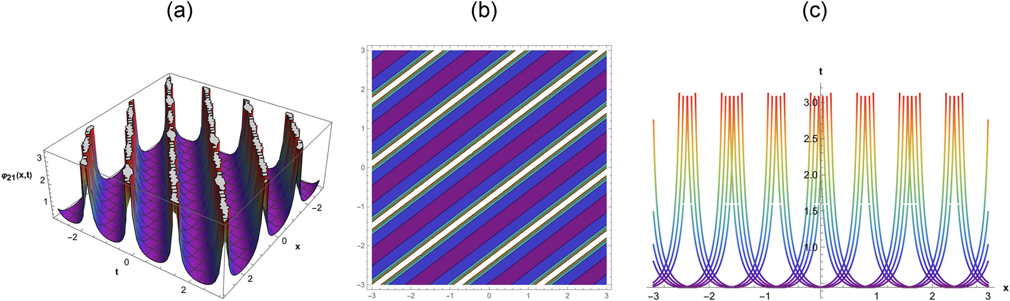
Solitary wave behavior of the solution
5 Conclusions
In this work, the NEDAM has been used to obtain solitary wave solutions for general reaction–diffusion equations with quadratic and quartic nonlinearities. By applying this approach, we have established different types of soliton solutions, including solitary wave, kink, anti-kink, and rational function solutions. To illustrate the physical behavior of the solutions, some plots have been obtained using the Mathematica software. One can obtain various possible results by adjusting the parametric values appropriately. As a conclusion on the side, we have found out that the NEDAM is an appropriate and reliable method for locating precise soliton solutions for broad categories of nonlinear problems. The results obtained in this work were verified by substituting them into the original model equations with the help of Mathematica software. We verified in all cases that the functions derived in this work are actually solutions of our mathematical models. As a future direction of investigation, the models investigated in this work will be extended as NPDEs of higher-order partial differential equations, considering fractional orders of differentiation, and stochastic sources. In those cases, we expect to derive solitary wave solutions by employing the NEDAM, and we will confirm our result numerically through suitable mathematical software.
Acknowledgments
The authors wish to thank the anonymous reviewers for their criticisms. All of their suggestions contributed to improving the quality of this work.
-
Funding information: One of the authors of this work (J.E.M.-D.) wishes to acknowledge the financial support from the National Council of Humanities, Science and Technology of Mexico (CONACYT) through grant A1-S-45928, associated to the research project “Conservative methods for fractional hyperbolic systems: analysis and applications.” In turn, M.G.M.-G. acknowledges the financial support from the program PROSNI of the University of Guadalajara, Mexico.
-
Author contributions: Conceptualization: N.A., J.E.M.-D., M.A., M.J., M.Z.B., M.G.M.-G.; data curation: N.A., J.E.M.-D., M.A., M.J., M.Z.B., M.G.M.-G.; formal analysis: N.A., J.E.M.-D., M.A., M.J., M.Z.B.; funding acquisition: J.E.M.-D., M.G.M.-G.; investigation: N.A., J.E.M.-D., M.A., M.J., M.Z.B., M.G.M.-G.; methodology: N.A., J.E.M.-D., M.A., M.J., M.Z.B., M.G.M.-G.; project administration: J.E.M.-D., M.G.M.-G.; resources: J.E.M.-D., M.G.M.-G.; software: N.A., J.E.M.-D., M.A., M.J., M.Z.B., M.G.M.-G.; supervision: N.A., J.E.M.-D.; validation: N.A., J.E.M.-D., M.A., M.J., M.Z.B., M.G.M.-G.; visualization: N.A., J.E.M.-D., M.A., M.J., M.Z.B., M.G.M.-G.; roles/writing – original draft: N.A., J.E.M.-D., M.A., M.J., M.Z.B., M.G.M.-G.; writing – review editing: N.A., J.E.M.-D., M.A., M.J., M.Z.B., M.G.M.-G. All authors have accepted responsibility for the entire content of this manuscript and approved its submission.
-
Conflict of interest: The authors state no conflict of interest.
-
Data availability statement: All data generated or analysed during this study are included in this published article.
References
[1] Az-Zobi EA, Alomari QM, Afef K, Inc M. Dynamics of generalized time-fractional viscous-capillarity compressible fluid model. Opt Quantum Electron. 2024;56(4):629. 10.1007/s11082-023-06233-2Search in Google Scholar
[2] Fakih H, Faour M, Saoud W, Awad Y. On the complex version of the Cahn-Hilliard-Oono type equation for long interactions phase separation. Int J Math Comput Eng. 2024;2(2):233–59. 10.2478/ijmce-2024-0018Search in Google Scholar
[3] Inc M, Az-Zobi EA, Jhangeer A, Rezazadeh H, Nasir Ali M, Kaabar MK. New soliton solutions for the higher-dimensional non-local Ito equation. Nonlinear Eng. 2021;10(1):374–84. 10.1515/nleng-2021-0029Search in Google Scholar
[4] Az-Zo’bi EA, Al Dawoud K, Marashdeh M. Numeric-analytic solutions of mixed-type systems of balance laws. Appl Math Comput. 2015;265:133–43. 10.1016/j.amc.2015.04.119Search in Google Scholar
[5] Rahman RU, Al-Maaitah AF, Qousini M, Az-Zobi EA, Eldin SM, Abuzar M. New soliton solutions and modulation instability analysis of fractional Huxley equation. Results Phys. 2023;44:106163. 10.1016/j.rinp.2022.106163Search in Google Scholar
[6] Az-Zobi E, Akinyemi L, Alleddawi AO. Construction of optical solitons for conformable generalized model in nonlinear media. Modern Phys Lett B. 2021;35(24):2150409. 10.1142/S0217984921504091Search in Google Scholar
[7] El-Sherif AA, Shoukry MM. Coordination properties of tridentate (N, O, O) heterocyclic alcohol (PDC) with Cu (II): Mixed ligand complex formation reactions of Cu (II) with PDC and some bio-relevant ligands. Spectrochimica Acta Part A Mol Biomol Spectroscopy. 2007;66(3):691–700. 10.1016/j.saa.2006.04.013Search in Google Scholar PubMed
[8] Malik S, Almusawa H, Kumar S, Wazwaz AM, Osman MSA. (2+1)-dimensional Kadomtsev-Petviashvili equation with competing dispersion effect: Painlevé analysis, dynamical behavior and invariant solutions. Results Phys. 2021;23:104043. 10.1016/j.rinp.2021.104043Search in Google Scholar
[9] Shakeel M, Liu X, Mostafa AM, AlQahtani SA, AlQahtani NF, Ali MR. Exploring of soliton solutions in optical metamaterials with parabolic law of nonlinearity. Opt Quantum Electronics. 2024;56(5):860. 10.1007/s11082-024-06452-1Search in Google Scholar
[10] Shakeel M, Liu X, Mostafa AM, AlQahtani NF, Alameri A. Dynamic Solitary Wave Solutions Arising in Nonlinear Chains of Atoms Model. J Nonl Math Phys. 2024;31(1):70. 10.1007/s44198-024-00231-ySearch in Google Scholar
[11] Abdeljabbar A, Roshid HO, Aldurayhim A. Bright, dark, and rogue wave soliton solutions of the quadratic nonlinear Klein-Gordon equation. Symmetry. 2022;14(6):1223. 10.3390/sym14061223Search in Google Scholar
[12] Wang M, Zhou Y, Li Z. Application of a homogeneous balance method to exact solutions of nonlinear equations in mathematical physics. Phys Lett A. 1996;216(1–5):67–75. 10.1016/0375-9601(96)00283-6Search in Google Scholar
[13] Radha B and Duraisamy C. Retracted article: The homogeneous balance method and its applications for finding the exact solutions for nonlinear equations. J Ambient Intel Humanized Comput. 2021;12(6):6591–7. 10.1007/s12652-020-02278-3Search in Google Scholar
[14] Kumar D, Park C, Tamanna N, Paul GC, Osman MS. Dynamics of two-mode Sawada-Kotera equation: Mathematical and graphical analysis of its dual-wave solutions. Results Phys. 2020;19:103581. 10.1016/j.rinp.2020.103581Search in Google Scholar
[15] Rahman MM, Habib MA, Ali HS, Miah MM. The generalized Kudryashov method: a renewed mechanism for performing exact solitary wave solutions of some NLEEs. J Mech Cont Math. 2019;14(1):323–39. 10.26782/jmcms.2019.02.00022Search in Google Scholar
[16] Jabbari A, Kheiri H. New exact traveling wave solutions for the Kawahara and modified Kawahara equations by using modified tanh–coth method. Acta Universitatis Apulensis. 2010;23:21–38. Search in Google Scholar
[17] Bekir A, Cevikel AC. The tanh–coth method combined with the Riccati equation for solving nonlinear coupled equation in mathematical physics. J King Saud Univ-Sci. 2011;23(2):127–32. 10.1016/j.jksus.2010.06.020Search in Google Scholar
[18] Seadawy AR, Alsaedi BA. Dynamical stricture of optical soliton solutions and variational principle of nonlinear Schrödinger equation with Kerr law nonlinearity. Modern Phys Lett B. 2024;38:2450254. 10.1142/S0217984924502543Search in Google Scholar
[19] Seadawy AR, Alsaedi BA. Variational principle and optical soliton solutions for some types of nonlinear Schrödinger dynamical systems. Int J Geometric Meth Modern Phys. 2024;21(6):2430004–245. 10.1142/S0219887824300046Search in Google Scholar
[20] Seadawy AR, Alsaedi BA. Variational principle for generalized unstable and modify unstable nonlinear Schrödinger dynamical equations and their optical soliton solutions. Opt Quantum Electronics. 2024;56(5):844. 10.1007/s11082-024-06417-4Search in Google Scholar
[21] Zhang RF, Bilige S. Bilinear neural network method to obtain the exact analytical solutions of nonlinear partial differential equations and its application to p-gBKP equation. Nonl Dyn. 2019;95:3041–8. 10.1007/s11071-018-04739-zSearch in Google Scholar
[22] Rahman RU, Hammouch Z, Alsubaie ASA, Mahmoud KH, Alshehri A, Az-Zobi EA, et al. Dynamical behavior of fractional nonlinear dispersive equation in Murnaghanas rod materials. Results Phys. 2024;56:107207. 10.1016/j.rinp.2023.107207Search in Google Scholar
[23] Almatrafi MB. Construction of closed form soliton solutions to the space-time fractional symmetric regularized long wave equation using two reliable methods. Fractals. 2023;31(10):2340160. 10.1142/S0218348X23401606Search in Google Scholar
[24] Almatrafi MB. Solitary wave solutions to a fractional model using the improved modified extended tanh-function method. Fractal Fract. 2023;7(3):252. 10.3390/fractalfract7030252Search in Google Scholar
[25] Almatrafi MB, Alharbi A. New soliton wave solutions to a nonlinear equation arising in plasma physics. CMES-Comput Model Eng Sci. 2023;137(1) 827–41. 10.32604/cmes.2023.027344Search in Google Scholar
[26] Alharbi AR, Almatrafi MB. Exact solitary wave and numerical solutions for geophysical KdV equation. J King Saud Univ-Sci. 2022;34(6):102087. 10.1016/j.jksus.2022.102087Search in Google Scholar
[27] Raza N, Osman MS, Abdel-Aty AH, Abdel-Khalek S, Besbes HR. Optical solitons of space-time fractional Fokas-Lenells equation with two versatile integration architectures. Adv Differ Equ. 2020;2020:1–15. 10.1186/s13662-020-02973-7Search in Google Scholar
[28] Shakeel M, Bibi A, Chou D, Zafar A. Study of optical solitons for Kudryashovas Quintuple power-law with dual form of nonlinearity using two modified techniques. Optik. 2023;273:170364. 10.1016/j.ijleo.2022.170364Search in Google Scholar
[29] Yan Z, Lou S. Soliton molecules in Sharma–Tasso–Olver–Burgers equation. Appl Math Lett. 2020;104:106271. 10.1016/j.aml.2020.106271Search in Google Scholar
[30] Wu Q, Wang S, Yao M, Niu Y, Wang C. Nonlinear dynamics of three-layer microplates: simultaneous presence of the micro-scale and imperfect effects. Europ Phys J Plus. 2024;139(5):1–21. 10.1140/epjp/s13360-024-05255-3Search in Google Scholar
[31] Wang Z, Parastesh F, Natiq H, Li J, Xi X, Mehrabbeik M. Synchronization patterns in a network of diffusively delay-coupled memristive Chialvo neuron map. Phys Lett A. 2024;514:129607. 10.1016/j.physleta.2024.129607Search in Google Scholar
[32] Dai Z, Wolfsberg A, Lu Z, Ritzi Jr. R. Representing aquifer architecture in macrodispersivity models with an analytical solution of the transition probability matrix. Geophys Res Lett. 2007;34(20):L20406. 10.1029/2007GL031608Search in Google Scholar
[33] Kai Y, Yin Z. On the Gaussian traveling wave solution to a special kind of Schrödinger equation with logarithmic nonlinearity. Modern Phys Lett B. 2022;36(02):2150543. 10.1142/S0217984921505436Search in Google Scholar
[34] Zhu C, Idris SA, Abdalla MEM, Rezapour S, Shateyi S, Gunay B. Analytical study of nonlinear models using a modified Schrödingeras equation and logarithmic transformation. Results Phys. 2023;55:107183. 10.1016/j.rinp.2023.107183Search in Google Scholar
[35] Zhu C, Al-Dossari M, Rezapour S, Shateyi S, Gunay B. Analytical optical solutions to the nonlinear Zakharov system via logarithmic transformation. Results Phys. 2024;56:107298. 10.1016/j.rinp.2023.107298Search in Google Scholar
[36] Berkal M, Almatrafi MB. Bifurcation and stability of two-dimensional activator–inhibitor model with fractional-order derivative. Fractal Fract. 2023;7(5):344. 10.3390/fractalfract7050344Search in Google Scholar
[37] Sweilam NH, Ahmed SM, Adel M. A simple numerical method for two-dimensional nonlinear fractional anomalous sub-diffusion equations. Math Meth Appl Sci. 2021;44(4):2914–33. 10.1002/mma.6149Search in Google Scholar
[38] Adel M. Numerical simulations for the variable order two-dimensional reaction sub-diffusion equation: Linear and Nonlinear. Fractals. 2022;30(01):2240019. 10.1142/S0218348X22400199Search in Google Scholar
[39] Adel M, Elsaid M. An efficient approach for solving fractional variable order reaction sub-diffusion based on Hermite formula. Fractals. 2022;30(01):2240020. 10.1142/S0218348X22400205Search in Google Scholar
[40] Adel M. Finite difference approach for variable order reaction-subdiffusion equations. Adv Differ Equ. 2018;2018(1):406. 10.1186/s13662-018-1862-xSearch in Google Scholar
[41] Triki H, Leblond H, Mihalache D. Soliton solutions of nonlinear diffusion–reaction-type equations with time-dependent coefficients accounting for long-range diffusion. Nonl Dyn. 2016;86:2115–26. 10.1007/s11071-016-3020-xSearch in Google Scholar
[42] Bhardwaj SB, Singh RM, Sharma K, Mishra SC. Periodic and solitary wave solutions of cubic-quintic nonlinear reaction-diffusion equation with variable convection coefficients. Pramana. 2016;86:1253–8. 10.1007/s12043-015-1177-3Search in Google Scholar
[43] Malik A, Chand F, Kumar H, Mishra SC. Exact solutions of nonlinear diffusion–reaction equations. Indian J Phys. 2012;86(2):129–36. 10.1007/s12648-012-0023-4Search in Google Scholar
[44] Malik A, Kumar H, Chahal RP, Chand F. A dynamical study of certain nonlinear diffusion–reaction equations with a nonlinear convective flux term. Pramana. 2019;92:1–13. 10.1007/s12043-018-1668-0Search in Google Scholar
[45] Vahidi J, Zabihi A, Rezazadeh H, Ansari R. New extended direct algebraic method for the resonant nonlinear Schrödinger equation with Kerr law nonlinearity. Optik. 2021;227:165936. 10.1016/j.ijleo.2020.165936Search in Google Scholar
[46] Mirhosseini-Alizamini SM, Rezazadeh H, Srinivasa K, Bekir A. New closed form solutions of the new coupled Konno-Oono equation using the new extended direct algebraic method. Pramana. 2020;94(1):52. 10.1007/s12043-020-1921-1Search in Google Scholar
[47] Munawar M, Jhangeer A, Pervaiz A, Ibraheem F. New general extended direct algebraic approach for optical solitons of Biswas-Arshed equation through birefringent fibers. Optik. 2021;228:165790. 10.1016/j.ijleo.2020.165790Search in Google Scholar
[48] Bilal M, Ren J, Alsubaie ASA, Mahmoud KH, Inc M. Dynamics of nonlinear diverse wave propagation to Improved Boussinesq model in weakly dispersive medium of shallow waters or ion acoustic waves using efficient technique. Opt Quantum Electron. 2024;56(1):21. 10.1007/s11082-023-05587-xSearch in Google Scholar
© 2025 the author(s), published by De Gruyter
This work is licensed under the Creative Commons Attribution 4.0 International License.
Articles in the same Issue
- Research Articles
- Single-step fabrication of Ag2S/poly-2-mercaptoaniline nanoribbon photocathodes for green hydrogen generation from artificial and natural red-sea water
- Abundant new interaction solutions and nonlinear dynamics for the (3+1)-dimensional Hirota–Satsuma–Ito-like equation
- A novel gold and SiO2 material based planar 5-element high HPBW end-fire antenna array for 300 GHz applications
- Explicit exact solutions and bifurcation analysis for the mZK equation with truncated M-fractional derivatives utilizing two reliable methods
- Optical and laser damage resistance: Role of periodic cylindrical surfaces
- Numerical study of flow and heat transfer in the air-side metal foam partially filled channels of panel-type radiator under forced convection
- Water-based hybrid nanofluid flow containing CNT nanoparticles over an extending surface with velocity slips, thermal convective, and zero-mass flux conditions
- Dynamical wave structures for some diffusion--reaction equations with quadratic and quartic nonlinearities
- Solving an isotropic grey matter tumour model via a heat transfer equation
- Study on the penetration protection of a fiber-reinforced composite structure with CNTs/GFP clip STF/3DKevlar
- Influence of Hall current and acoustic pressure on nanostructured DPL thermoelastic plates under ramp heating in a double-temperature model
- Applications of the Belousov–Zhabotinsky reaction–diffusion system: Analytical and numerical approaches
- AC electroosmotic flow of Maxwell fluid in a pH-regulated parallel-plate silica nanochannel
- Interpreting optical effects with relativistic transformations adopting one-way synchronization to conserve simultaneity and space–time continuity
- Modeling and analysis of quantum communication channel in airborne platforms with boundary layer effects
- Theoretical and numerical investigation of a memristor system with a piecewise memductance under fractal–fractional derivatives
- Tuning the structure and electro-optical properties of α-Cr2O3 films by heat treatment/La doping for optoelectronic applications
- High-speed multi-spectral explosion temperature measurement using golden-section accelerated Pearson correlation algorithm
- Dynamic behavior and modulation instability of the generalized coupled fractional nonlinear Helmholtz equation with cubic–quintic term
- Study on the duration of laser-induced air plasma flash near thin film surface
- Exploring the dynamics of fractional-order nonlinear dispersive wave system through homotopy technique
- The mechanism of carbon monoxide fluorescence inside a femtosecond laser-induced plasma
- Numerical solution of a nonconstant coefficient advection diffusion equation in an irregular domain and analyses of numerical dispersion and dissipation
- Numerical examination of the chemically reactive MHD flow of hybrid nanofluids over a two-dimensional stretching surface with the Cattaneo–Christov model and slip conditions
- Impacts of sinusoidal heat flux and embraced heated rectangular cavity on natural convection within a square enclosure partially filled with porous medium and Casson-hybrid nanofluid
- Stability analysis of unsteady ternary nanofluid flow past a stretching/shrinking wedge
- Solitonic wave solutions of a Hamiltonian nonlinear atom chain model through the Hirota bilinear transformation method
- Bilinear form and soltion solutions for (3+1)-dimensional negative-order KdV-CBS equation
- Solitary chirp pulses and soliton control for variable coefficients cubic–quintic nonlinear Schrödinger equation in nonuniform management system
- Influence of decaying heat source and temperature-dependent thermal conductivity on photo-hydro-elasto semiconductor media
- Dissipative disorder optimization in the radiative thin film flow of partially ionized non-Newtonian hybrid nanofluid with second-order slip condition
- Bifurcation, chaotic behavior, and traveling wave solutions for the fractional (4+1)-dimensional Davey–Stewartson–Kadomtsev–Petviashvili model
- New investigation on soliton solutions of two nonlinear PDEs in mathematical physics with a dynamical property: Bifurcation analysis
- Mathematical analysis of nanoparticle type and volume fraction on heat transfer efficiency of nanofluids
- Creation of single-wing Lorenz-like attractors via a ten-ninths-degree term
- Optical soliton solutions, bifurcation analysis, chaotic behaviors of nonlinear Schrödinger equation and modulation instability in optical fiber
- Chaotic dynamics and some solutions for the (n + 1)-dimensional modified Zakharov–Kuznetsov equation in plasma physics
- Fractal formation and chaotic soliton phenomena in nonlinear conformable Heisenberg ferromagnetic spin chain equation
- Single-step fabrication of Mn(iv) oxide-Mn(ii) sulfide/poly-2-mercaptoaniline porous network nanocomposite for pseudo-supercapacitors and charge storage
- Novel constructed dynamical analytical solutions and conserved quantities of the new (2+1)-dimensional KdV model describing acoustic wave propagation
- Tavis–Cummings model in the presence of a deformed field and time-dependent coupling
- Spinning dynamics of stress-dependent viscosity of generalized Cross-nonlinear materials affected by gravitationally swirling disk
- Design and prediction of high optical density photovoltaic polymers using machine learning-DFT studies
- Robust control and preservation of quantum steering, nonlocality, and coherence in open atomic systems
- Coating thickness and process efficiency of reverse roll coating using a magnetized hybrid nanomaterial flow
- Dynamic analysis, circuit realization, and its synchronization of a new chaotic hyperjerk system
- Decoherence of steerability and coherence dynamics induced by nonlinear qubit–cavity interactions
- Finite element analysis of turbulent thermal enhancement in grooved channels with flat- and plus-shaped fins
- Modulational instability and associated ion-acoustic modulated envelope solitons in a quantum plasma having ion beams
- Statistical inference of constant-stress partially accelerated life tests under type II generalized hybrid censored data from Burr III distribution
- On solutions of the Dirac equation for 1D hydrogenic atoms or ions
- Entropy optimization for chemically reactive magnetized unsteady thin film hybrid nanofluid flow on inclined surface subject to nonlinear mixed convection and variable temperature
- Stability analysis, circuit simulation, and color image encryption of a novel four-dimensional hyperchaotic model with hidden and self-excited attractors
- A high-accuracy exponential time integration scheme for the Darcy–Forchheimer Williamson fluid flow with temperature-dependent conductivity
- Novel analysis of fractional regularized long-wave equation in plasma dynamics
- Development of a photoelectrode based on a bismuth(iii) oxyiodide/intercalated iodide-poly(1H-pyrrole) rough spherical nanocomposite for green hydrogen generation
- Investigation of solar radiation effects on the energy performance of the (Al2O3–CuO–Cu)/H2O ternary nanofluidic system through a convectively heated cylinder
- Quantum resources for a system of two atoms interacting with a deformed field in the presence of intensity-dependent coupling
- Studying bifurcations and chaotic dynamics in the generalized hyperelastic-rod wave equation through Hamiltonian mechanics
- A new numerical technique for the solution of time-fractional nonlinear Klein–Gordon equation involving Atangana–Baleanu derivative using cubic B-spline functions
- Interaction solutions of high-order breathers and lumps for a (3+1)-dimensional conformable fractional potential-YTSF-like model
- Hydraulic fracturing radioactive source tracing technology based on hydraulic fracturing tracing mechanics model
- Numerical solution and stability analysis of non-Newtonian hybrid nanofluid flow subject to exponential heat source/sink over a Riga sheet
- Numerical investigation of mixed convection and viscous dissipation in couple stress nanofluid flow: A merged Adomian decomposition method and Mohand transform
- Effectual quintic B-spline functions for solving the time fractional coupled Boussinesq–Burgers equation arising in shallow water waves
- Analysis of MHD hybrid nanofluid flow over cone and wedge with exponential and thermal heat source and activation energy
- Solitons and travelling waves structure for M-fractional Kairat-II equation using three explicit methods
- Impact of nanoparticle shapes on the heat transfer properties of Cu and CuO nanofluids flowing over a stretching surface with slip effects: A computational study
- Computational simulation of heat transfer and nanofluid flow for two-sided lid-driven square cavity under the influence of magnetic field
- Irreversibility analysis of a bioconvective two-phase nanofluid in a Maxwell (non-Newtonian) flow induced by a rotating disk with thermal radiation
- Hydrodynamic and sensitivity analysis of a polymeric calendering process for non-Newtonian fluids with temperature-dependent viscosity
- Exploring the peakon solitons molecules and solitary wave structure to the nonlinear damped Kortewege–de Vries equation through efficient technique
- Modeling and heat transfer analysis of magnetized hybrid micropolar blood-based nanofluid flow in Darcy–Forchheimer porous stenosis narrow arteries
- Activation energy and cross-diffusion effects on 3D rotating nanofluid flow in a Darcy–Forchheimer porous medium with radiation and convective heating
- Insights into chemical reactions occurring in generalized nanomaterials due to spinning surface with melting constraints
- Influence of a magnetic field on double-porosity photo-thermoelastic materials under Lord–Shulman theory
- Soliton-like solutions for a nonlinear doubly dispersive equation in an elastic Murnaghan's rod via Hirota's bilinear method
- Analytical and numerical investigation of exact wave patterns and chaotic dynamics in the extended improved Boussinesq equation
- Nonclassical correlation dynamics of Heisenberg XYZ states with (x, y)-spin--orbit interaction, x-magnetic field, and intrinsic decoherence effects
- Exact traveling wave and soliton solutions for chemotaxis model and (3+1)-dimensional Boiti–Leon–Manna–Pempinelli equation
- Unveiling the transformative role of samarium in ZnO: Exploring structural and optical modifications for advanced functional applications
- On the derivation of solitary wave solutions for the time-fractional Rosenau equation through two analytical techniques
- Analyzing the role of length and radius of MWCNTs in a nanofluid flow influenced by variable thermal conductivity and viscosity considering Marangoni convection
- Advanced mathematical analysis of heat and mass transfer in oscillatory micropolar bio-nanofluid flows via peristaltic waves and electroosmotic effects
- Exact bound state solutions of the radial Schrödinger equation for the Coulomb potential by conformable Nikiforov–Uvarov approach
- Some anisotropic and perfect fluid plane symmetric solutions of Einstein's field equations using killing symmetries
- Nonlinear dynamics of the dissipative ion-acoustic solitary waves in anisotropic rotating magnetoplasmas
- Curves in multiplicative equiaffine plane
- Exact solution of the three-dimensional (3D) Z2 lattice gauge theory
- Propagation properties of Airyprime pulses in relaxing nonlinear media
- Symbolic computation: Analytical solutions and dynamics of a shallow water wave equation in coastal engineering
- Wave propagation in nonlocal piezo-photo-hygrothermoelastic semiconductors subjected to heat and moisture flux
- Comparative reaction dynamics in rotating nanofluid systems: Quartic and cubic kinetics under MHD influence
- Laplace transform technique and probabilistic analysis-based hypothesis testing in medical and engineering applications
- Physical properties of ternary chloro-perovskites KTCl3 (T = Ge, Al) for optoelectronic applications
- Gravitational length stretching: Curvature-induced modulation of quantum probability densities
- The search for the cosmological cold dark matter axion – A new refined narrow mass window and detection scheme
- A comparative study of quantum resources in bipartite Lipkin–Meshkov–Glick model under DM interaction and Zeeman splitting
- PbO-doped K2O–BaO–Al2O3–B2O3–TeO2-glasses: Mechanical and shielding efficacy
- Nanospherical arsenic(iii) oxoiodide/iodide-intercalated poly(N-methylpyrrole) composite synthesis for broad-spectrum optical detection
- Sine power Burr X distribution with estimation and applications in physics and other fields
- Numerical modeling of enhanced reactive oxygen plasma in pulsed laser deposition of metal oxide thin films
- Dynamical analyses and dispersive soliton solutions to the nonlinear fractional model in stratified fluids
- Computation of exact analytical soliton solutions and their dynamics in advanced optical system
- An innovative approximation concerning the diffusion and electrical conductivity tensor at critical altitudes within the F-region of ionospheric plasma at low latitudes
- An analytical investigation to the (3+1)-dimensional Yu–Toda–Sassa–Fukuyama equation with dynamical analysis: Bifurcation
- Swirling-annular-flow-induced instability of a micro shell considering Knudsen number and viscosity effects
- Numerical analysis of non-similar convection flows of a two-phase nanofluid past a semi-infinite vertical plate with thermal radiation
- MgO NPs reinforced PCL/PVC nanocomposite films with enhanced UV shielding and thermal stability for packaging applications
- Optimal conditions for indoor air purification using non-thermal Corona discharge electrostatic precipitator
- Investigation of thermal conductivity and Raman spectra for HfAlB, TaAlB, and WAlB based on first-principles calculations
- Tunable double plasmon-induced transparency based on monolayer patterned graphene metamaterial
- DSC: depth data quality optimization framework for RGBD camouflaged object detection
- A new family of Poisson-exponential distributions with applications to cancer data and glass fiber reliability
- Numerical investigation of couple stress under slip conditions via modified Adomian decomposition method
- Monitoring plateau lake area changes in Yunnan province, southwestern China using medium-resolution remote sensing imagery: applicability of water indices and environmental dependencies
- Heterodyne interferometric fiber-optic gyroscope
- Exact solutions of Einstein’s field equations via homothetic symmetries of non-static plane symmetric spacetime
- A widespread study of discrete entropic model and its distribution along with fluctuations of energy
- Empirical model integration for accurate charge carrier mobility simulation in silicon MOSFETs
- The influence of scattering correction effect based on optical path distribution on CO2 retrieval
- Anisotropic dissociation and spectral response of 1-Bromo-4-chlorobenzene under static directional electric fields
- Role of tungsten oxide (WO3) on thermal and optical properties of smart polymer composites
- Analysis of iterative deblurring: no explicit noise
- Review Article
- Examination of the gamma radiation shielding properties of different clay and sand materials in the Adrar region
- Erratum
- Erratum to “On Soliton structures in optical fiber communications with Kundu–Mukherjee–Naskar model (Open Physics 2021;19:679–682)”
- Special Issue on Fundamental Physics from Atoms to Cosmos - Part II
- Possible explanation for the neutron lifetime puzzle
- Special Issue on Nanomaterial utilization and structural optimization - Part III
- Numerical investigation on fluid-thermal-electric performance of a thermoelectric-integrated helically coiled tube heat exchanger for coal mine air cooling
- Special Issue on Nonlinear Dynamics and Chaos in Physical Systems
- Analysis of the fractional relativistic isothermal gas sphere with application to neutron stars
- Abundant wave symmetries in the (3+1)-dimensional Chafee–Infante equation through the Hirota bilinear transformation technique
- Successive midpoint method for fractional differential equations with nonlocal kernels: Error analysis, stability, and applications
- Novel exact solitons to the fractional modified mixed-Korteweg--de Vries model with a stability analysis