Modulational instability and associated ion-acoustic modulated envelope solitons in a quantum plasma having ion beams
-
Fazal Wahed


Abstract
This work employs the one-dimensional quantum hydrodynamic model to investigate the nonlinear propagation of modulated ion-acoustic waves (IAWs) in unmagnetized quantum plasma with ion beams. A reductive perturbation technique (RPT) is carried out to reduce the set of fluid equations to a cubic nonlinear Schrödinger equation (NLSE), which governs the propagation of the modulational instability (MI) and its associated modulated structures (envelope solitons). It is demonstrated that plasma configurational parameters, such as ion beam density, quantum diffraction parameter, and ion beam temperature, significantly affect MI and the related nonlinear structures. We also examined the impact of these pertinent physical parameters on the critical wavenumber and the growth rates related to MI. The critical wavenumber and MI growth rate were found to decrease with growing values of quantum diffraction parameters and ion beam temperature while falling with ion beam density. Furthermore, the modulated nonlinear localized structures that appear as bright and dark envelope solitons are discussed in detail. Our results are expected to reveal the mystery of the behavior of the modulated nonlinear phenomena that may arise and propagate in such a type of quantum plasma with ion beams. Moreover, the results can be used to understand the behavior of many modulated nonlinear phenomena and then devote them to various applications.
1 Introduction
Quantum plasmas have been vigorously studied over the past few decades due to their importance in ultracold plasmas [1], strong laser plasma interaction experiments [2], microelectronic devices [3], microplasmas [4], and astrophysical conditions like neutron stars, white dwarfs [5,6]. Quantum plasma consists of ions, electrons, and positrons at high number densities and small temperatures, whereas classical plasma is characterized by small particle number densities and high temperatures. The plasma particles’ de Broglie wavelengths in a classical plasma are substantially less than the system’s size. Nonetheless, the de Broglie thermal wavelengths of the plasma particles in quantum plasma get closer to the system’s spatial scale [7,8]. In the latter case, the Heisenberg and Pauli exclusion principles govern plasma species, and quantum effects can be analyzed through the quantum Bohm potential force and quantum statistics [9]. In quantum plasmas, the charged particles’ length, time, and thermal velocities differ greatly from those in traditional plasmas. Therefore, while dealing with quantum plasmas, one must appropriately modify mathematical formulations used in classical situations. The statistical and hydrodynamic behaviors of plasma particles at the quantum scale are described using well-known mathematical techniques such as Schrödinger–Poisson, Winger–Poisson, and Dirac–Maxwell. The behavior of plasma particles and collective phenomena including waves, nonlinear structures, and instabilities at the quantum scale, however, can be studied effectively using the quantum hydrodynamic (QHD) model [10–12]. The QHD model includes a set of fundamental equations describing the transport of momentum, energy, and charge associated with plasma particles interacting via self-consistent electrostatic potential. The QHD model generalizes the fluid model for plasma by incorporating the quantum correction term, or Borm potential (due to quantum tunneling effects), and the quantum statistical effect through an equation of state. The QHD model has attained significant importance compared to other quantum plasma models due to its analytical tractability and simple numerical modeling, even though it has been failed to explain kinetic effects like the Landau damping of waves [13]. Due to straightforward approach, numerical efficiency, and simplicity, the QHD model has been extensively used by researchers. For example, Haas and Garcia investigated the significance of quantum diffraction in both linear and nonlinear regimes using the QHD model [14]. Ion acoustic solitary waves (IASWs) in a quantum electron–positron–ion (e–p–i) plasma with weakly transverse disturbances were examined by Mushtaq and Khan using the QHD model [15]. Using the same model, Rajabi and Muhammadneja [16] investigated IASWs in dense quantum plasma. Futhermore, Chandra et al. [17] have also statistically and theoretically examined the linear and nonlinear propagation of electron plasma waves in a two-component unmagnetized dense quantum plasma with ion streaming using the QHD model.
Nonlinear wave propagation in ion beam plasma has garnered a lot of attention because of its important uses in heavy ion inertial fusion [18–20], semiconductor lasers [21–24], electron cooling of ion beams [25–29], and intense laser-produced proton beams [30–32]. The research on the latter also contributes to the fields of astrophysics and magnetospheric physics [33–37]. The presence of ion beams significantly affects nonlinear structures in plasmas [38], and the ion beam–plasma interactions process in various plasma environments has been actively studied [39,40]. For example, in an ion beam plasma system with cold ion beams and nonisothermal electrons, Abrol and Tagare derived a modified KdV equation for IASWs [41]. Gell and Roth [42] examined the effect of an ion beam on soliton motion in the ion beam–plasma system. Many authors have since examined solitary waves (SWs) in ion beam plasma, like Das and Deka [43], Misra and Adhikary [44], Huibin and Kelin [45], Zank and McKenzie [46], Karmakar and Das [47], etc. Recently, Kaur et al. [48] studied the nonlinear propagation of IASWs in an unmagnetized plasma that included two temperature electrons, a positive ion beam, and a positive warm ion fluid. Additionally, Kaur et al. [49] investigated dust acoustic solitary and rogue wave (RW) propagation characteristics in an unmagnetized ion beam plasma.
Due to the self-interaction of the carrier wave or intrinsic nonlinearity of the medium, amplitude modulation is frequently observed during nonlinear wave propagation in ion beam plasma or dispersive medium [50]. While investigating amplitude modulation, the multiple space and time-scale technique [51] is commonly used, which results in a Kortwege-de Vires (KdV) equation and nonlinear Schrödinger equation (NLSE). The KdV equation and all its family (e.g., modified KdV, extended/Gardner KdV, Schamel-KdV equations, etc.) describe the dynamics of non-modulated wave packets, which are bare pulses without rapid oscillations within the packets [52–58]. In contrast, the NLSE describes the behavior of modulated wave packets so that wave group dispersion balances nonlinearities [59–61]. The NLSE has stationary envelope solutions, i.e., envelope solitons. These solitons are the localized structures that take the form of localized envelope excitations, which confine, or modulate, a fast internal carrier wave oscillation in space [62]. The detailed analysis of the soliton solution of NLSE can be seen in previous studies [63–68]. Moreover, through analytical and numerical investigations, it has been discovered that modulated wavepackets are related to modulational instability (MI) [69]. MI is a significant nonlinear phenomenon that occurs during propagation of wavepackets and has been studied in many different physical contexts, including solid-state physics [70], hydrodynamics [71], plasma physics [72], and Bose–Einstein condensation [73,74]. The latter has many applications in charge transport in molecular systems [75], signal transmission lines [76], and fiber telecommunications [77]. Watanabe reported the first experimental observation of the MI of a monochromatic ion-acoustic wave (IAW) in 1977 [78]. The MI and associated envelope structures were studied by Irshad et al. [79] in a non-Maxwellian plasma consisting of inertialess
To our knowledge, there are no relevant studies in the literature on the significance of the MI and the creation of (un)stable envelope structures in the context of (un)stable electrostatic wavepacket propagation in ion-beam plasma systems. Therefore, in the presence of an ion beam, we studied the impact of various factors on the dynamics of amplitude-modulated IAWs and envelope structures in unmagnetized quantum degenerate plasma. Our findings show that plasma configurational parameters, such as ion beam temperature, diffraction parameter, and density, have a great effect on MI. These parameters can change both the associated critical values and the growth rates of MI.
The structure of the article proceeds as follows: In Section 2, we present the fundamental equations governing the dynamics of IAWs in unmagnetized quantum plasma, considering the influence of an ion beam. Section 3 is devoted to the use of reductive perturbation technique (RPT) to derive the NLSE. The MI and its growth rate are discussed in Section 4. In Section 5, we provide a comprehensive study of both bright and dark envelope solitons, including a parametric investigation of key variables such as the ion beam density ratio
2 Basic equations
An unmagnetized, collisionless quantum plasma model made up of ion beams, positive ions, and inertialess electrons is examined in this work. All species in the plasma are assumed to adhere to the Fermi–Dirac statistics, and the positive ions and positive ion beams are regarded as singly ionized. The low-frequency IAWs are sustained via two competing mechanisms: the mass of ion is responsible for the inertia while the restoring force is supplied by the massless electrons to keep IAWs to propagate. The IAWs’ phase velocity is substantially higher than the Fermi velocity of positive ion beams and substantially lower than the electron’s Fermi velocity. At zero temperature, it is assumed that the plasma particles follow the following pressure law and act like a one-dimensional Fermi gas [14]
where
To simplify the analysis, the normalization of the spacial (
The QHD model for IAWs in unmagnetized quantum plasma with ion beams is represented by Eqs. (2)–(7). The quantum correction is incorporated through the third term on the left side in Eq. (2), which arises from the quantum correlation of density variations and is referred to as the Bohm potential or quantum pressure. Other contributions to the quantum effects in this model stem from the first terms on the right sides in Eqs (4) and (6), respectively. The latter terms are incorporated through Eq. (1). The electric potential
3 Perturbative analysis and derivation of NLSE
Nonlinear partial differential equations (PDEs) can be solved using various techniques, including the RPT, Adomian decomposition technique, variational iteration technique, differential transform technique, reduced differential transform technique, and the simplest equation technique [84,85]. The RPT is particularly effective for studying nonlinear waves with small amplitudes. The RPT was established by Taniuti and Wei [51] and was first used to investigate the dynamics of electron plasma [86] and electron–cyclotron waves [87,88]. This technique has been referred to as an RPT since it reduces the behavior of the system’s PDEs to the solution of nonlinear equations [89]. In the RPT, both spatial and temporal variables are rescaled, and new variables are introduced into the fundamental equations that describe long-wavelength phenomena. This method is widely used in quantum plasma because of its systematic approach, improved computational efficiency, and ability to effectively manage weak nonlinearity and dispersion. According to this technique, the smallness parameter
with
All state variables satisfy the reality condition
All the dependent variables
Substituting the above Eq. (9) into the system (2)–(7) and using Eq. (8) along with stretched coordinates, the following reduced equations in the lowest order of
In terms of
The following dispersion relation is the result of the above first-order quantities:
In the presence of ion beams, the dispersion relation for the IAWs in an unmagnetized quantum (degenerate) plasma is represented by Eq. (12). It is noted that the dispersion relation depends on ion beam density
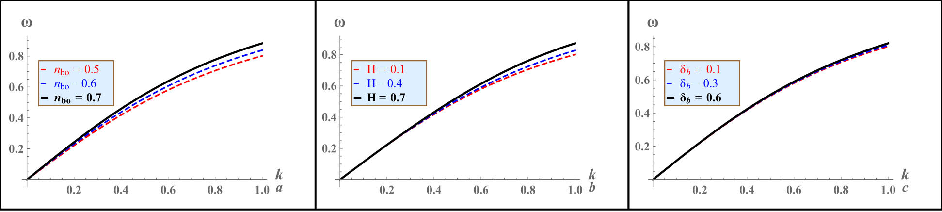
The wave frequency
The reduced equations for
The compatibility condition obtained from the above-reduced equations is
In Eq. (14),

The wave packets group velocity
The reduced equations of second-order,
The coefficients
The second-order zero harmonic quantities obtained from reduced equations for
Finally, we obtain the following cubic NLSE by substituting the above derived expressions into the
Eq. (18) is referred to as NLSE, with
and
The coefficient

The coefficient
The nonlinearity coefficient

The coefficient
4 MI analysis
We now provide a quick overview of the NLSE (18) stability analysis by linearizing around the monochromatic (Stokes’) wave solution [92,93] of the form
The stability/instability of plane-wave solutions under external perturbations can be inferred from the signs of
Before we proceed to envelope solitons formation, we should first identify parametric stable and unstable regions based on the sign of

The ratio
5 Envelope soliton formation
In this study, we examined IAWs in quantum plasma with an ion beam. Model quantum plasma is considered for the numerical analysis by choosing the values for ion beam density
The nonlinear excitations in the form of bright and dark envelope solitons are described by the localized solution of the NLSE (18). By using
The bright soliton solution of NLSE (18) is associated with a positive sign of
where

Bright envelope soliton solution (23) is plotted in unstable region (i.e.,
Dark envelope soliton solution of NLSE (18) is associated with a negative sign of
These excitations can appear as black solitons (vanishing potential at

Dark (black) envelope soliton solution (24) is plotted in stable region (i.e.,

Dark (gray) envelope soliton solution (24) is plotted in stable region (i.e.,
6 Summary
In this article, we have studied the low-frequency IAWs in unmagnetized quantum plasma including the effects of ion beams. One of the reductive perturbation methods, i.e., DEM has been used for reducing the basic plasma model equations to the cubic NLSE. The nonlinearity and dispersion coefficients of the NLSE have been explicitly expressed, and their parametric dependency on the relevant plasma parameters has been investigated. The MI and growth rate of envelope excitations have been estimated based on the coefficients of the NLSE. We noted that the critical wavenumber
For clarity and precision, it is important to highlight that we have utilized a QHD model, which incorporates two key quantum effects, i.e., Bohm potential and and quantum statistical terms. Our model is valid for small values of
7 Future work
The phenomena of RWs and breathers are among the most enigmatic occurrences, producing many consequences that can significantly influence the features of the system under investigation. Consequently, future research may investigate the characteristics of nonplanar RWs and breathers [98–101], dissipative RWs and breathers [102,103], as well as the methods for regulating their manifestation in the system under examination, depending on the necessity for their presence or avoidance.
Acknowledgments
The authors aknowledge the financial support provided by Princess Nourah bint Abdulrahman University Researchers Supporting Project number (PNURSP2025R439), Princess Nourah bint Abdulrahman University, Riyadh, Saudi Arabia. The support of Prince sattam bin Abdulaziz University project number (PSAU/2025/R/1446) is also acknowledged.
-
Funding information: The authors are thankful for the financial support provided by Princess Nourah bint Abdulrahman University Researchers Supporting Project number (PNURSP2025R439), Princess Nourah bint Abdulrahman University, Riyadh, Saudi Arabia. The support of Prince sattam bin Abdulaziz University project number (PSAU/2025/R/1446) is also acknowledged.
-
Author contributions: Fazal Wahed: formal analysis, investigation, writing – original draft. Ata-ur-Rahman: methodology, writing – review and editing. S. Neelam Naeem: investigation, writing – original draft. R. A. Alharbey: investigation, methodology. Maryam Al Huwayz: formal analysis, writing – original draft. Lamiaa S. El-Sherif: investigation, writing – review and editing. Samir A. El-Tantawy: formal analysis, investigation, methodology, supervision, writing – review and editing. All authors have accepted responsibility for the entire content of this manuscript and approved its submission.
-
Conflict of interest: The authors state no conflict of interest.
-
Data availability statement: All data generated or analysed during this study are included in this published article.
Appendix
The expressions for the coefficients of Eqs (15), (16), and (17) are:
References
[1] Killian TC. Ultracold neutral plasmas. Sci. 2007;316:705–8. 10.1126/science.1130556Search in Google Scholar PubMed
[2] Marklund M, Shukla PK. Nonlinear collective effects in photon-photon and photon-plasma interactions. Rev M Phy. 2006;78:591. 10.1103/RevModPhys.78.591Search in Google Scholar
[3] Becker K, Koutsospyros A, Yin SM, Christodoulatos C, Abramzon N, Joaquin JC, et al. Environmental and biological applications of microplasmas. Plasma Phys Contrl Fus. 2005;47:513. 10.1088/0741-3335/47/12B/S37Search in Google Scholar
[4] Markowich PA, Ringhofer CA, Schmeiser C. The drift diffusion equations. Semiconductor equations. New York: Springer-Verlag; 1990. p. 104–74. 10.1007/978-3-7091-6961-2_4Search in Google Scholar
[5] Jung YD. Quantum-mechanical effects on electron-electron scattering in dense high-temperature plasmas. Phys Plasmas. 2001;8(8):3842–4. 10.1063/1.1386430Search in Google Scholar
[6] Hossen MA, Hossen MR, Mamun AA. Modified ion-acoustic shock waves and double layers in a degenerate electron-positron-ion plasma in presence of heavy negative ions. Braz J Phys. 2014;44:703–10. 10.1007/s13538-014-0267-xSearch in Google Scholar
[7] Manfredi G. Proceedings of the Workshop on kinetic theory. Fields Inst Commun. 2005;46:263. 10.1090/fic/046/10Search in Google Scholar
[8] Qamar A, Rahman A, Mirza AM. Tripolar vortex formation in dense quantum plasma with ion-temperature gradients. Phys Plasmas. 2012;19:052303. 10.1063/1.4714648Search in Google Scholar
[9] Hass F. Quantum plasmas. An hydrodynamic approach. New York, NY, USA: Springer; 2011. 10.1007/978-1-4419-8201-8Search in Google Scholar
[10] Madelung E. Quantum theory in hydrodynamic form. Z Phys. 1927;40:322–36. 10.1007/BF01400372Search in Google Scholar
[11] Manfredi G, Haas F. Self-consistent fluid model for a quantum electron gas. Phys Rev B. 2001;64:075316. 10.1103/PhysRevB.64.075316Search in Google Scholar
[12] Gardner CL. The quantum hydrodynamic model for semiconductor devices. SIAM J Appl Maths. 1994;54:409–27. 10.1137/S0036139992240425Search in Google Scholar
[13] Gardner CL. Numerical simulation of a steady-state electron shock wave in a submicrometer semiconductor device. IEEE Trans Electron Devices. 1991;38:392–8. 10.1109/16.69922Search in Google Scholar
[14] Haas H, Garcia LG, Goedert J. Quantum ion-acoustic waves. Phys Plasmas. 2003;10:3858. 10.1063/1.1609446Search in Google Scholar
[15] Mushtaq A, Khan SA. Ion acoustic solitary wave with weakly transverse perturbations in quantum electron-positron-ion plasma. Phys Plasmas. 2007;14:052307. 10.1063/1.2727474Search in Google Scholar
[16] Rajabi B, Mohammadnejad M. Modulational instability of ion-acoustic waves in a dense quantum plasma. Phys Plasmas. 2023;8:30. 10.1063/5.0154769Search in Google Scholar
[17] Chandra S, Paul SN, Ghosh B. Linear and non-linear propagation of electron plasma waves in quantum plasma. Indian J Pure Appl Phys. 2012;50:314–9. Search in Google Scholar
[18] Celata CM, Bieniosek FM, Henestroza E, Kwan JW, Lee EP, Logan G, et al. Progress in heavy ion fusion research. Phys Plasmas. 2003;10:2064–70. 10.1063/1.1560611Search in Google Scholar
[19] Sharp WM, Callahan DA, Tabak M, Yu SS, Peterson PF, Welch DR, et al. Modeling chamber transport for heavy-ion fusion. Fusion Sci Tech. 2003;43:393–400. 10.13182/FST03-A283Search in Google Scholar
[20] Davidson RC, Logan BG, Barnard JJ, Bieniosek FM, Briggs RJ, Callahan DA, et al. US heavy ion beam research for high energy density physics applications and fusion. In J de Phys IV (Proceedings) EDP Sci. 2006;133:731–41. 10.2172/878296Search in Google Scholar
[21] Colak S, Fitzpatrick BJ, Bhargava RN. Electron beam pumped II–VI lasers. J Cryst Growth. 1985;72:504. 10.1016/0022-0248(85)90198-8Search in Google Scholar
[22] Gurskii AL, Lutsenko EV, Mitcovets AI, Yablonskii GP. High-efficiency electron-beam-pumped semiconductor laser emitters. Phys B. 1993;185:505. 10.1016/B978-0-444-81573-6.50082-7Search in Google Scholar
[23] Liu L, Jia L, Liang Z, Sankai S, Xifeng R. Polarization independent tunable near-perfect absorber based on graphene-BaO arrays and Ag-dielectric Bragg reflector composite structure. Diamond Relat Mater. 2025;152:111958. 10.1016/j.diamond.2025.111958Search in Google Scholar
[24] Richa, Bhupendra KS, Bandar A, David L. Intelligent neuro-computational modelling for MHD nanofluid flow through a curved stretching sheet with entropy optimization: Koo–Kleinstreuer–Li approach. J Comput Des Eng. 2024;11:164–83. 10.1093/jcde/qwae078Search in Google Scholar
[25] Sorensen AH, Bonderup E. Electron cooling. Nucl Instrum Methods Phys Res. 1983;215:27. 10.1016/0167-5087(83)91288-7Search in Google Scholar
[26] Goldman SR, Hofmann I. Electron cooling of high-Z ion beams parallel to a guide magnetic field. IEEE Trans Plasma Sci. 1990;18:789. 10.1109/27.62344Search in Google Scholar
[27] Kumar A, Sharma BK, Almohsen B, Pérez LM, Urbanowicz K. Artificial neural network analysis of Jeffrey hybrid nanofluid with gyrotactic microorganisms for optimizing solar thermal collector efficiency. Sci Rep. 2025;15(1):4729. 10.1038/s41598-025-88877-6Search in Google Scholar PubMed PubMed Central
[28] Shilei X, Nan Y, Haoyu G, Guangyuan S, Ming L, Yoshihiro D, et al. Combination of plasma acoustic emission signal and laser-induced breakdown spectroscopy for accurate classification of steel. Anal Chim Acta. 2025;1336:343496. 10.1016/j.aca.2024.343496Search in Google Scholar PubMed
[29] Anup K, Bhupendra KS, Madhu S, Bandar A, Ioannis ES. Entropy generation optimization for casson hybrid nanofluid flow along a curved surface with bioconvection mechanism and exothermic/endothermic catalytic reaction. Adv Theor Simul. 2025;8:2401554. 10.1002/adts.202401554Search in Google Scholar
[30] Krushelnick K, Clark EL, Allott R, Beg FN, Danson CN, Machacek A, et al. Ultrahigh-intensity laser-produced plasmas as a compact heavy ion injection source. IEEE Trans Plasma Sci. 2000;28:1184. 10.1109/27.893296Search in Google Scholar
[31] Kaganovich ID, Startsev EA, Sefkow AB, Davidson RC. Charge and current neutralization of an ion-beam pulse propagating in a background plasma along a solenoidal magnetic field. Phys Rev Lett. 2007;99:235002. 10.1103/PhysRevLett.99.235002Search in Google Scholar PubMed
[32] Renk TJ, Mann GA, Torres GA. Performance of a pulsed ion beam with a renewable cryogenically cooled ion source. Laser Particle Beams. 2008;26:545. 10.1017/S026303460800058XSearch in Google Scholar
[33] Goldman MV. Progress and problems in the theory of type III solar radio emission. Solar Phys. 1983;89:403–42. 10.1007/BF00217259Search in Google Scholar
[34] Hoffmann RA, Evans DS. Field-aligned electron bursts at high latitudes observed by Ogo 4. J Geophys Res. 1968;73:6201–14. 10.1029/JA073i019p06201Search in Google Scholar
[35] Alotaibi MA, El-Sapa S. Effect of permeability on the interaction between two spheres translating through a couple stress fluid. Fluid Dyn Res. 2025; 57(1):015503. 10.1088/1873-7005/ada855Search in Google Scholar
[36] Al-Hanaya A, El-Sapa S. Impact of permeability and fluid parameters in couple stress media on rotating eccentric spheres. Open Phys. 2024;22(1):20240112. 10.1515/phys-2024-0112Search in Google Scholar
[37] El-Sapa S, Alotaibi MA. Migration of two rigid spheres translating within an infinite couple stress fluid under the impact of magnetic field. Open Phys. 2024;22(1):20240085. 10.1515/phys-2024-0085Search in Google Scholar
[38] Krivoruchko SM, Fainberg VB, Shapiro VD, Shevchenko VI. Solitary charge density waves in a magnetoactive plasma. Sov JETP. 1975;40:1039–43. Search in Google Scholar
[39] Deka MK, Adhikary NC, Misra AP, Bailung H, Nakamura Y. Characteristics of ion-acoustic solitary wave in a laboratory dusty plasma under the influence of ion-beam. Phys Plasmas. 2012;19:103704. 10.1063/1.4757217Search in Google Scholar
[40] Chatterjee P, Roychoudhury R. The effect of finite ion temperature on solitary waves in a plasma with an ion beam. Phys Plasmas. 1995;2:1352. 10.1063/1.871347Search in Google Scholar
[41] Abrol PS, Tagare SG. Ion-acoustic solitary waves in an ion-beam–plasma system with nonisothermal electrons. Phys Lett A. 1979;75:74–6. 10.1016/0375-9601(79)90281-0Search in Google Scholar
[42] Gell Y, Roth I. The effects of an ion beam on the motion of solitons in an ion beam–plasma system. Plasma Phys. 1977;19:915. 10.1088/0032-1028/19/10/002Search in Google Scholar
[43] Das R, Deka P. Korteweg-de Vries solutions in high relativistic electron beam plasma. Int J Eng Res. 2015;6:864–70. Search in Google Scholar
[44] Misra AP, Adhikary NC. Large amplitude solitary waves in ion-beam plasmas with charged dust impurities. Phys Plasmas. 2011;18:122112. 10.1063/1.3671951Search in Google Scholar
[45] Huibin L, Kelin W. Solitons in an ion-beam plasma. J Plasma Phys. 1990;44(1):151–65. 10.1017/S0022377800015075Search in Google Scholar
[46] Zank GP, McKenzie JF. Solitons in an ion-beam plasma. J Plasma Phys. 1998;39:183–91. 10.1017/S0022377800012976Search in Google Scholar
[47] Karmakar B, Das GC, Singh I. Ion-acoustic solitary waves in ion-beam plasma with multiple-electron-temperatures. Plasma Phys Contr Fus. 1988;30:1167. 10.1088/0741-3335/30/9/006Search in Google Scholar
[48] Kaur N, Singh K, Saini NS. Effect of ion beam on the characteristics of ion acoustic Gardner solitons and double layers in a multicomponent superthermal plasma. Phys Plasmas. 2017;24:092108. 10.1063/1.5000051Search in Google Scholar
[49] Kaur N, Singh K, Ghai Y, Saini NS. Dust acoustic shock waves in magnetized dusty plasma. Plasma Sci Tech. 2018;20:074009. 10.1088/2058-6272/aac37aSearch in Google Scholar
[50] Kourakis I, Shukla PK. Oblique amplitude modulation of dust-acoustic plasma waves. Phys Scr. 2004;69:316. 10.1238/Physica.Regular.069a00316Search in Google Scholar
[51] Taniuti T, N. Yajima N. Perturbation method for a nonlinear wave modulation III. J Math Phys. 1969;10:1369. 10.1063/1.1664975Search in Google Scholar
[52] Albalawi W, El-Tantawy SA, Salas AH. On the rogue wave solution in the framework of a Korteweg-de Vries equation. Results Phys. 2021;30:104847. 10.1016/j.rinp.2021.104847Search in Google Scholar
[53] Hashmi T, Jahangir R, Masood W, Alotaibi BM, Ismaeel SME, El-Tantawy SA. Head-on collision of ion-acoustic (modified) Korteweg-de Vries solitons in Saturn’s magnetosphere plasmas with two temperature superthermal electrons. Phys Fluids. 2023;35:103104. 10.1063/5.0171220Search in Google Scholar
[54] El-Tantawy SA. Nonlinear dynamics of soliton collisions in electronegative plasmas: The phase shifts of the planar KdV-and mkdV-soliton collisions. Chaos Solitons Fractals. 2016;93:162. 10.1016/j.chaos.2016.10.011Search in Google Scholar
[55] Wazwaz A-M, Alhejaili W, El-Tantawy SA, Study on extensions of (modified) Korteweg-de Vries equations: Painlevé integrability and multiple soliton solutions in fluid mediums. Physics of Fluids. 2023;35:093110. 10.1063/5.0169733Search in Google Scholar
[56] Kashkari BS, El-Tantawy SA, Salas AH, El-Sherif LS. Homotopy perturbation method for studying dissipative nonplanar solitons in an electronegative complex plasma. Chaos Solitons Fractals. 2020;130:109457. 10.1016/j.chaos.2019.109457Search in Google Scholar
[57] El-Tantawy SA, Wazwaz A-M. Anatomy of modified Korteweg-de Vries equation for studying the modulated envelope structures in non-Maxwellian dusty plasmas: Freak waves and dark soliton collisions. Phys Plasmas. 2018;25:092105. 10.1063/1.5045247Search in Google Scholar
[58] Albalawi W, El-Tantawy SA, SAlkhateebadah SA. The phase shift analysis of the colliding dissipative KdV solitons. J Ocean Eng Sci. 2022;7:521. 10.1016/j.joes.2021.09.021Search in Google Scholar
[59] Gill TS, Bains AS, Saini NS, Bedi C. Ion-acoustic envelope excitations in electron-positron-ion plasma with nonthermal electrons. Phys Lett A. 2010;374:3210–5. 10.1016/j.physleta.2010.05.046Search in Google Scholar
[60] El-Tantawy SA, Wazwaz A-M, Schlickeiser R. Solitons collision and freak waves in a plasma with Cairns-Tsallis particle distributions, Plasma Phys Control Fusion. 2015;57:125012. 10.1088/0741-3335/57/12/125012Search in Google Scholar
[61] Ali Shan S, El-Tantawy SA. The impact of positrons beam on the propagation of super freak waves in electron-positron-ion plasmas. Phys Plasmas. 2016;23:072112. 10.1063/1.4958315Search in Google Scholar
[62] Esfandyari-Kalejahi A, Kourakis I, Dasmalchi B, Sayarizadeh M. Nonlinear propagation of modulated ion-acoustic plasma waves in the presence of an electron beam. Phys Plasmas. 2006;13:4. 10.1063/1.2182928Search in Google Scholar
[63] Kourakis I, Shukla PK. Ion-acoustic waves in a two-electron-temperature plasma: oblique modulation and envelope excitations. J Phys A Math Gen. 2003;36:11901. 10.1088/0305-4470/36/47/015Search in Google Scholar
[64] Kourakis I, Shukla PK. Exact theory for localized envelope modulated electrostatic wavepackets in space and dusty plasmas. Non Pro Geophys. 2005;12:407. 10.5194/npg-12-407-2005Search in Google Scholar
[65] Esfandyari-Kalejahi A, Asgari H. Ion-acoustic solitary excitations in a two-electron-temperature plasma with adiabatic warm ions. Phys Plasmas. 2005;12:102302. 10.1063/1.2072867Search in Google Scholar
[66] Krall NA, Trivelpiece AW. Fundamentals of plasma physics and principles of plasma physics. NewYork: McGraw-Hill; 1973. 10.1119/1.1987587Search in Google Scholar
[67] Stix T. Waves in plasmas. New York: American Institute of Physics; 1992. Search in Google Scholar
[68] Rahman A. Electrostatic Rogue waves in a degenerate Thomas-Fermi plasma. Braz J Phys. 2019;49:517–25. 10.1007/s13538-019-00676-3Search in Google Scholar
[69] Irshad M, Khalid M. Modulational instability of ion acoustic excitations in a plasma with a kappa-deformed Kaniadakis electron distribution. Eur Phys J Plus. 2022;137:893. 10.1140/epjp/s13360-022-03098-4Search in Google Scholar
[70] Kivshar Yu S, Peyrard M. Modulational instabilities in discrete lattices. Phys Rev A. 1992;46:3198. 10.1103/PhysRevA.46.3198Search in Google Scholar
[71] Remoissenet M. Waves called solitons. Berlin: Springer; 1994. 10.1007/978-3-662-03057-8Search in Google Scholar
[72] Hasegawa A. Plasma instabilities and nonlinear effects. Berlin: Springer; 1975. 10.1007/978-3-642-65980-5Search in Google Scholar
[73] Shukla PK, Stenflo L, Fedele R. Modulational instability of two colliding Bose–Einstein condensates. Phys Scr. 2001;64:553. 10.1238/Physica.Regular.064a00553Search in Google Scholar
[74] Theocharis G, Rapti Z, Kevrekidis PG, Frantzeskakis DJ, Konotop VV. Modulational instability of Gross-Pitaevskii-type equations in 1 + 1 dimensions. Phys Rev A. 2003; 67:063610. 10.1103/PhysRevA.67.063610Search in Google Scholar
[75] Davydov AS. Solitons in molecular systems. Dordrecht: Kluwer; 1985. 10.1007/978-94-017-3025-9Search in Google Scholar
[76] Bilbault JM, Marquie P, Michaux B. Modulational instability of two counterpropagating waves in an experimental transmission line. Phys Rev E. 1995;51:817. 10.1103/PhysRevE.51.817Search in Google Scholar PubMed
[77] Agrawal G. Fiber optic communication systems. New York: Wiley; 2002. 10.1002/0471221147Search in Google Scholar
[78] Watanabe S. Self-modulation of a nonlinear ionwave packet. J Plasma Phys. 1977;17:487. 10.1017/S0022377800020754Search in Google Scholar
[79] Irshad M, Khalid M, Khan S, Alotaibi BM, El-Sherif LS, El-Tantawy SA. Effect of kappa-deformed Kaniadakis distribution on the modulational instability of electron-acoustic waves in a non-Maxwellian plasma. Phys Fluids. 2023:35:105116. 10.1063/5.0171327Search in Google Scholar
[80] Wahed F, Rahman AU, Alyousef HA, El-Sherif LS, El-Tantawy SA. Modulational instability and associated low-frequency dust-acoustic waves in a degenerate Thomas-Fermiplasma: Envelope solitons and rogue waves. J Low Freq Noise Vibr Act Control. 2024;16:14613484241308433. 10.1177/14613484241308433Search in Google Scholar
[81] El-Tantawy SA. Ion-acoustic waves in ultracold neutral plasmas: modulational instability and dissipative rogue waves. Phys Lett. 2017;381:787–91. 10.1016/j.physleta.2016.12.052Search in Google Scholar
[82] Kourakis I, Shukla PK. Electron-acoustic plasma waves: oblique modulation and envelope solitons. Phy Rew E. 2004;69(3):036411. 10.1103/PhysRevE.69.036411Search in Google Scholar PubMed
[83] Paul I, Chatterjee A, Paul SN. Nonlinear propagation of ion acoustic waves in quantum plasma in the presence of an ion beam. Laser Part Beams. 2019;37:370–80. 10.1017/S0263034619000697Search in Google Scholar
[84] Az-Zo’bi Emad A. On the reduced differential transform method and its application to the generalized Burgers-Huxley equation. App Math Sci. 2014;8(177):8823–31. 10.12988/ams.2014.410835Search in Google Scholar
[85] Az-Zo’bi Emad A. Peakon and solitary wave solutions for the modified Fornberg-Whitham equation using simplest equation method. Int J Math Comput Sci. 2019;14(3):635–45. Search in Google Scholar
[86] Asano N, Taniuti T, Yajima N. Perturbation method for a nonlinear wave modulation. II. J Math Phys. 1969;10:2020. 10.1063/1.1664797Search in Google Scholar
[87] Hasegawa A. Stimulated modulational instabilities of plasma waves. Phys Rev A. 1970;1:1746. 10.1103/PhysRevA.1.1746Search in Google Scholar
[88] Hasegawa A. Theory and computer experiment on self-trapping instability of plasma cyclotron waves. Phys Fluids. 1972;15(5):870–81. 10.1063/1.1693996Search in Google Scholar
[89] Debnath L. Nonlinear partial differential equations for scientists and engineers. Birkauser Boston; 2005. 10.1007/b138648Search in Google Scholar
[90] Taniuti T. Reductive perturbation method and far fields of wave equations. Supp Prog Theor Phys. 1974;55:1. 10.1143/PTPS.55.1Search in Google Scholar
[91] Gardner CS, Morikawa GK. The effect of temperature on the width of a small-amplitude, solitary wave in a collision-free plasma. Comm Pur App Math XVIII. 1965;18:35–49. 10.1002/cpa.3160180107Search in Google Scholar
[92] Remoissenet R. Waves called solitons. Berlin: Springer; 1996. 10.1007/978-3-662-03321-0Search in Google Scholar
[93] Fedele R, Schamel H. Solitary waves in the Madelung’s fluid: Connection between the nonlinear Schrödinger equation and the Korteweg-de Vries equation. Eur Phys J B. 2002;27:313. 10.1140/epjb/e2002-00160-7Search in Google Scholar
[94] Dauxois T, Peyrard M. Physics of solitons. Cambridge: Cambridge University Press; 2006. Search in Google Scholar
[95] Misra AP, Ghosh NK. Modulational instability of ion-acoustic wave packets in quantum pair-ion plasmas. Astrophys Space Sci. 2011;331:605–9. 10.1007/s10509-010-0472-1Search in Google Scholar
[96] Garcia LG, Haas F, De Oliveira LPL, Goedert J. Modified Zakharov equations for plasmas with a quantum correction. Phys Plasmas. 2005;12(1):012302. 10.1063/1.1819935Search in Google Scholar
[97] Yu Z, Lü X. Data-driven solutions and parameter discovery of the extended higher-order nonlinear Schrödinger equation in optical fibers. Phys D. 2024;468:134284. 10.1016/j.physd.2024.134284Search in Google Scholar
[98] El-Tantawy SA, Aboelenen T. Simulation study of planar and nonplanar super rogue waves in an electronegative plasma: Local discontinuous Galerkin method. Phys Plasmas. 2017;24:052118. 10.1063/1.4983327Search in Google Scholar
[99] El-Tantawy SA, AlharbeyRA, Salas AH. Novel approximate analytical and numerical cylindrical rogue wave and breathers solutions: An application to electronegative plasma. Chaos Solitons Fractals. 2022;155:111776. 10.1016/j.chaos.2021.111776Search in Google Scholar
[100] El-Tantawy SA, Salas AH, Alyousef HA, Alharthi MR. Novel approximations to a nonplanar nonlinear Schrödinger equation and modeling nonplanar rogue waves/breathers in a complexplasma. Chaos Solitons Fractals. 2022;1635:112612. 10.1016/j.chaos.2022.112612Search in Google Scholar
[101] El-Tantawy SA, El-Awady EI. Cylindrical and spherical Akhmediev breather and freak waves in ultracold neutral plasmas. Phys Plasmas. 2018;25:012121. 10.1063/1.4989652Search in Google Scholar
[102] Aljahdaly NH, El-Tantawy SA, Wazwaz A-M, Ashi HA. Adomian decomposition method for modelling the dissipative higher-order rogue waves in a superthermal collisional plasma. J Taibah Univ Sci. 2021;15:971. 10.1080/16583655.2021.2012373Search in Google Scholar
[103] El-Tantawy SA, Salas AH, Alharthi MR. On the analytical and numerical solutions of the linear damped NLSE for modeling dissipative freak waves and breathers in nonlinear and dispersive mediums: an application to a pair-ion plasma. Front Phys. 2021;9:580224. 10.3389/fphy.2021.580224Search in Google Scholar
© 2025 the author(s), published by De Gruyter
This work is licensed under the Creative Commons Attribution 4.0 International License.
Articles in the same Issue
- Research Articles
- Single-step fabrication of Ag2S/poly-2-mercaptoaniline nanoribbon photocathodes for green hydrogen generation from artificial and natural red-sea water
- Abundant new interaction solutions and nonlinear dynamics for the (3+1)-dimensional Hirota–Satsuma–Ito-like equation
- A novel gold and SiO2 material based planar 5-element high HPBW end-fire antenna array for 300 GHz applications
- Explicit exact solutions and bifurcation analysis for the mZK equation with truncated M-fractional derivatives utilizing two reliable methods
- Optical and laser damage resistance: Role of periodic cylindrical surfaces
- Numerical study of flow and heat transfer in the air-side metal foam partially filled channels of panel-type radiator under forced convection
- Water-based hybrid nanofluid flow containing CNT nanoparticles over an extending surface with velocity slips, thermal convective, and zero-mass flux conditions
- Dynamical wave structures for some diffusion--reaction equations with quadratic and quartic nonlinearities
- Solving an isotropic grey matter tumour model via a heat transfer equation
- Study on the penetration protection of a fiber-reinforced composite structure with CNTs/GFP clip STF/3DKevlar
- Influence of Hall current and acoustic pressure on nanostructured DPL thermoelastic plates under ramp heating in a double-temperature model
- Applications of the Belousov–Zhabotinsky reaction–diffusion system: Analytical and numerical approaches
- AC electroosmotic flow of Maxwell fluid in a pH-regulated parallel-plate silica nanochannel
- Interpreting optical effects with relativistic transformations adopting one-way synchronization to conserve simultaneity and space–time continuity
- Modeling and analysis of quantum communication channel in airborne platforms with boundary layer effects
- Theoretical and numerical investigation of a memristor system with a piecewise memductance under fractal–fractional derivatives
- Tuning the structure and electro-optical properties of α-Cr2O3 films by heat treatment/La doping for optoelectronic applications
- High-speed multi-spectral explosion temperature measurement using golden-section accelerated Pearson correlation algorithm
- Dynamic behavior and modulation instability of the generalized coupled fractional nonlinear Helmholtz equation with cubic–quintic term
- Study on the duration of laser-induced air plasma flash near thin film surface
- Exploring the dynamics of fractional-order nonlinear dispersive wave system through homotopy technique
- The mechanism of carbon monoxide fluorescence inside a femtosecond laser-induced plasma
- Numerical solution of a nonconstant coefficient advection diffusion equation in an irregular domain and analyses of numerical dispersion and dissipation
- Numerical examination of the chemically reactive MHD flow of hybrid nanofluids over a two-dimensional stretching surface with the Cattaneo–Christov model and slip conditions
- Impacts of sinusoidal heat flux and embraced heated rectangular cavity on natural convection within a square enclosure partially filled with porous medium and Casson-hybrid nanofluid
- Stability analysis of unsteady ternary nanofluid flow past a stretching/shrinking wedge
- Solitonic wave solutions of a Hamiltonian nonlinear atom chain model through the Hirota bilinear transformation method
- Bilinear form and soltion solutions for (3+1)-dimensional negative-order KdV-CBS equation
- Solitary chirp pulses and soliton control for variable coefficients cubic–quintic nonlinear Schrödinger equation in nonuniform management system
- Influence of decaying heat source and temperature-dependent thermal conductivity on photo-hydro-elasto semiconductor media
- Dissipative disorder optimization in the radiative thin film flow of partially ionized non-Newtonian hybrid nanofluid with second-order slip condition
- Bifurcation, chaotic behavior, and traveling wave solutions for the fractional (4+1)-dimensional Davey–Stewartson–Kadomtsev–Petviashvili model
- New investigation on soliton solutions of two nonlinear PDEs in mathematical physics with a dynamical property: Bifurcation analysis
- Mathematical analysis of nanoparticle type and volume fraction on heat transfer efficiency of nanofluids
- Creation of single-wing Lorenz-like attractors via a ten-ninths-degree term
- Optical soliton solutions, bifurcation analysis, chaotic behaviors of nonlinear Schrödinger equation and modulation instability in optical fiber
- Chaotic dynamics and some solutions for the (n + 1)-dimensional modified Zakharov–Kuznetsov equation in plasma physics
- Fractal formation and chaotic soliton phenomena in nonlinear conformable Heisenberg ferromagnetic spin chain equation
- Single-step fabrication of Mn(iv) oxide-Mn(ii) sulfide/poly-2-mercaptoaniline porous network nanocomposite for pseudo-supercapacitors and charge storage
- Novel constructed dynamical analytical solutions and conserved quantities of the new (2+1)-dimensional KdV model describing acoustic wave propagation
- Tavis–Cummings model in the presence of a deformed field and time-dependent coupling
- Spinning dynamics of stress-dependent viscosity of generalized Cross-nonlinear materials affected by gravitationally swirling disk
- Design and prediction of high optical density photovoltaic polymers using machine learning-DFT studies
- Robust control and preservation of quantum steering, nonlocality, and coherence in open atomic systems
- Coating thickness and process efficiency of reverse roll coating using a magnetized hybrid nanomaterial flow
- Dynamic analysis, circuit realization, and its synchronization of a new chaotic hyperjerk system
- Decoherence of steerability and coherence dynamics induced by nonlinear qubit–cavity interactions
- Finite element analysis of turbulent thermal enhancement in grooved channels with flat- and plus-shaped fins
- Modulational instability and associated ion-acoustic modulated envelope solitons in a quantum plasma having ion beams
- Statistical inference of constant-stress partially accelerated life tests under type II generalized hybrid censored data from Burr III distribution
- On solutions of the Dirac equation for 1D hydrogenic atoms or ions
- Entropy optimization for chemically reactive magnetized unsteady thin film hybrid nanofluid flow on inclined surface subject to nonlinear mixed convection and variable temperature
- Stability analysis, circuit simulation, and color image encryption of a novel four-dimensional hyperchaotic model with hidden and self-excited attractors
- A high-accuracy exponential time integration scheme for the Darcy–Forchheimer Williamson fluid flow with temperature-dependent conductivity
- Novel analysis of fractional regularized long-wave equation in plasma dynamics
- Development of a photoelectrode based on a bismuth(iii) oxyiodide/intercalated iodide-poly(1H-pyrrole) rough spherical nanocomposite for green hydrogen generation
- Investigation of solar radiation effects on the energy performance of the (Al2O3–CuO–Cu)/H2O ternary nanofluidic system through a convectively heated cylinder
- Quantum resources for a system of two atoms interacting with a deformed field in the presence of intensity-dependent coupling
- Studying bifurcations and chaotic dynamics in the generalized hyperelastic-rod wave equation through Hamiltonian mechanics
- A new numerical technique for the solution of time-fractional nonlinear Klein–Gordon equation involving Atangana–Baleanu derivative using cubic B-spline functions
- Interaction solutions of high-order breathers and lumps for a (3+1)-dimensional conformable fractional potential-YTSF-like model
- Hydraulic fracturing radioactive source tracing technology based on hydraulic fracturing tracing mechanics model
- Numerical solution and stability analysis of non-Newtonian hybrid nanofluid flow subject to exponential heat source/sink over a Riga sheet
- Numerical investigation of mixed convection and viscous dissipation in couple stress nanofluid flow: A merged Adomian decomposition method and Mohand transform
- Effectual quintic B-spline functions for solving the time fractional coupled Boussinesq–Burgers equation arising in shallow water waves
- Analysis of MHD hybrid nanofluid flow over cone and wedge with exponential and thermal heat source and activation energy
- Solitons and travelling waves structure for M-fractional Kairat-II equation using three explicit methods
- Impact of nanoparticle shapes on the heat transfer properties of Cu and CuO nanofluids flowing over a stretching surface with slip effects: A computational study
- Computational simulation of heat transfer and nanofluid flow for two-sided lid-driven square cavity under the influence of magnetic field
- Irreversibility analysis of a bioconvective two-phase nanofluid in a Maxwell (non-Newtonian) flow induced by a rotating disk with thermal radiation
- Hydrodynamic and sensitivity analysis of a polymeric calendering process for non-Newtonian fluids with temperature-dependent viscosity
- Exploring the peakon solitons molecules and solitary wave structure to the nonlinear damped Kortewege–de Vries equation through efficient technique
- Modeling and heat transfer analysis of magnetized hybrid micropolar blood-based nanofluid flow in Darcy–Forchheimer porous stenosis narrow arteries
- Activation energy and cross-diffusion effects on 3D rotating nanofluid flow in a Darcy–Forchheimer porous medium with radiation and convective heating
- Insights into chemical reactions occurring in generalized nanomaterials due to spinning surface with melting constraints
- Influence of a magnetic field on double-porosity photo-thermoelastic materials under Lord–Shulman theory
- Soliton-like solutions for a nonlinear doubly dispersive equation in an elastic Murnaghan's rod via Hirota's bilinear method
- Analytical and numerical investigation of exact wave patterns and chaotic dynamics in the extended improved Boussinesq equation
- Nonclassical correlation dynamics of Heisenberg XYZ states with (x, y)-spin--orbit interaction, x-magnetic field, and intrinsic decoherence effects
- Exact traveling wave and soliton solutions for chemotaxis model and (3+1)-dimensional Boiti–Leon–Manna–Pempinelli equation
- Unveiling the transformative role of samarium in ZnO: Exploring structural and optical modifications for advanced functional applications
- On the derivation of solitary wave solutions for the time-fractional Rosenau equation through two analytical techniques
- Analyzing the role of length and radius of MWCNTs in a nanofluid flow influenced by variable thermal conductivity and viscosity considering Marangoni convection
- Advanced mathematical analysis of heat and mass transfer in oscillatory micropolar bio-nanofluid flows via peristaltic waves and electroosmotic effects
- Exact bound state solutions of the radial Schrödinger equation for the Coulomb potential by conformable Nikiforov–Uvarov approach
- Some anisotropic and perfect fluid plane symmetric solutions of Einstein's field equations using killing symmetries
- Nonlinear dynamics of the dissipative ion-acoustic solitary waves in anisotropic rotating magnetoplasmas
- Curves in multiplicative equiaffine plane
- Exact solution of the three-dimensional (3D) Z2 lattice gauge theory
- Propagation properties of Airyprime pulses in relaxing nonlinear media
- Symbolic computation: Analytical solutions and dynamics of a shallow water wave equation in coastal engineering
- Wave propagation in nonlocal piezo-photo-hygrothermoelastic semiconductors subjected to heat and moisture flux
- Comparative reaction dynamics in rotating nanofluid systems: Quartic and cubic kinetics under MHD influence
- Laplace transform technique and probabilistic analysis-based hypothesis testing in medical and engineering applications
- Physical properties of ternary chloro-perovskites KTCl3 (T = Ge, Al) for optoelectronic applications
- Gravitational length stretching: Curvature-induced modulation of quantum probability densities
- The search for the cosmological cold dark matter axion – A new refined narrow mass window and detection scheme
- A comparative study of quantum resources in bipartite Lipkin–Meshkov–Glick model under DM interaction and Zeeman splitting
- PbO-doped K2O–BaO–Al2O3–B2O3–TeO2-glasses: Mechanical and shielding efficacy
- Nanospherical arsenic(iii) oxoiodide/iodide-intercalated poly(N-methylpyrrole) composite synthesis for broad-spectrum optical detection
- Sine power Burr X distribution with estimation and applications in physics and other fields
- Numerical modeling of enhanced reactive oxygen plasma in pulsed laser deposition of metal oxide thin films
- Dynamical analyses and dispersive soliton solutions to the nonlinear fractional model in stratified fluids
- Computation of exact analytical soliton solutions and their dynamics in advanced optical system
- An innovative approximation concerning the diffusion and electrical conductivity tensor at critical altitudes within the F-region of ionospheric plasma at low latitudes
- An analytical investigation to the (3+1)-dimensional Yu–Toda–Sassa–Fukuyama equation with dynamical analysis: Bifurcation
- Swirling-annular-flow-induced instability of a micro shell considering Knudsen number and viscosity effects
- Numerical analysis of non-similar convection flows of a two-phase nanofluid past a semi-infinite vertical plate with thermal radiation
- MgO NPs reinforced PCL/PVC nanocomposite films with enhanced UV shielding and thermal stability for packaging applications
- Optimal conditions for indoor air purification using non-thermal Corona discharge electrostatic precipitator
- Investigation of thermal conductivity and Raman spectra for HfAlB, TaAlB, and WAlB based on first-principles calculations
- Tunable double plasmon-induced transparency based on monolayer patterned graphene metamaterial
- DSC: depth data quality optimization framework for RGBD camouflaged object detection
- A new family of Poisson-exponential distributions with applications to cancer data and glass fiber reliability
- Numerical investigation of couple stress under slip conditions via modified Adomian decomposition method
- Monitoring plateau lake area changes in Yunnan province, southwestern China using medium-resolution remote sensing imagery: applicability of water indices and environmental dependencies
- Heterodyne interferometric fiber-optic gyroscope
- Exact solutions of Einstein’s field equations via homothetic symmetries of non-static plane symmetric spacetime
- A widespread study of discrete entropic model and its distribution along with fluctuations of energy
- Empirical model integration for accurate charge carrier mobility simulation in silicon MOSFETs
- The influence of scattering correction effect based on optical path distribution on CO2 retrieval
- Anisotropic dissociation and spectral response of 1-Bromo-4-chlorobenzene under static directional electric fields
- Role of tungsten oxide (WO3) on thermal and optical properties of smart polymer composites
- Analysis of iterative deblurring: no explicit noise
- The influence of anisotropy of InP on its elasticity and phonon properties
- Review Article
- Examination of the gamma radiation shielding properties of different clay and sand materials in the Adrar region
- Erratum
- Erratum to “On Soliton structures in optical fiber communications with Kundu–Mukherjee–Naskar model (Open Physics 2021;19:679–682)”
- Special Issue on Fundamental Physics from Atoms to Cosmos - Part II
- Possible explanation for the neutron lifetime puzzle
- Special Issue on Nanomaterial utilization and structural optimization - Part III
- Numerical investigation on fluid-thermal-electric performance of a thermoelectric-integrated helically coiled tube heat exchanger for coal mine air cooling
- Special Issue on Nonlinear Dynamics and Chaos in Physical Systems
- Analysis of the fractional relativistic isothermal gas sphere with application to neutron stars
- Abundant wave symmetries in the (3+1)-dimensional Chafee–Infante equation through the Hirota bilinear transformation technique
- Successive midpoint method for fractional differential equations with nonlocal kernels: Error analysis, stability, and applications
- Novel exact solitons to the fractional modified mixed-Korteweg--de Vries model with a stability analysis