Bilinear form and soltion solutions for (3+1)-dimensional negative-order KdV-CBS equation

1 Introduction

Nonlinear partial differential equations (NLPDEs) describe complex relationships between variables, capturing intricate dynamic behaviors that linear models cannot represent. Unlike linear equations, which often allow for superimposed solutions, nonlinear equations give rise to phenomena such as bifurcations, chaos, and solitons due to the interactions between variables. These characteristics make NLPDEs highly valuable in modeling a broad spectrum of physical systems across scientific and engineering disciplines.

In fluid mechanics, NLPDEs are critical for describing fluid behavior, accounting for factors like viscosity, turbulence, and nonlinear wave interactions. They provide essential insights into wave propagation and help explain extreme events like rogue waves-unexpected, large, and dangerous oceanic waves [1]. Similarly, in optical fiber communication, NLPDEs are crucial for optimizing data transmission by modeling the nonlinear effects that occur in optical fibers. The nonlinear Schrödinger equation, for example, describes light pulse propagation, helping engineers design systems to minimize signal distortion and loss. Solitons, which are stable, self-reinforcing wave packets, have proven particularly useful in improving the reliability and efficiency of optical communication systems, as they maintain their shape over long distances without dispersing, thereby preserving data integrity.

In plasma physics [2], NLPDEs are indispensable for understanding the complex behavior of plasmas, a state of matter consisting of charged particles influenced by electromagnetic forces. This understanding is vital in fusion research, where the goal is to harness nuclear fusion as a clean, virtually limitless energy source. NLPDEs are used to model plasma stability, confinement, and the interactions of plasma waves under extreme conditions, offering critical insights for the development of fusion reactors capable of sustaining energy-producing reactions.

Beyond these applications, NLPDEs are also used in meteorology, oceanography, and biology. In meteorology, they model atmospheric dynamics, improving the prediction of weather events such as storms. In oceanography, they aid in the study of wave dynamics and ocean circulation, enhancing our understanding of climate change. In biology, NLPDEs are employed to model the spread of diseases and population dynamics, assisting researchers in devising strategies for epidemic control.

In summary, NLPDEs are indispensable tools for modeling complex systems across multiple scientific and engineering fields. Their ability to describe nonlinear interactions makes them critical for advancing our understanding of fluid mechanics, optical communication, plasma physics, and beyond. As research progresses, the continued development and application of NLPDEs will likely yield deeper insights into complex systems, fostering innovation and discovery across diverse disciplines. With the advancement of science, scholars have discovered numerous methods for solving partial differential equations. However, no single technique has been proven universally successful in providing exact solutions for every model. In fact, a technique that performs well for one model may be ineffective for another. For instance, when studying localized solutions of NLPDEs, successfully derived various localized solutions for the Davey–Stewartson system, including dromions and rogue waves [3] using the truncated Painlevé analysis method. These solutions have demonstrated wide applications in fluid dynamics, oceanography, and nonlinear optics [4–6]. By employing symbolic computation and the Hirota method, they also successfully derived solutions for the variable coefficient higher-order Schrödinger equation, incorporating third-order dispersion, self-steepening, and stimulated Raman scattering effects. Other methods for solving partial differential equations include the tanh function method [7], Darboux transformation [8], Hirota bilinear method [9], bilinear neural network method [10], long-wave limit method [11], and Bäcklund transformation [12]. These methods can effectively aid in understanding and researching NLPDEs, enhancing our comprehension of nonlinear systems.

NLPDEs describe complex relationships between variables, revealing intricate dynamic behaviors. These equations are extensively employed in fields such as fluid mechanics, optical fiber communication, and plasma physics, and they play a crucial role in scientific and engineering research. By modeling phenomena such as wave propagation, turbulence, and soliton interactions, NLPDEs provide insights into the underlying mechanisms of various physical systems. Their applications range from predicting ocean waves and weather patterns to enhancing the performance of optical communication systems and understanding plasma behavior in fusion research [13–15]. Below are two important NLPDEs:

The integrable Korteweg–deVries (KdV) equation given as follows:

The KdV equation is a significant physical model that describes the propagation of shallow water waves. Its applications extend beyond shallow water phenomena to various other physical systems. For instance, in plasma physics, the KdV equation is predominantly employed to describe ion-acoustic waves and other nonlinear wave phenomena. In optical fiber communication, it is utilized to elucidate the propagation and interaction of optical pulses. Across these diverse physical contexts, the KdV equation and its variants offer a theoretical foundation for understanding and predicting nonlinear wave phenomena [16,17].

The integrable (2+1)-dimensional Calogero–Bogoyavlenskii–Schiff (CBS) equation given as

The nonlinear CBS equation describes the interaction between Riemann waves propagating along the y -axis and long waves propagating along the x -axis in two-dimensional space [18,19]. On the basis of Eqs (1) and (2), Wazwaz, using the negative-order hierarchy, obtained the negative-order KdV equation and the negative-order CBS equation as follows [20]:

In this article, we study the (3+1)-dimensional negative-order KdV-CBS equation [21,22]:

where u = u ( x , y , z , t ) , λ , μ , ν are arbitrary constants. Eq. (5) is derived by Wazwaz by combining Eqs (3) and (4). It has been shown to pass the Painlevé integrability test. In addition, using a simple trial function method, 1-soliton and 2-soliton solutions were obtained, but the bilinear form of the equation was not derived. Guo [23] extended this equation to derive a novel (3+1)-dimensional equation, subsequently obtaining its bilinear form. Eq. (5) is an important mathematical and physical model for studying multiwave interactions. For μ = ν = 0 , Eq. (5) will be reduced to Eq. (3), and for λ = ν = 0 , Eq. (5) will be reduced to Eq. (4). This model is not only significant in traditional fields such as fluid mechanics and plasma physics but also has potential applications in emerging fields such as optics, condensed matter physics, and quantum mechanics. Therefore, the study of (5) is of great importance and has substantial research value.

Although there have been many profound studies on Eq. (5), there are still several unresolved issues persist. It is worth noting that currently, the bilinear form of Eq. (5) derived based on Bell polynomials has not been mentioned in relevant research. Therefore, in this article, we primarily investigate the bilinear form of Eq. (5) based on Bell polynomials and use this form to obtain soliton solutions. The results obtained contribute to more effectively obtaining various solutions of Eq. (5), enriching its physical significance. Moreover, these findings can be applied to a wider range of NLPDEs, thereby advancing research on exact solutions of such equations.

The article is structured as follows: In Section 2, we employed a special transformation to meticulously derive the bilinear form of the (3+1)-dimensional negative-order KdV-CBS equation. In Section 3, we first further derived the N-soliton solutions of the equation via the Hirota bilinear method. On the basis of the multisoliton solutions, we obtained the solutions for 1, 2, and 3 soliton solutions and depicted them using 3D and 2D plots. Finally, in Section 4, we summarized our work.

2 Bilinear form of the (3+1)-dimensional negative-order KdV-CBS equation

In this section, we employ Bell polynomials to transform Eq. (5) into a bilinear equation, following the methodologies outlined in previous studies [24–26]. The use of Bell polynomials is particularly advantageous in the context of NLPDEs, as they enable a systematic approach to converting nonlinear equations into a bilinear form. This transformation allows us to simplify the original nonlinear equation, making it easier to apply various analytical techniques, such as the Hirota method, for finding exact solutions. By converting the equation into a bilinear form, we can more easily identify soliton solutions, analyze the stability of these solutions, and investigate the interactions between them. In addition, this approach facilitates the examination of the underlying structure and properties of the equation, revealing symmetries and conservation laws that may not be apparent in its original nonlinear form.

Assuming

in (5), and substituting (6) into (5), we obtain the following result:

where q = q ( x , y , z , t ) and c are arbitrary functions.

By rearranging Eq. (7), we obtain the following equation:

By integrating (8) once with respect to the variable x , and taking the integration constant to be zero, we obtain the following result:

In (9), let

where τ is an auxiliary variable.

When c = 1 , (9) can be transformed into the following P -polynomial [27–29]:

where P x x = q x x , P x τ = q x τ , P x y = q x y , P x z = q x z , P x t = q x t , P y τ = q y τ , and P 4 x = q 4 x + 3 q 2 x 2 .

Using the relationship between the P polynomial and bilinear equation, the bilinear equation for (5) is as follows:

where q = 2 ln f , f = f ( x , y , z , t , τ ) . By introducing the variable τ , the bilinear form of the equation can be fully derived.

The bilinear operator D is defined as follows:

where n 1 , n 2 , n 3 , n 4 , and n 5 are nonnegative integers.

By using the transformation

we transform Eq. (12) into its corresponding bilinear form:

3 Soltion solutions with (3+1)-dimensional negative-order KdV-CBS equation

Wazwaz [20] employed a simple trial function method to construct the 1-soliton and 2-soliton solutions of Eq. (5). In this section, we utilize the obtained bilinear transformation to present the expression for the N-soliton solution of Eq. (5) and specifically construct the 1-soliton, 2-soliton, and 3-soliton solutions. Here, we provide the detailed expressions for them:

where k χ , μ χ , η χ , ω χ , λ χ , and η χ 0 are arbitrary constants, r χ , r j = 0 , 1.

3.1 1-soltion solution

To investigate the 1-soltion solution, setting N = 1 , Eq. (16) can be expressed in the following manner:

(17) f = 1 + e ξ 1 ,

where ξ 1 = k 1 τ + μ 1 t + η 1 x + ω 1 y + λ 1 z + η 0 0 .

By substituting Eq. (17) into bilinear Eq. (12), we obtain the relation among k 1 and μ 1 as follows:

(18) k 1 = η 1 3 , μ 1 = − η 1 2 ω 1 − η 1 λ − μ ω 1 − ν λ 1 .

By setting λ = 1 , μ = 1 , ν = 1 , η 1 = 1 , λ 1 = 2 , ω 1 = 3 , and η 0 0 = 0 , substituting Eq. (17) into Eq. (14), we derive the 1-soliton solution of Eq. (5).

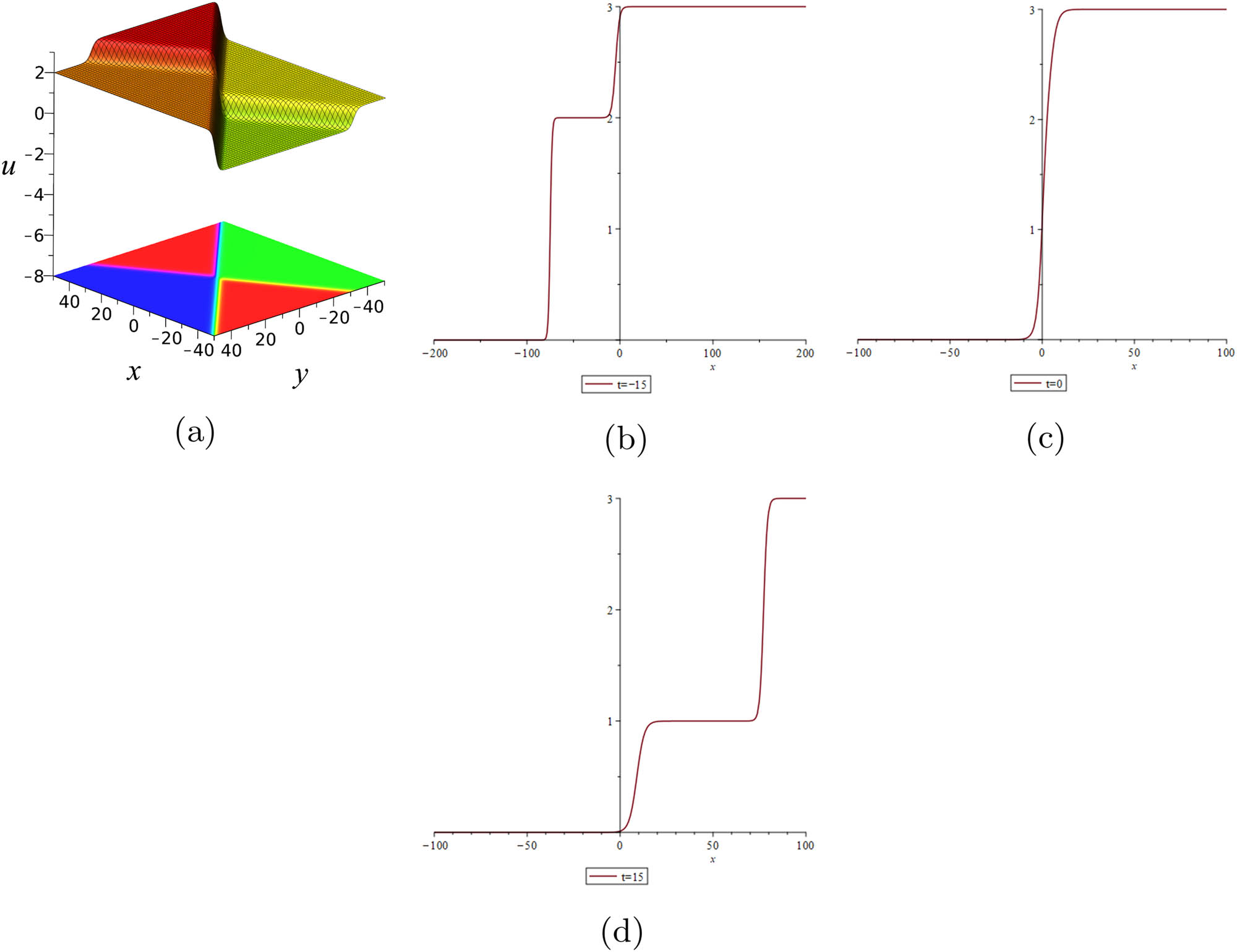
As shown in Figure 1, the 1-soliton propagates in the positive direction along the Y -axis. During propagation, the soliton can maintain its shape and speed without significant attenuation or deformation, even over long distances. The soliton model can help understand and predict the behavior of catastrophic water waves, such as tsunamis.

Figure 1

1-soliton wave solution. (a)–(c) show the three-dimensional plot and density plot of the ( x , y ) plane for t = − 15 , 0, and 15, respectively.

3.2 2-soltion solution

To investigate the 2-soltion solution, setting N = 2 , Eq. (16) can be expressed in the following manner:

(19) f = 1 + e ξ 1 + e ξ 2 + A 12 e ξ 1 + ξ 2 ,

where ξ i = k i τ + μ i t + η i x + ω i y + λ i z + η i 0 .

By substituting Eq. (19) into bilinear Eq. (12), we obtain the relation among k i and μ i as follows:

(20) k i = η i 3 , μ i = − η i 2 ω i − η i λ − μ ω i − ν λ i , A 12 = ( η 1 − η 2 ) 2 ( η 1 + η 2 ) 2 ,

where i = 1 , 2.

Letting the parameters λ = 1 , μ = 2 , ν = 2 , η 1 = 0.5 , η 2 = 1 , λ 1 = 0.8 , λ 2 = 0.5 , ω 1 = − 0.8 , ω 2 = 1 , and η i 0 = 0 , substituting Eq. (19) into Eq. (14), we obtain the 2-soliton solution of Eq. (5).

As shown in Figure 2, at t = − 15 , two solitons propagate independently, each preserving its distinct shape. When they intersect, they undergo intense nonlinear interactions, which cause notable changes in their waveforms and may lead to overlapping and the formation of intricate patterns. By t = 15 , solitons continue their travel, returning to their original shapes as they move apart. This dynamic behavior highlights the solitons’ resilience and interaction characteristics.

Figure 2

2-soliton wave solution. (a) show the three-dimensional plot and density plot of the ( x , y ) plane. (b)–(d) show the two-dimensional plot of the x plane for t = − 15 , 0, and 15, respectively.

3.3 3-soltion solution

To investigate the 3-soltion solution, setting N = 3 , Eq. (16) can be expressed in the following manner:

(21) f = 1 + e ξ 1 + e ξ 2 + e ξ 3 + A 12 e ξ 1 + ξ 2 + A 13 e ξ 1 + ξ 3 + A 23 e ξ 2 + ξ 3 + A 12 A 13 A 23 e ξ 1 + ξ 2 + ξ 3 ,

where A i j = ( η i − η j ) 2 ( η i + η j ) 2 .

Substituting Eq. (21) into bilinear Eq. (12), letting the parameters η 1 = 1.4 , η 3 = 0.4 , η 2 = 1.2 , ω 1 = 1 , ω 3 = 2 , ω 2 = 2.5 , λ 1 = 1 , λ 2 = 2.5 , λ 3 = 3 , λ = 1 , μ = 1 , ν = 2 , and η i 0 = 0 , and substituting Eq. (21) into Eq. (14), we obtain the 3-soliton solution of Eq. (5).

According to Figure 3, the dynamic behavior of the 3-soliton solution closely resembles that of the 2-soliton solution. The solitons maintain their shapes before and after interaction, demonstrating stability and persistence in their form throughout the process. This behavior illustrates the characteristic resilience of solitons in maintaining their structure despite complex interactions.

Figure 3

3-soliton wave solution. (a) show the three-dimensional plot and density plot of the ( x , y ) plane. (b)–(d) show the two-dimensional plot of the x plane for t = − 15 , − 6 , and 2, respectively.

4 Conclusions

In this article, we examined the (3+1)-dimensional negative-order KdV-CBS equation, a widely used mathematical and physical model for describing multiwave interactions with significant physical implications. This equation generalizes the KdV equation, extending its applicability to more complex systems, including interactions in higher dimensions. It provides a valuable framework for understanding phenomena such as wave propagation, soliton behavior, and nonlinear interactions in fields like fluid dynamics, plasma physics, and optical systems.

We observed that for specific parameter values, the equation reduces to well-known forms: when μ = ν = 0 , (5) simplifies to (3), and when λ = ν = 0 , (5) simplifies to (4). These reductions offer insights into the relationships between different forms of the equation and allow for a clearer analysis of how various terms influence the system’s dynamics.

A major contribution of this work is the application of binary Bell polynomials to the (3+1)-dimensional negative-order KdV-CBS equation. This approach enables the transformation of the equation into its bilinear form, following a detailed derivation process. The bilinear form is especially beneficial as it simplifies the nonlinear terms, facilitating analysis and solution finding. Through this transformation, we not only derive explicit solutions but also gain a deeper understanding of the equation’s structure and behavior, thus opening new avenues for studying complex nonlinear equations.

By using the bilinear form, we successfully derived 1-soliton, 2-soliton, and 3-soliton solutions. Solitons, which are stable wave packets that maintain their shape during propagation, play a crucial role in many physical systems. The soliton solutions obtained demonstrate the intricate behaviors that arise from the equation, including interactions between solitons and the patterns they form. Studying soliton solutions is particularly important as solitons appear in various fields, ranging from water waves to optical fibers. Understanding their interactions in higher dimensions can offer valuable insights into more complex systems, such as wave interactions in multidimensional media.

The results of this study contribute to a broader understanding of nonlinear wave equations and soliton theory. By applying binary Bell polynomials to this class of equations, we demonstrated a systematic approach to their analysis and solution. This method can be extended to other nonlinear equations, particularly those in higher dimensions, where traditional solution methods may prove less effective.

Future research could expand upon these findings by exploring the application of binary Bell polynomials to more complex equations, such as those involving higher-order derivatives or additional nonlinear terms. Furthermore, the soliton solutions derived in this article could be further studied to understand their stability, interactions, and potential for describing real-world phenomena. For instance, researchers might examine how solitons behave under perturbations or how they evolve over longer timescales.

In conclusion, this work presents a thorough analysis of the (3+1)-dimensional negative-order KdV-CBS equation using binary Bell polynomials, contributing to the growing body of knowledge on multiwave interactions and soliton theory. We hope that the results obtained here will be valuable to researchers interested in nonlinear wave equations and their applications across various scientific and engineering fields. The methods and solutions presented in this article pave the way for future studies on higher-dimensional systems and more complex mathematical models.

References

[1] Dysthe K, Krogstad HE, Muller P. Oceanic rogue waves. An Rev Fluid Mech. 2008;40(1):287–310. 10.1146/annurev.fluid.40.111406.102203Search in Google Scholar
[2] Alkhidhr HA, Abdelrahman MA. Wave structures to the three couplednonlinear Maccarias systems in plasma physics. Results Phys. 2022;33:105092. 10.1016/j.rinp.2021.105092Search in Google Scholar
[3] Javed F, Rani B, Chahlaoui Y, Baskonus HM, Raza N. Nonlinear dynamics of wave structures for the Davey-Stewartson system: a truncatedPainlevé approach. Nonlinear Dynam. 2024;112(24):22189–200. 10.1007/s11071-024-10189-7Search in Google Scholar
[4] Zhao XH, Li SX. Dark soliton solutions for a variable coefficient higher-order Schrödinger equation in the dispersion decreasing fibers. Appl Math Lett. 2022;132:108159. 10.1016/j.aml.2022.108159Search in Google Scholar
[5] Fan LL, Bao T. The integrability and infinite conservation laws of a variable coefficient higher-order Schrödinger equation. Chinese J Phys. 2024;90:753–63. 10.1016/j.cjph.2024.06.010Search in Google Scholar
[6] Chen D, Shi D, Chen F. Qualitative analysis and new traveling wave solutions for the stochastic Biswas-Milovic equation. AIMS Math. 2025;10:4092–119. 10.3934/math.2025190Search in Google Scholar
[7] Fan EG. Extended tanh-function method and its applications to nonlinear equations. Phys Lett A. 2000;277(4–5):212–8. 10.1016/S0375-9601(00)00725-8Search in Google Scholar
[8] He JS, Zhang L, Cheng Y, Li YS. Determinant representation of daroboux transformation for the akns system. SCI China Ser A. 2006;49:1867–78. 10.1007/s11425-006-2025-1Search in Google Scholar
[9] Yin TL, Xing ZP, Pang J. Modified Hirota bilinear method to (3+1)-D variable coefficients generalized shallow water wave equation. Nonlinear Dynam. 2023;111(11):9741–52. 10.1007/s11071-023-08356-3Search in Google Scholar
[10] Zhang RF, Li MC, Gan JY, Li Q, Lan ZZ. Novel trial functions and rogue waves of generalized breaking soliton equation via bilinear neural network method. Chaos Solitons Fract. 2022;154:111692. 10.1016/j.chaos.2021.111692Search in Google Scholar
[11] Zhong J, Ma ZM, Lei R, Liang J, Wang Y. Dynamics of heterotypic soliton, high-order breather, m-lump wave, and multi-wave interaction solutions for a (3+1)-dimensional Kadomtsev-Petviashvili equation. Eur Phys J Plus. 2024;139(3):1–16. 10.1140/epjp/s13360-024-05082-6Search in Google Scholar
[12] Wahlquist HD, Estabrook FB. Bäcklund transformation for solutions of the Korteweg-de Vries equation. Phys Rev Lett. 1973;31(23):1386. 10.1103/PhysRevLett.31.1386Search in Google Scholar
[13] Bailung H, Sharma S, Nakamura Y. Observation of peregrine solitons in a multicomponent plasma with negative ions. Phys Rev Lett. 2011;107(25):255005. 10.1103/PhysRevLett.107.255005Search in Google Scholar PubMed
[14] Kibler B, Fatome J, Finot C, Millot G, Dias F, Genty G, et al. The peregrine soliton in nonlinear fibre optics. Nature Phys. 2010;6(10):790–5. 10.1038/nphys1740Search in Google Scholar
[15] Helal M. Soliton solution of some nonlinear partial differential equations and its applications in fluid mechanics. Chaos Solitons Fract. 2002;13(9):1917–29. 10.1016/S0960-0779(01)00189-8Search in Google Scholar
[16] Hirota R. Exact solution of the Korteweg–de Vries equation for multiple collisions of solitons. Phys Rev Lett. 1971;27(18):1192. 10.1103/PhysRevLett.27.1192Search in Google Scholar
[17] Wazwaz AM. A new (2+1)-dimensional Korteweg-de Vries equation and its extension to a new (3+1)-dimensional Kadomtsev-Petviashvili equation. Phys Scr. 2011;84(3):035010. 10.1088/0031-8949/84/03/035010Search in Google Scholar
[18] Kouichi T, Yu SJ, Takeshi F. The Bogoyavlenskii-Schiff hierarchy and integrable equations in (2+1) dimensions. Rep Math Phys. 1999;44(1–2):247–54. 10.1016/S0034-4877(99)80166-9Search in Google Scholar
[19] Wazwa AM. Abundant solutions of various physical features for the (2+1)-dimensional modified KdV-Calogero-Bogoyavlenskii-Schiff equation. Nonlinear Dynam. 2017;89(3):1727–32. 10.1007/s11071-017-3547-5Search in Google Scholar
[20] Wazwaz AM. Two new painlevé integrable KdV-Calogero-Bogoyavlenskii-Schiff (KdV-CBS) equation and new negative-order KdV-CBS equation. Nonl Dynam. 2021;104(4):4311–5. 10.1007/s11071-021-06537-6Search in Google Scholar
[21] Raza N, Arshed S, Kaplan M. Multiple soliton and traveling wave solutions for the negative-order-KdV-CBS model. Rev Mex Fís. 2024;70:031305. 10.31349/RevMexFis.70.031305Search in Google Scholar
[22] Miguel VC, Beenish R, Nauman R, Ali BG, Mudassar I. An exploration of the (3+1)-dimensional negative order KdV-CBS model: Wave solutions, Bäcklund transformation, and complexiton dynamics. PLoS One. 2024;19(4):0296978. 10.1371/journal.pone.0296978Search in Google Scholar PubMed PubMed Central
[23] Guo XY, Li LZ. Auto-Bäcklund transformation and exact solutions for a new integrable (3+1)-dimensional KdV-CBS equation. Qual Theor Dyn Syst. 2024;23(5):207. 10.1007/s12346-024-01062-4Search in Google Scholar
[24] Xu GQ, Wazwaz AM. Characteristics of integrability, bidirectional solitons and localized solutions for a (3+1)-dimensional generalized breaking soliton equation. Nonlinear Dynam. 2019;96(3):1989–2000. 10.1007/s11071-019-04899-6Search in Google Scholar
[25] Lan ZZ, Dong S, Gao B, Shen YJ. Bilinear form and soliton solutions for a higher order wave equation. Appl Math Lett. 2022;134:108340. 10.1016/j.aml.2022.108340Search in Google Scholar
[26] Lambert F, Loris I, Springael J, Willer R. On a direct bilinearization method: Kaupas higher-order water wave equation as a modified nonlocal Boussinesq equation. J Phys A Math Gen. 1994;27(15):5325. 10.1088/0305-4470/27/15/028Search in Google Scholar
[27] Ma ZM, Wang BJ, Liu XK, Liu YL. Bäcklund transformation, lax pair and dynamic behaviour of exact solutions for a (3+1)-dimensional nonlinear equation. Pramana. 2024;98(1):24. 10.1007/s12043-023-02721-ySearch in Google Scholar
[28] Lü X, Tian B, Sun K, Wang P. Bell-polynomial manipulations on the Bäcklund transformations and lax pairs for some soliton equations with one tau-function. J Math Phys. 2010;51(11):113506. 10.1063/1.3504168Search in Google Scholar
[29] Lü X, Tian B, Qi FH. Bell-polynomial construction of Bäcklund transformations with auxiliary independent variable for some soliton equations with one Tau-function. Nonlinear Anal Real. 2012;13(3):1130–8. 10.1016/j.nonrwa.2011.09.006Search in Google Scholar
© 2025 the author(s), published by De Gruyter
This work is licensed under the Creative Commons Attribution 4.0 International License.
Articles in the same Issue
- Research Articles
- Single-step fabrication of Ag2S/poly-2-mercaptoaniline nanoribbon photocathodes for green hydrogen generation from artificial and natural red-sea water
- Abundant new interaction solutions and nonlinear dynamics for the (3+1)-dimensional Hirota–Satsuma–Ito-like equation
- A novel gold and SiO2 material based planar 5-element high HPBW end-fire antenna array for 300 GHz applications
- Explicit exact solutions and bifurcation analysis for the mZK equation with truncated M-fractional derivatives utilizing two reliable methods
- Optical and laser damage resistance: Role of periodic cylindrical surfaces
- Numerical study of flow and heat transfer in the air-side metal foam partially filled channels of panel-type radiator under forced convection
- Water-based hybrid nanofluid flow containing CNT nanoparticles over an extending surface with velocity slips, thermal convective, and zero-mass flux conditions
- Dynamical wave structures for some diffusion--reaction equations with quadratic and quartic nonlinearities
- Solving an isotropic grey matter tumour model via a heat transfer equation
- Study on the penetration protection of a fiber-reinforced composite structure with CNTs/GFP clip STF/3DKevlar
- Influence of Hall current and acoustic pressure on nanostructured DPL thermoelastic plates under ramp heating in a double-temperature model
- Applications of the Belousov–Zhabotinsky reaction–diffusion system: Analytical and numerical approaches
- AC electroosmotic flow of Maxwell fluid in a pH-regulated parallel-plate silica nanochannel
- Interpreting optical effects with relativistic transformations adopting one-way synchronization to conserve simultaneity and space–time continuity
- Modeling and analysis of quantum communication channel in airborne platforms with boundary layer effects
- Theoretical and numerical investigation of a memristor system with a piecewise memductance under fractal–fractional derivatives
- Tuning the structure and electro-optical properties of α-Cr2O3 films by heat treatment/La doping for optoelectronic applications
- High-speed multi-spectral explosion temperature measurement using golden-section accelerated Pearson correlation algorithm
- Dynamic behavior and modulation instability of the generalized coupled fractional nonlinear Helmholtz equation with cubic–quintic term
- Study on the duration of laser-induced air plasma flash near thin film surface
- Exploring the dynamics of fractional-order nonlinear dispersive wave system through homotopy technique
- The mechanism of carbon monoxide fluorescence inside a femtosecond laser-induced plasma
- Numerical solution of a nonconstant coefficient advection diffusion equation in an irregular domain and analyses of numerical dispersion and dissipation
- Numerical examination of the chemically reactive MHD flow of hybrid nanofluids over a two-dimensional stretching surface with the Cattaneo–Christov model and slip conditions
- Impacts of sinusoidal heat flux and embraced heated rectangular cavity on natural convection within a square enclosure partially filled with porous medium and Casson-hybrid nanofluid
- Stability analysis of unsteady ternary nanofluid flow past a stretching/shrinking wedge
- Solitonic wave solutions of a Hamiltonian nonlinear atom chain model through the Hirota bilinear transformation method