Nonclassical correlation dynamics of Heisenberg XYZ states with (x, y)-spin--orbit interaction, x-magnetic field, and intrinsic decoherence effects
-
Fahad Aljuaydi
 ,
Sattam N. Almutairi
,
Sattam N. Almutairi

Abstract
In quantum information, it is important to recognize the effects of additional interactions, such as spin–orbit interactions, on the quantum information resources of two-qubit Heisenberg states. Therefore, we study the nonlocal correlation dynamics affected by the intrinsic decoherence of the spin–spin-Heisenberg-XYZ interaction, which is supported by spin–orbit interactions (Dzyaloshinsky–Moriya) of the
1 Introduction
Among the various quantum systems proposed for implementing quantum information and computation [1,2], superconducting circuits, trapped ions, and semiconductor quantum dots are crucial techniques for realizing quantum bits (qubits). Based on electron spins trapped in quantum dots, a quantum computer protocol has been initially proposed [3–5]. The electron, having a spin of (
Exploring two-qubit information dynamics in various proposed qubit systems, based on different types of nonlocal correlations (NLCs) (such as entanglement and quantum discord), is one of the most critical research fields in implementing quantum information and computation [28]. Quantum entanglement (QE), quantified by measures such as entropy [29], concurrence [30], negativity, and log-negativity [31], is a significant type of two-qubit NLCs [32,33]. It has a wide range of applications in quantum information fields, including quantum computation, teleportation [34,35], quantum optical memory [36], and quantum key distribution [37]. After implementing quantum discord as another type of qubits’ NLCs beyond entanglement [38], several quantifiers have been introduced to address other NLCs [39] using Wigner–Yanase (WY) skew information [40] and quantum Fisher information (QFI) [41]. WY-skew-information minimization (local quantum uncertainty, LQU) [42] and WY-skew-information maximization (uncertainty-induced nonlocality) [43] have been introduced to quantify other NLCs beyond entanglement. Additionally, the minimization of QFI (local quantum Fisher information, LQFI) has been used to implement another two-qubit NLC [44,45]. LQU has a direct connection to LQFI [46,47], establishing more two-qubit NLCs in several proposed qubit systems [48], such as hybrid–spin systems (under random noise [49] and intrinsic decoherence [50]), two-coupled double quantum dots [51], the mixed-spin Heisenberg model [52], and the Heisenberg system [53].
The information dynamics of two-spin Heisenberg XYZ states have been investigated using the Milburn intrinsic decoherence model [54]. This includes studies on entanglement teleportation based on the Heisenberg XYZ chain [24,55], the LQFI of Heisenberg XXX states beyond IEMF effects [56], and quantum correlations of concurrence and LQU [57]. Previous works have focused on exploring the time evolution of the two-spin Heisenberg XYZ states’ NLCs under limited conditions on spin–spin and spin–orbit interactions, as well as applied magnetic fields, to ensure residing quantum information resources of two-qubit
Motivated by the aforementioned experimental evidence for realizations for the spin–orbit interaction having a high ability to support the generating NLCs, and the importance of general two-qubit Heisenberg states, this study employs the Milburn intrinsic decoherence and Heisenberg XYZ models to explore the NLC dynamics of LQFI, LQU, and log-negativity for general two-qubit Heisenberg XYZ states with non-
The manuscript structure includes the Milburn intrinsic decoherence equation, the Heisenberg XYZ model, and its solution in Section 2. In Section 3, we introduce the definitions of the NLCs’ quantifiers: LQFI, LQU, and LN. Section 4 presents the outcomes of the dependence of these quantifiers on the physical parameters. Our conclusions are provided in Section 5.
2 Heisenberg spin model
Here, the Milburn intrinsic decoherence and Heisenberg XYZ models are used to examine the capabilities embedded in spin–spin interaction supported by the spin–orbit (Dzyaloshinsky–Moriya) interactions in the
where
In the two-spin–qubits basis:
with
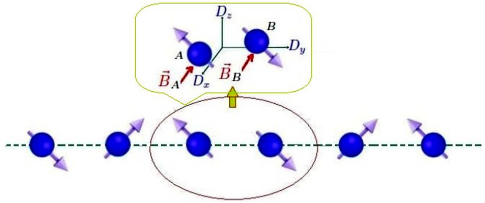
Diagram of a Heisenberg XYZ chain model, where two arbitrary spin–qubits (
The time evolution of the NLCs in the generated two spin–qubit states, represented by the density matrix
where
After calculating the eigenvalues
This solution depends on the unitary interaction
Eq. (5) is used to numerically calculate and explore the dynamics of the NLCs within the two-spin–qubit states’ Heisenberg XYZ model under the effects of spin–orbit interactions along the
3 NLC quantifiers
Here, the two-spin NLCs will be measured by the following quantifiers: LQFI, LQU, and LN.
LQFI
Here, we use LQFI to quantify another type of two-spin Heisenberg-XYZ correlation beyond entanglement. After calculating the two-spin eigenvalues
which depends on the highest eigenvalue
For a maximally correlated two-spin–qubit state, the LQFI function converges to
LQU
Also, we use LQU of WY skew information [40] to realize another type of two-spin–qubits’ NLC [40,42,43]. For the two-spin density matrix
(7)which depends on the largest eigenvalue
The LQU function oscillates and is bounded by the inequality
Logarithmic negativity (LN)
We employ LN [31] to measure the generated two-spin–qubit entanglement. The LN expression is based on the negativity’s definition
(8)The LN function vanishes,
In the following, we work in a system of units where
4 Two-spin qubit dynamics
To explore the generation of non-local correlations between two spin qubits, we consider that the two spins are initially in their uncorrelated upper states
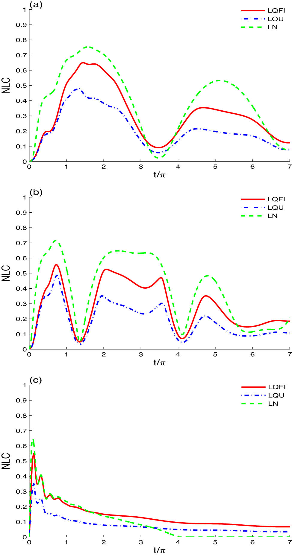
Our first analysis, starting from Figure 2, illustrates the dynamics of non-local correlations (LQFI, LQU, and LN) between two spin qubits. These correlations are generated by the couplings
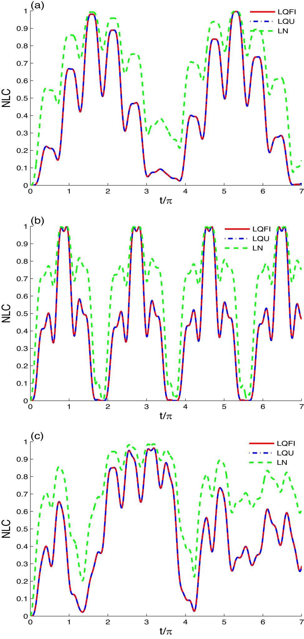
Time evolution of the LQFI, LQU, and LN are shown with the two-spin couplings
The
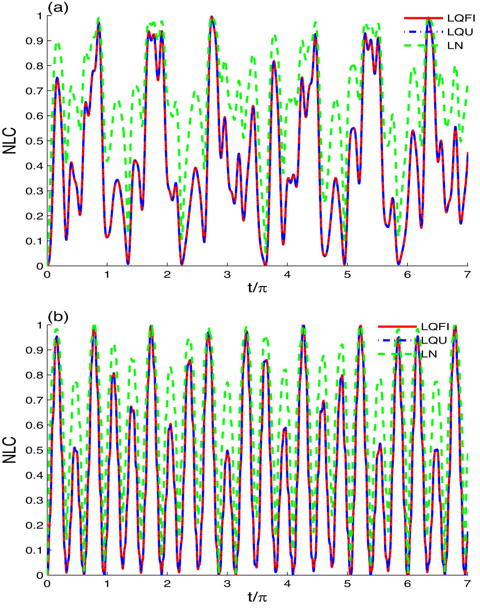
Figure 3(a) and (b) illustrates that higher spin–spin interaction couplings (
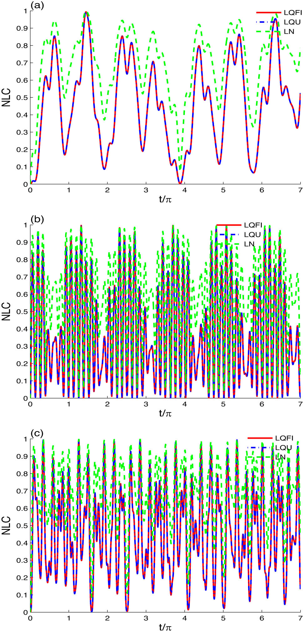
Time evolution of the LQFI, LQU, and LN of Figure 2(c) are plotted for different two-spin couplings:
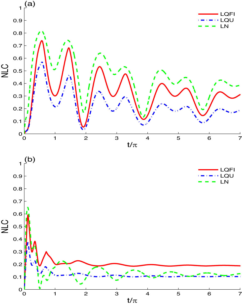
Figure 4 illustrates the LQFI–LQU correlation and log-negativity entanglement dynamics of Figure 3(a) (where
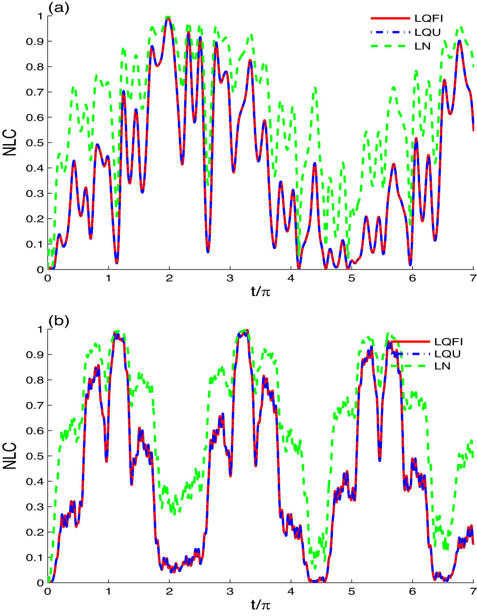
Time evolutions of LQFI, LQU, and LN of Figure 3(a) (for
In the upcoming analysis of Figure 5, we maintain the same parameter values as in Figure 3a (with
Time evolutions of LQFI, LQU, and LN of Figure 3(a) (for
The next illustrations in Figures 6, 7, 8 depict the time evolutions of NLCs of LQFI, LQU, and log-negativity in the presence of non-zero ISSD coupling. By comparing the results of Figure 2(a) (
Time evolutions of LQFI, LQU, and LN of Figure 2(a) are shown in the presence of the ISSD effect (
Time evolutions of LQFI, LQU, and LN of Figure 6(b) and (c) are shown but for strong spin–spin couplings with
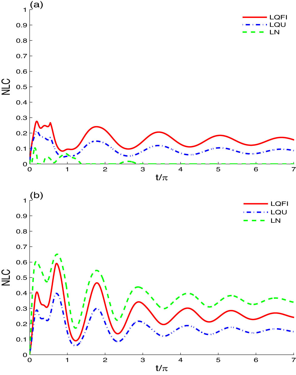
Time evolutions of LQFI, LQU, and LN in Figure 4(a), for
As shown in Figure 6(b) and (c), increasing the intensities of
Figure 7 illustrates the time evolutions of LQFI, LQU, and LN of Figure 6(b) and (c), but for strong spin–spin couplings with
Figure 8(a) shows the time evolutions of LQFI, LQU, and LN from Figure 4(a) for
5 Conclusion
In this study, we use the Milburn intrinsic decoherence and the Heisenberg XYZ models to explore the capabilities of spin–spin and spin–orbit interactions (in the
Acknowledgments
The author is very grateful to the referees and the associate editor for their important remarks which have helped him to improve the manuscript. This study is supported via funding from Prince sattam bin Abdulaziz University Project Number (PSAU/2025/R/1446).
-
Funding information: This study was funded by Princess Nourah bint Abdulrahman University Researchers Supporting Project Number (PNURSP2025R906), Princess Nourah bint Abdulrahman University, Riyadh, Saudi, Arabia.
-
Author contributions: Sattam N. Almutairi, Heba Allhibi, and Fahad Aljuaydi prepared all the figures and performed the mathematical calculations. Heba Allhibi, Sattam N. Almutairi, and Fahad Aljuaydi wrote the original draft. Abdel-Baset A. Mohamed, Sattam N. Almutairi, and Fahad Aljuaydi reviewed and edited the draft. All authors have accepted responsibility for the entire content of this manuscript and approved its submission.
-
Conflict of interest: The authors state no conflict of interest.
-
Data availability statement: The datasets generated during and/or analysed during the current study are available from the corresponding author on reasonable request.
References
[1] Horodecki R, Horodecki P, Horodecki M, Horodecki K. Quantum entanglement. Rev Mod Phys. 2009;81:865. 10.1103/RevModPhys.81.865Search in Google Scholar
[2] Nielsen MA, Chuang IL. Quantum computation and quantum information. Cambridge: Cambridge University Press; 2000. Search in Google Scholar
[3] Loss D, DiVincenzo DP. Quantum computation with quantum dots. Phys Rev A 1998;57:120. 10.1103/PhysRevA.57.120Search in Google Scholar
[4] Burkard G, Loss D, DiVincenzo DP. Coupled quantum dots as quantum gates. Phys Rev B. 1999;59:2070. 10.1103/PhysRevB.59.2070Search in Google Scholar
[5] Vandersypen LMK, Hanson R, van Willems Beveren LH, Elzerman JM, Greidanus JS, De Franceschi S, et al. Quantum computing and quantum bits in mesoscopic systems. Boston, M A.: Springer; 2004. Search in Google Scholar
[6] Ma R-L, Li A-R, Wang C, Kong ZZ, Liao W-Z, Ni M, et al. Single-spin–qubit geometric gate in a silicon quantum dot. Phys Rev Appl. 2024;21:014044. 10.1103/PhysRevApplied.21.014044Search in Google Scholar
[7] Zwolak JP, Taylor JM. Colloquium: Advances in automation of quantum dot devices control. Rev Mod Phys. 2023;95:011006. 10.1103/RevModPhys.95.011006Search in Google Scholar PubMed PubMed Central
[8] Pinheiro F, Bruun GM, Martikainen J-P, Larson J. XYZ Quantum Heisenberg Models with p-Orbital Bosons. Phys Rev Lett. 2013;111:205302. 10.1103/PhysRevLett.111.205302Search in Google Scholar PubMed
[9] Bermudez A, Tagliacozzo L, Sierra G, Richerme P. Long-range Heisenberg models in quasiperiodically driven crystals of trapped ions. Phys Rev B Condens Matter Mater Phys. 2017;95:024431. 10.1103/PhysRevB.95.024431Search in Google Scholar
[10] Nishiyama M, Inada Y, Zheng GQ. Spin triplet superconducting state due to broken inversion symmetry in Li2Pt3B. Phys Rev Lett. 2007;98:047002. 10.1103/PhysRevLett.98.047002Search in Google Scholar PubMed
[11] Yue W, Wei Q, Kais S, Friedrichc B, Herschbach D. Realization of Heisenberg models of spin systems with polar molecules in pendular states. Phys Chem Chem Phys. 2022;24:25270. 10.1039/D2CP00380ESearch in Google Scholar PubMed
[12] Dzyaloshinski I. A thermodynamic theory of “weak” ferromagnetism of antiferromagnetics. J Phys Chem Solids. 1958;4:241. 10.1016/0022-3697(58)90076-3Search in Google Scholar
[13] Moriya T. Theory of Magnetism of NiF2. Phys Rev. 1960;117:635. 10.1103/PhysRev.117.635Search in Google Scholar
[14] Moriya T. New mechanism of anisotropic superexchange interaction. Phys Rev Lett. 1960;4:228. 10.1103/PhysRevLett.4.228Search in Google Scholar
[15] Shekhtman L, Entin-Wohlman O, Aharony A. Bond-dependent symmetric and antisymmetric superexchange interactions in La2CuO4. Phys Rev B. 1993;47:174. 10.1103/PhysRevB.47.174Search in Google Scholar
[16] Moriya T. Anisotropic superexchange interaction and weak Ferromagnetism. Phys Rev. 1960;120:91. 10.1103/PhysRev.120.91Search in Google Scholar
[17] Kuznetsova EI, Yurischev MA. Quantum discord in spin systems with dipole-dipole interaction. Quantum Inf Process. 2013;12:3587–605. 10.1007/s11128-013-0617-6Search in Google Scholar
[18] Arnesen MC, Bose S, Vedral V. Natural thermal and magnetic entanglement in the 1D Heisenberg model. Phys Rev Lett. 2001;87:017901. 10.1103/PhysRevLett.87.017901Search in Google Scholar PubMed
[19] Li D-C, Cao Z-L. Thermal entanglement in the anisotropic Heisenberg (XYZ) model with different inhomogeneous magnetic fields. Optics Commun. 2009;282:1226–30. 10.1016/j.optcom.2008.11.087Search in Google Scholar
[20] Matthies T, Rózsa L, Szunyogh L, Wiesendanger R, Vedmedenko EY. Interlayer and interfacial Dzyaloshinskii-Moriya interaction in magnetic trilayers: First-principles calculations. Phys Rev Res. 2024;6:043158. 10.1103/PhysRevResearch.6.043158Search in Google Scholar
[21] Thoma H, Hutanu V, Deng H, Dmitrienko VE, Brown PJ, Gukasov A, et al. Revealing the absolute direction of the Dzyaloshinskii-Moriya interaction in prototypical weak ferromagnets by polarized neutrons. Phys Rev X. 2021;11:011060. 10.1103/PhysRevX.11.011060Search in Google Scholar
[22] Zhao HJ, Chen P, Prosandeev S, Artyukhin S, Bellaiche L. Dzyaloshinskii-Moriya-like interaction in ferroelectrics and antiferroelectrics. Nature Materials. 2021;20:341. 10.1038/s41563-020-00821-3Search in Google Scholar PubMed
[23] Allenspach R, Bischof A, Boehm B, Drechsler U, Reich O, Sousa M, et al. Dzyaloshinskii-Moriya interaction in Ni/Cu(001). Phys Rev B. 2024;110:014402. 10.1103/PhysRevB.110.014402Search in Google Scholar
[24] Hosseiny SM, Seyed-Yazdi J, Norouzi M, Livreri P. Quantum teleportation in Heisenberg chain with magnetic-field gradient under intrinsic decoherence. Sci Rep. 2024;14:9607. 10.1038/s41598-024-60321-1Search in Google Scholar PubMed PubMed Central
[25] Khedif Y, Muthuganesan R. Intrinsic decoherence dynamics and dense coding in dipolar spin system. Appl Phys B. 2023;129:19. 10.1007/s00340-022-07956-ySearch in Google Scholar
[26] Abd-Rabbou MY, ur Rahman A, Yurischev MA, Haddadi S. Comparative study of quantum Otto and Carnot engines powered by a spin working substance. Phys Rev E. 2023;108:034106. 10.1103/PhysRevE.108.034106Search in Google Scholar PubMed
[27] Yurischev MA. On the quantum correlations in two-qubit XYZ spin chains with Dzyaloshinsky–Moriya and Kaplan–Shekhtman–Entin-Wohlman–Aharony interactions. Quantum Inf Process. 2020;19:336. 10.1007/s11128-020-02835-xSearch in Google Scholar
[28] Le Bellac M. A short introduction to quantum information and quantum computation. Cambridge: Cambridge University Press; 2006. 10.1017/CBO9780511755361Search in Google Scholar
[29] Eisert J, Cramer M, Plenio MB. Colloquium: Area laws for the entanglement entropy. Rev Mod Phys. 2010;82:277. 10.1103/RevModPhys.82.277Search in Google Scholar
[30] Wootters WK. Entanglement of formation of an arbitrary state of two qubits. Phys Rev Lett. 1998;80:2245. 10.1103/PhysRevLett.80.2245Search in Google Scholar
[31] Vidal G, Werner RF. Computable measure of entanglement. Phys Rev A. 2002;65:032314. 10.1103/PhysRevA.65.032314Search in Google Scholar
[32] Eftekhari F, Tavassoly MK, Behjat A, Faghihi MJ. Entanglement and atomic inversion in a dissipative two-atom-optomechanical system. Optics Laser Tech. 2024;168:109934. 10.1016/j.optlastec.2023.109934Search in Google Scholar
[33] Abdel-Wahab NH, Zangi SM, Seoudy TA, Haddadi S. Dynamical evolution of a five-level atom interacting with an intensity-dependent coupling regime influenced by a nonlinear Kerr-like medium. Sci Rep. 2024;14:25211. 10.1038/s41598-024-76629-xSearch in Google Scholar PubMed PubMed Central
[34] Braunstein SL, Kimble HJ. Teleportation of continuous quantum variables. Phys Rev Lett. 1998;80:869. 10.1103/PhysRevLett.80.869Search in Google Scholar
[35] Bouwmeester D, Pan JW, Mattle K, Eibl M, Weinfurter H, Zeilinger A. Experimental quantum teleportation. Nature. 1997;390:575. 10.1038/37539Search in Google Scholar
[36] Lei Y, Asadi FK, Zhong T, Kuzmich A, Simon C, Hosseini M. Quantum optical memory for entanglement distribution. Optica. 2023;10:1511–28. 10.1364/OPTICA.493732Search in Google Scholar
[37] Ekert AK. Quantum cryptography based on Bell’s theorem. Phys Rev Lett. 1991;67:661. 10.1103/PhysRevLett.67.661Search in Google Scholar PubMed
[38] Ollivier H, Zurek WH. Quantum discord: A measure of the quantumness of correlations. Phys Rev Lett. 2001;88:017901. 10.1103/PhysRevLett.88.017901Search in Google Scholar PubMed
[39] Hu M-L, Hu X, Wang J, Peng Y, Zhang Y-R, Fan H. Quantum coherence and geometric quantum discord. Phys Rep. 2018;762:1. 10.1016/j.physrep.2018.07.004Search in Google Scholar
[40] Wigner EP, Yanase MM. Information contents of distributions. Proc Natl Acad Sci. 1963;49:910. 10.1073/pnas.49.6.910Search in Google Scholar PubMed PubMed Central
[41] Girolami D, Souza AM, Giovannetti V, Tufarelli T, Filgueiras JG, Sarthour RS, et al. Quantum discord determines the interferometric power of quantum states. Phys Rev Lett. 2014;112:210401. 10.1103/PhysRevLett.112.210401Search in Google Scholar
[42] Girolami D, Tufarelli T, Adesso G. Characterizing nonclassical correlations via local quantum uncertainty. Phys Rev Lett. 2013:110:240402. 10.1103/PhysRevLett.110.240402Search in Google Scholar PubMed
[43] Wu S-X, Zhang J, Yuuu C-S, Song H-S. Uncertainty-induced quantum nonlocality. Phys Lett A. 2014;378:344. 10.1016/j.physleta.2013.11.047Search in Google Scholar
[44] Dhar HS, Bera MN, Adesso G. Characterizing non-Markovianity via quantum interferometric power. Phys Rev A. 2015;991:032115. 10.1103/PhysRevA.91.032115Search in Google Scholar
[45] Kim S, Li L, Kumar A, Wu J. Characterizing nonclassical correlations via local quantum Fisher information. Phys Rev A. 2018;97:032326. 10.1103/PhysRevA.97.032326Search in Google Scholar
[46] Helstrom CW. Quantum detection and estimation theory. New York: Academic; 1976. Search in Google Scholar
[47] Paris MGA. Quantum estimation for quantum technology. Int J Quant Inf. 2009;7:125. 10.1142/S0219749909004839Search in Google Scholar
[48] Mohamed A-B A, Farouk A, Yassen MF, Eleuch H. Fisher and skew information correlations of two coupled trapped ions: Intrinsic decoherence and Lamb-Dicke nonlinearity. Symmetry. 2021;13:2243. 10.3390/sym13122243Search in Google Scholar
[49] Benabdallah F, Ur Rahman A, Haddadi S, Daoud M. Long-time protection of thermal correlations in a hybrid-spin system under random telegraph noise. Phys Rev E. 2022;106:034122. 10.1103/PhysRevE.106.034122Search in Google Scholar PubMed
[50] Benabdallah F, El Anouz K, Ur Rahman A, Daoud M, El Allati A, Haddadi S. Witnessing quantum correlations in a hybrid Qubit-Qutrit system under intrinsic decoherence. Fortschr Phys. 2023;71:2300032. 10.1002/prop.202300032Search in Google Scholar
[51] Elghaayda S, Dahbi Z, Mansour M. Local quantum uncertainty and local quantum Fisher information in two-coupled double quantum dots. Opt Quant Electron 2022;54:419. 10.1007/s11082-022-03829-ySearch in Google Scholar
[52] Wei P-F, Luo Q, Wang H-Q-C, Xiong S-J, Liu B, Sun Z. Local quantum Fisher information and quantum correlation in the mixed-spin Heisenberg XXZ chain. Front Phys. 2024;19:21201. 10.1007/s11467-023-1336-9Search in Google Scholar
[53] Fedorova AV, Yurischev MA. Behavior of quantum discord, local quantum uncertainty, and local quantum Fisher information in two-spin-1/2 Heisenberg chain with DM and KSEA interactions. Quantum Inf Process. 2022;21:92. 10.1007/s11128-022-03427-7Search in Google Scholar
[54] Milburn GJ. Intrinsic decoherence in quantum mechanics. Phys Rev A. 1991;44:5401. 10.1103/PhysRevA.44.5401Search in Google Scholar PubMed
[55] Qin M, Ren Z-Z. Influence of intrinsic decoherence on entanglement teleportation via a Heisenberg XYZ model with different Dzyaloshinskii-Moriya interactions. Quantum Inf Process. 2015;14:2055–66. 10.1007/s11128-015-0978-0Search in Google Scholar
[56] Mohamed A-B A, Aldosari FM, Eleuch H. Two-qubit-Heisenberg local quantum Fisher information dynamics induced by intrinsic decoherence model. Results Phys. 2023;49:106470. 10.1016/j.rinp.2023.106470Search in Google Scholar
[57] Ait Chlih A, Habiballah N, Nassik M. Dynamics of quantum correlations under intrinsic decoherence in a Heisenberg spin chain model with Dzyaloshinskii–Moriya interaction. Quantum Inf Process. 2021;20:92. 10.1007/s11128-021-03030-2Search in Google Scholar
[58] Jafari R, Akbari A. Dynamics of quantum coherence and quantum Fisher information after a sudden quench. Phys Rev A. 2020;101:062105. 10.1103/PhysRevA.101.062105Search in Google Scholar
[59] Mo C, Zhang G-F. The effect of acceleration parameter on thermal entanglement and teleportation of a two-qubit Heisenberg XXX model with Dzyaloshinski-Moriya interaction in non-inertial frames. Results Phys. 2021;21:103759. 10.1016/j.rinp.2020.103759Search in Google Scholar
[60] Indrajith VS, Sankaranarayanan R. Effect of environment on quantum correlation in Heisenberg XYZ spin model. Phys A. 2021;582:126250. 10.1016/j.physa.2021.126250Search in Google Scholar
[61] El Aroui A, Khedif Y, Habiballah N, Nassik M, Aroui AE, Khedif Y, et al. Characterizing the thermal quantum correlations in a two-qubit Heisenberg XXZ spin-chain 1/2 under Dzyaloshinskii-Moriya and Kaplan-Shekhtman-Entin-Wohlman-Aharony interactions. Opt Quantum Elec. 2022;54:694. 10.1007/s11082-022-04042-7Search in Google Scholar
[62] Yurischev MA, Haddadi S. Local quantum Fisher information and local quantum uncertainty for general X states. Phys Lett A. 2023;476:128868. 10.1016/j.physleta.2023.128868Search in Google Scholar
[63] Hosseiny SM. Quantum teleportation and phase quantum estimation in a two-qubit state influenced by dipole and symmetric cross interactions. Phys Scr. 2023;98(11):115101. 10.1088/1402-4896/acfc7aSearch in Google Scholar
[64] Mohr PJ, Phillips WD. Dimensionless units in the SI. Metrologia. 2014;52:40. 10.1088/0026-1394/52/1/40Search in Google Scholar
[65] Maziero J, Celeri LC, Serra RM, Vedral V. Classical and quantum correlations under decoherence. Phys Rev A. 2009;80:044102. 10.1103/PhysRevA.80.044102Search in Google Scholar
[66] Xu J-S, Xu X-Y, Li C-F, Zhang C-J, Zou X-B, Guo G-C. Experimental investigation of classical and quantum correlations under decoherence. Nature Commun. 2010;1:7. 10.1038/ncomms1005Search in Google Scholar PubMed
[67] Tariboon J, Ntouyas SK, Agarwal P. New concepts of fractional quantum calculus and applications to impulsive fractional q-difference equations. Adv Differ Equ. 2015;2015:18. 10.1186/s13662-014-0348-8Search in Google Scholar
[68] Tuncay Gençoǧlu M, Agarwal P. Use of quantum differential equations in sonic processes. App Math Nonl Sci. 2021;6(1):21–8. 10.2478/amns.2020.2.00003Search in Google Scholar
[69] El Allati A, Bukbech S, El Anouz K, El Allali Z. Entanglement versus Bell non-locality via solving the fractional Schrödinger equation using the twisting model. Chaos Solitons Fractals. 2024;179:114446. 10.1016/j.chaos.2023.114446Search in Google Scholar
[70] El Anouz K, El Allati A, Metwally N, Obada AS. The efficiency of fractional channels in the Heisenberg XYZ model. Chaos Solitons Fractals. 2023;172:113581. 10.1016/j.chaos.2023.113581Search in Google Scholar
© 2025 the author(s), published by De Gruyter
This work is licensed under the Creative Commons Attribution 4.0 International License.
Articles in the same Issue
- Research Articles
- Single-step fabrication of Ag2S/poly-2-mercaptoaniline nanoribbon photocathodes for green hydrogen generation from artificial and natural red-sea water
- Abundant new interaction solutions and nonlinear dynamics for the (3+1)-dimensional Hirota–Satsuma–Ito-like equation
- A novel gold and SiO2 material based planar 5-element high HPBW end-fire antenna array for 300 GHz applications
- Explicit exact solutions and bifurcation analysis for the mZK equation with truncated M-fractional derivatives utilizing two reliable methods
- Optical and laser damage resistance: Role of periodic cylindrical surfaces
- Numerical study of flow and heat transfer in the air-side metal foam partially filled channels of panel-type radiator under forced convection
- Water-based hybrid nanofluid flow containing CNT nanoparticles over an extending surface with velocity slips, thermal convective, and zero-mass flux conditions
- Dynamical wave structures for some diffusion--reaction equations with quadratic and quartic nonlinearities
- Solving an isotropic grey matter tumour model via a heat transfer equation
- Study on the penetration protection of a fiber-reinforced composite structure with CNTs/GFP clip STF/3DKevlar
- Influence of Hall current and acoustic pressure on nanostructured DPL thermoelastic plates under ramp heating in a double-temperature model
- Applications of the Belousov–Zhabotinsky reaction–diffusion system: Analytical and numerical approaches
- AC electroosmotic flow of Maxwell fluid in a pH-regulated parallel-plate silica nanochannel
- Interpreting optical effects with relativistic transformations adopting one-way synchronization to conserve simultaneity and space–time continuity
- Modeling and analysis of quantum communication channel in airborne platforms with boundary layer effects
- Theoretical and numerical investigation of a memristor system with a piecewise memductance under fractal–fractional derivatives
- Tuning the structure and electro-optical properties of α-Cr2O3 films by heat treatment/La doping for optoelectronic applications
- High-speed multi-spectral explosion temperature measurement using golden-section accelerated Pearson correlation algorithm
- Dynamic behavior and modulation instability of the generalized coupled fractional nonlinear Helmholtz equation with cubic–quintic term
- Study on the duration of laser-induced air plasma flash near thin film surface
- Exploring the dynamics of fractional-order nonlinear dispersive wave system through homotopy technique
- The mechanism of carbon monoxide fluorescence inside a femtosecond laser-induced plasma
- Numerical solution of a nonconstant coefficient advection diffusion equation in an irregular domain and analyses of numerical dispersion and dissipation
- Numerical examination of the chemically reactive MHD flow of hybrid nanofluids over a two-dimensional stretching surface with the Cattaneo–Christov model and slip conditions
- Impacts of sinusoidal heat flux and embraced heated rectangular cavity on natural convection within a square enclosure partially filled with porous medium and Casson-hybrid nanofluid
- Stability analysis of unsteady ternary nanofluid flow past a stretching/shrinking wedge
- Solitonic wave solutions of a Hamiltonian nonlinear atom chain model through the Hirota bilinear transformation method
- Bilinear form and soltion solutions for (3+1)-dimensional negative-order KdV-CBS equation
- Solitary chirp pulses and soliton control for variable coefficients cubic–quintic nonlinear Schrödinger equation in nonuniform management system
- Influence of decaying heat source and temperature-dependent thermal conductivity on photo-hydro-elasto semiconductor media
- Dissipative disorder optimization in the radiative thin film flow of partially ionized non-Newtonian hybrid nanofluid with second-order slip condition
- Bifurcation, chaotic behavior, and traveling wave solutions for the fractional (4+1)-dimensional Davey–Stewartson–Kadomtsev–Petviashvili model
- New investigation on soliton solutions of two nonlinear PDEs in mathematical physics with a dynamical property: Bifurcation analysis
- Mathematical analysis of nanoparticle type and volume fraction on heat transfer efficiency of nanofluids
- Creation of single-wing Lorenz-like attractors via a ten-ninths-degree term
- Optical soliton solutions, bifurcation analysis, chaotic behaviors of nonlinear Schrödinger equation and modulation instability in optical fiber
- Chaotic dynamics and some solutions for the (n + 1)-dimensional modified Zakharov–Kuznetsov equation in plasma physics
- Fractal formation and chaotic soliton phenomena in nonlinear conformable Heisenberg ferromagnetic spin chain equation
- Single-step fabrication of Mn(iv) oxide-Mn(ii) sulfide/poly-2-mercaptoaniline porous network nanocomposite for pseudo-supercapacitors and charge storage
- Novel constructed dynamical analytical solutions and conserved quantities of the new (2+1)-dimensional KdV model describing acoustic wave propagation
- Tavis–Cummings model in the presence of a deformed field and time-dependent coupling
- Spinning dynamics of stress-dependent viscosity of generalized Cross-nonlinear materials affected by gravitationally swirling disk
- Design and prediction of high optical density photovoltaic polymers using machine learning-DFT studies
- Robust control and preservation of quantum steering, nonlocality, and coherence in open atomic systems
- Coating thickness and process efficiency of reverse roll coating using a magnetized hybrid nanomaterial flow
- Dynamic analysis, circuit realization, and its synchronization of a new chaotic hyperjerk system
- Decoherence of steerability and coherence dynamics induced by nonlinear qubit–cavity interactions
- Finite element analysis of turbulent thermal enhancement in grooved channels with flat- and plus-shaped fins
- Modulational instability and associated ion-acoustic modulated envelope solitons in a quantum plasma having ion beams
- Statistical inference of constant-stress partially accelerated life tests under type II generalized hybrid censored data from Burr III distribution
- On solutions of the Dirac equation for 1D hydrogenic atoms or ions
- Entropy optimization for chemically reactive magnetized unsteady thin film hybrid nanofluid flow on inclined surface subject to nonlinear mixed convection and variable temperature
- Stability analysis, circuit simulation, and color image encryption of a novel four-dimensional hyperchaotic model with hidden and self-excited attractors
- A high-accuracy exponential time integration scheme for the Darcy–Forchheimer Williamson fluid flow with temperature-dependent conductivity
- Novel analysis of fractional regularized long-wave equation in plasma dynamics
- Development of a photoelectrode based on a bismuth(iii) oxyiodide/intercalated iodide-poly(1H-pyrrole) rough spherical nanocomposite for green hydrogen generation
- Investigation of solar radiation effects on the energy performance of the (Al2O3–CuO–Cu)/H2O ternary nanofluidic system through a convectively heated cylinder
- Quantum resources for a system of two atoms interacting with a deformed field in the presence of intensity-dependent coupling
- Studying bifurcations and chaotic dynamics in the generalized hyperelastic-rod wave equation through Hamiltonian mechanics
- A new numerical technique for the solution of time-fractional nonlinear Klein–Gordon equation involving Atangana–Baleanu derivative using cubic B-spline functions
- Interaction solutions of high-order breathers and lumps for a (3+1)-dimensional conformable fractional potential-YTSF-like model
- Hydraulic fracturing radioactive source tracing technology based on hydraulic fracturing tracing mechanics model
- Numerical solution and stability analysis of non-Newtonian hybrid nanofluid flow subject to exponential heat source/sink over a Riga sheet
- Numerical investigation of mixed convection and viscous dissipation in couple stress nanofluid flow: A merged Adomian decomposition method and Mohand transform
- Effectual quintic B-spline functions for solving the time fractional coupled Boussinesq–Burgers equation arising in shallow water waves
- Analysis of MHD hybrid nanofluid flow over cone and wedge with exponential and thermal heat source and activation energy
- Solitons and travelling waves structure for M-fractional Kairat-II equation using three explicit methods
- Impact of nanoparticle shapes on the heat transfer properties of Cu and CuO nanofluids flowing over a stretching surface with slip effects: A computational study
- Computational simulation of heat transfer and nanofluid flow for two-sided lid-driven square cavity under the influence of magnetic field
- Irreversibility analysis of a bioconvective two-phase nanofluid in a Maxwell (non-Newtonian) flow induced by a rotating disk with thermal radiation
- Hydrodynamic and sensitivity analysis of a polymeric calendering process for non-Newtonian fluids with temperature-dependent viscosity
- Exploring the peakon solitons molecules and solitary wave structure to the nonlinear damped Kortewege–de Vries equation through efficient technique
- Modeling and heat transfer analysis of magnetized hybrid micropolar blood-based nanofluid flow in Darcy–Forchheimer porous stenosis narrow arteries
- Activation energy and cross-diffusion effects on 3D rotating nanofluid flow in a Darcy–Forchheimer porous medium with radiation and convective heating
- Insights into chemical reactions occurring in generalized nanomaterials due to spinning surface with melting constraints
- Influence of a magnetic field on double-porosity photo-thermoelastic materials under Lord–Shulman theory
- Soliton-like solutions for a nonlinear doubly dispersive equation in an elastic Murnaghan's rod via Hirota's bilinear method
- Analytical and numerical investigation of exact wave patterns and chaotic dynamics in the extended improved Boussinesq equation
- Nonclassical correlation dynamics of Heisenberg XYZ states with (x, y)-spin--orbit interaction, x-magnetic field, and intrinsic decoherence effects
- Exact traveling wave and soliton solutions for chemotaxis model and (3+1)-dimensional Boiti–Leon–Manna–Pempinelli equation
- Unveiling the transformative role of samarium in ZnO: Exploring structural and optical modifications for advanced functional applications
- On the derivation of solitary wave solutions for the time-fractional Rosenau equation through two analytical techniques
- Analyzing the role of length and radius of MWCNTs in a nanofluid flow influenced by variable thermal conductivity and viscosity considering Marangoni convection
- Advanced mathematical analysis of heat and mass transfer in oscillatory micropolar bio-nanofluid flows via peristaltic waves and electroosmotic effects
- Exact bound state solutions of the radial Schrödinger equation for the Coulomb potential by conformable Nikiforov–Uvarov approach
- Some anisotropic and perfect fluid plane symmetric solutions of Einstein's field equations using killing symmetries
- Nonlinear dynamics of the dissipative ion-acoustic solitary waves in anisotropic rotating magnetoplasmas
- Curves in multiplicative equiaffine plane
- Exact solution of the three-dimensional (3D) Z2 lattice gauge theory
- Propagation properties of Airyprime pulses in relaxing nonlinear media
- Symbolic computation: Analytical solutions and dynamics of a shallow water wave equation in coastal engineering
- Wave propagation in nonlocal piezo-photo-hygrothermoelastic semiconductors subjected to heat and moisture flux
- Comparative reaction dynamics in rotating nanofluid systems: Quartic and cubic kinetics under MHD influence
- Laplace transform technique and probabilistic analysis-based hypothesis testing in medical and engineering applications
- Physical properties of ternary chloro-perovskites KTCl3 (T = Ge, Al) for optoelectronic applications
- Gravitational length stretching: Curvature-induced modulation of quantum probability densities
- The search for the cosmological cold dark matter axion – A new refined narrow mass window and detection scheme
- A comparative study of quantum resources in bipartite Lipkin–Meshkov–Glick model under DM interaction and Zeeman splitting
- PbO-doped K2O–BaO–Al2O3–B2O3–TeO2-glasses: Mechanical and shielding efficacy
- Nanospherical arsenic(iii) oxoiodide/iodide-intercalated poly(N-methylpyrrole) composite synthesis for broad-spectrum optical detection
- Sine power Burr X distribution with estimation and applications in physics and other fields
- Numerical modeling of enhanced reactive oxygen plasma in pulsed laser deposition of metal oxide thin films
- Dynamical analyses and dispersive soliton solutions to the nonlinear fractional model in stratified fluids
- Computation of exact analytical soliton solutions and their dynamics in advanced optical system
- An innovative approximation concerning the diffusion and electrical conductivity tensor at critical altitudes within the F-region of ionospheric plasma at low latitudes
- An analytical investigation to the (3+1)-dimensional Yu–Toda–Sassa–Fukuyama equation with dynamical analysis: Bifurcation
- Swirling-annular-flow-induced instability of a micro shell considering Knudsen number and viscosity effects
- Numerical analysis of non-similar convection flows of a two-phase nanofluid past a semi-infinite vertical plate with thermal radiation
- MgO NPs reinforced PCL/PVC nanocomposite films with enhanced UV shielding and thermal stability for packaging applications
- Optimal conditions for indoor air purification using non-thermal Corona discharge electrostatic precipitator
- Investigation of thermal conductivity and Raman spectra for HfAlB, TaAlB, and WAlB based on first-principles calculations
- Tunable double plasmon-induced transparency based on monolayer patterned graphene metamaterial
- DSC: depth data quality optimization framework for RGBD camouflaged object detection
- A new family of Poisson-exponential distributions with applications to cancer data and glass fiber reliability
- Numerical investigation of couple stress under slip conditions via modified Adomian decomposition method
- Monitoring plateau lake area changes in Yunnan province, southwestern China using medium-resolution remote sensing imagery: applicability of water indices and environmental dependencies
- Heterodyne interferometric fiber-optic gyroscope
- Exact solutions of Einstein’s field equations via homothetic symmetries of non-static plane symmetric spacetime
- A widespread study of discrete entropic model and its distribution along with fluctuations of energy
- Empirical model integration for accurate charge carrier mobility simulation in silicon MOSFETs
- The influence of scattering correction effect based on optical path distribution on CO2 retrieval
- Anisotropic dissociation and spectral response of 1-Bromo-4-chlorobenzene under static directional electric fields
- Role of tungsten oxide (WO3) on thermal and optical properties of smart polymer composites
- Analysis of iterative deblurring: no explicit noise
- The influence of anisotropy of InP on its elasticity and phonon properties
- Review Article
- Examination of the gamma radiation shielding properties of different clay and sand materials in the Adrar region
- Erratum
- Erratum to “On Soliton structures in optical fiber communications with Kundu–Mukherjee–Naskar model (Open Physics 2021;19:679–682)”
- Special Issue on Fundamental Physics from Atoms to Cosmos - Part II
- Possible explanation for the neutron lifetime puzzle
- Special Issue on Nanomaterial utilization and structural optimization - Part III
- Numerical investigation on fluid-thermal-electric performance of a thermoelectric-integrated helically coiled tube heat exchanger for coal mine air cooling
- Special Issue on Nonlinear Dynamics and Chaos in Physical Systems
- Analysis of the fractional relativistic isothermal gas sphere with application to neutron stars
- Abundant wave symmetries in the (3+1)-dimensional Chafee–Infante equation through the Hirota bilinear transformation technique
- Successive midpoint method for fractional differential equations with nonlocal kernels: Error analysis, stability, and applications
- Novel exact solitons to the fractional modified mixed-Korteweg--de Vries model with a stability analysis