Soliton-like solutions for a nonlinear doubly dispersive equation in an elastic Murnaghan's rod via Hirota's bilinear method
-
Baboucarr Ceesay


Abstract
The purpose of this work is to study the physical phenomena of the doubly dispersive model that controls chaotic wave movement in the elastic Murnaghan’s rod. The method of Hirota bilinear transformation is employed to derive various forms of solitary wave solutions, such as multiple waves, periodic lump waves, periodic cross-kink waves, homoclinic breather waves, dark soliton, and mixed waves. In order to see their physical behavior, we use the Mathematica software with selected values of the model parameters to depict their graphical behavior.
1 Introduction
Nonlinear partial differential equations (NLPDEs) are used to characterize numerous physical phenomena that arise in real-world contexts [1,2]. They have many applications in scientific domains such as predator–prey systems with diffusion [3], fluid dynamics [4], plasma physics [5], nonlinear fiber optics [6], biological membrane [7], chaos theory for dynamical systems [8], ion acoustic [9], communication system [10], nonlinear elastic solids [11], and many other scientific disciplines. In that context, studies to derive traveling wave solutions and soliton solutions of NLPDE have been carried out by many investigators. That has led to the emergence of many techniques, such as the sine and cosine method [12], the simple equation method [13], the
The objective of this work is to employ the Hirota bilinear approach to obtain some novel exact traveling-wave solutions and soliton solutions for a doubly dispersive equation (DDE), which is obtained from nonlinear two-directional long-wave models for longitudinal waves in nonlinear dynamic elasticity. This model is expressed as [27]
where
The DDE has second-order time and space derivatives that are important in analyzing one-way or two-way traveling waves, such as shock waves, tsunamis, solitons, and wave structures. It is found to be of the same form as the Boussinesq equation in shallow water wave theory [29–32]. Solitons, which are derived from delayed differential equations, are significant in various fields. For example, they are used in seismology to describe the process of energy transfer in the course of earthquakes. In acoustics, they assist in the development of sound wave technologies. Soliton waves are also important in studying long-distance energy transfer without dissipation. Furthermore, solitary waves are essential for NDT, which is used to inspect materials such as pipelines and structural components without causing damage. The DDE also serves as a foundation for exploring nonlinear mechanics and condensed matter physics. The general form of the DDE after rescaling is (see [33])
This equation encompasses the appropriate balance between the second time and spatial derivatives with the help of both nonlinear and dispersive constituents. The symbols
There are many reports in the literature that study DDE solutions. For example, using the sine-Gordon expansion technique, Yel [34] obtained traveling-wave solutions of the DDE in nonlinear dynamic elasticity. On the other hand, Cattani et al. [27] adapted the extended sinh-Gordon expansion approach and the modified
On the other hand, Ibrahim et al. [39] derived optical solitons of the DDE via the Sardar sub-equation. Those solutions describe shallow water flow in a vertically vibrating container with a free surface of small depth. Younas et al. [40] studied the DDE in Murnaghan’s rod and derived several soliton solutions through the new extended direct algebraic method new extended direct algebraic method and the generalized Kudryashov method GKM. The DDE for Murnaghan’s rod was solved by Silambarasan et al. [30] using the F-expansion method. They obtained periodic wave solutions as well as non-topological, singular, and compound solitons. Abourabia and Eldreeny [41] addressed the DDE for strain waves in cylindrical rods by using the ecommutative hyper-complex algebraic method. Their results exhibited the characteristics of solitary waves and their stability was analyzed by using phase portraits. Also, Asjad et al. [42] gave new solutions in the form of traveling waves for the DDE via the direct algebraic extended method. In such way, they produced a number of different types of solutions. Dusunceli et al. [43] applied the improved Bernoulli sub-equation function method (IBSEFM) to the solution of the DDE and calculated some traveling-wave solutions.
It is worth pointing out that Alquran and Al-Smadi [33] presented various bidirectional wave solutions to the generalized DDE using the modified rational sine-cosine and sinh-cosh functions in conjunction with the unified method. In this context, Eremeyev and Kolpakov [44] adopted a numerical approach to investigate the wave propagation in elastic inhomogeneous materials. These authors reported on the solitary wave regime and the analysis of its properties. Eremeyev et al. [45] also used the same model to examine harmonic wave propagation in elastic inhomogeneous materials with rheology. In this case, the authors were able to compute analytical solutions to the dispersion relations and wave travel for different materials. In turn, Islam [46] used the modified Khater approach to investigate some wave solutions to the DDE. By examining the system’s dynamics, stability, and bifurcation, this author offered novel analytical perspectives. Khatun et al. [47] investigated the beta space–time fractional DDE employing the
As we will point out in the following section, the extensive applicability of the Hirota bilinear method has been thoroughly demonstrated in the literature. The results obtained through this method go beyond the derivation of classical solitons and includes various other interesting wave shapes, such as rogue, singular, kink, anti-kink, breather, M-shaped, and lump waves. Such solutions are not merely theoretical in nature and can be found in practical usage, as in wave optical pulses, biological membranes, fluids dynamics, modeling of shallow water waves, etc. In summary, these reports exhibit the relevance of the Hirota bilinear method across disciplines, especially in improving our understanding of waves and soliton solutions and their applications in real life. In this work, we will employ the Hirota bilinear transformation method to derive solutions of the DDE described in Eq. (1.2). We have thoroughly reviewed the specialized literature, and, to the best of our knowledge, the Hirota bilinear transformation approach has not yet been applied to the DDE in previous studies. Moreover, wave solutions have not been obtained through this method, and effects of the model parameters were not addressed either. This points out a gap in the research literature which this study seeks to address.
2 Method
It is important to note that various researchers have employed the Hirota bilinear method in recent years to obtain exact solutions to a variety of NLPDEs. For example, Alsallami et al. [50] were able to solve the stochastic fractional Drinfel’d–Sokolov–Wilson equation, Garcia Guirao et al. [51] used the method to study the fourth-order extended (2 + 1)-dimensional Boussinesq equation, and Ceesay et al. [52] were able to study the fluid ionic wave phenomena. In turn, Yang and Wei [53] also utilized Hirota’s bilinear technique to derive bilinear equations with indeterminate coefficients for NLPDEs. In a similar setting, Wazwaz [54] applied both the tanh–coth and Hirota’s bilnear method, and was able to obtain numerous solutions to the problem of Sawada–Kotera–Kadmotsev–Petviashvili. An extensive work on bilinear method was performed by Hereman and Zhuang [55]. Moreover, other investigators have also used the Hirota bilinear method in their research on different models. For instance, Rizvi et al. [56] employed the Hirota bilinear method to study saturated ferromagnets. Wang et al. [57] conducted research of plasma and fluid dynamics for the generalized
In the following, we will derive solutions of the DDE using the Hirota bilinear method. More precisely, we solve Eq. (1.2) under the assumption that there exist solutions satisfying
In this transformation, the parameter
We use Eq. (2.2) to determine the different wave structures that arise from (1.2).
First, suppose that the solution of Eq. (2.2) is of the form
where
3 Results
We derive various wave structures in the sequel from Eq. (2.4). To that end, we consider various forms of the function
3.1 Multi-wave solutions
Following the approach used in previous studies [63,64], we will derive multi-wave solutions by using the function
where
Group 1
In this case, we consider the constants
where
where
Group 2
In this case, we will consider the constant
where
where
3.2 Periodic lump solutions
In this case, we follow the approach used in [63,64], and allow
where
where
3.3 Periodic cross-kink solutions
In order to derive periodic cross-kink solutions of the DDE, we follow [65,66] and define
where
Group 1
We set
where
where
Group 2
In this case, we let
where
Here,
and
3.4 Homoclinic breather solutions
Following previous studies [65,66], homoclinic breather solutions are obtained when
where
Group 1
In this case, we let
where
where
and
Group 2
In this group, we let
where
where
3.5 Interaction of two-exponent solution
In this case, we follow previous studies [66,67] to obtain solutions with the interaction of two exponents. To that end, we let
where
where
3.6 Mixed wave solutions
This type of wave structure function is offered by letting [66,67]
where
Group 1
In this group, we let
where
where
and
Group 2
Let now
where
where
4 Discussion
In this section, the traveling-wave solutions for the DDE are shown graphically. The purpose is to illustrate the soliton and solitary wave solutions obtained in the previous section. The figures show a variety of soliton solutions in three dimensions along with their matching contours and density plots. These solutions include multi-wave, periodic lumps, periodic cross-kink waves, homoclinic breather waves, interaction via two-exponent wave structure, and mixed waves. Each of the figures shows (a) 3D graphs, (b) contour plots, and (c) density plots, and details on the functions and parameters used are presented in the caption of each figure. To start with, Figure 1 shows multiple lump-type waves arising from the multi-wave structure function, while Figure 2 depicts multiple breather waves arising from the multi-wave structure function. In turn, Figure 3 shows periodic bright lump waves derived from the periodic lump wave profile function. Figures 4 and 5 show periodic cross-kink wave profiles. Figures 6 and 7 show bright breather waves obtained from the homoclinic breather wave function. Figure 8 shows a dark soliton derived from the structure function of interaction between double exponents. Finally, Figures 9 and 10 show mixtures of wave shapes in the form of solitary waves, derived from the mixed wave function. Multiple wave solutions, periodic lump waves, and mixed waves are all different physical behaviors in nonlinear systems. Multiple wave solutions involve the collision of several solitary waves, e.g., solitons, that keep their shape and speed even after collision. Periodic lump waves are localized waves that appear periodically in space or time, having lump-like features with a periodic structure. Mixed waves are the coexistence or interaction of multiple wave types such as a soliton on a periodic wave leading to hybrid, complex dynamics. They occur in many physical situations across fluid mechanics, optics, and plasma physics, where nonlinear wave–wave interactions control wave development.
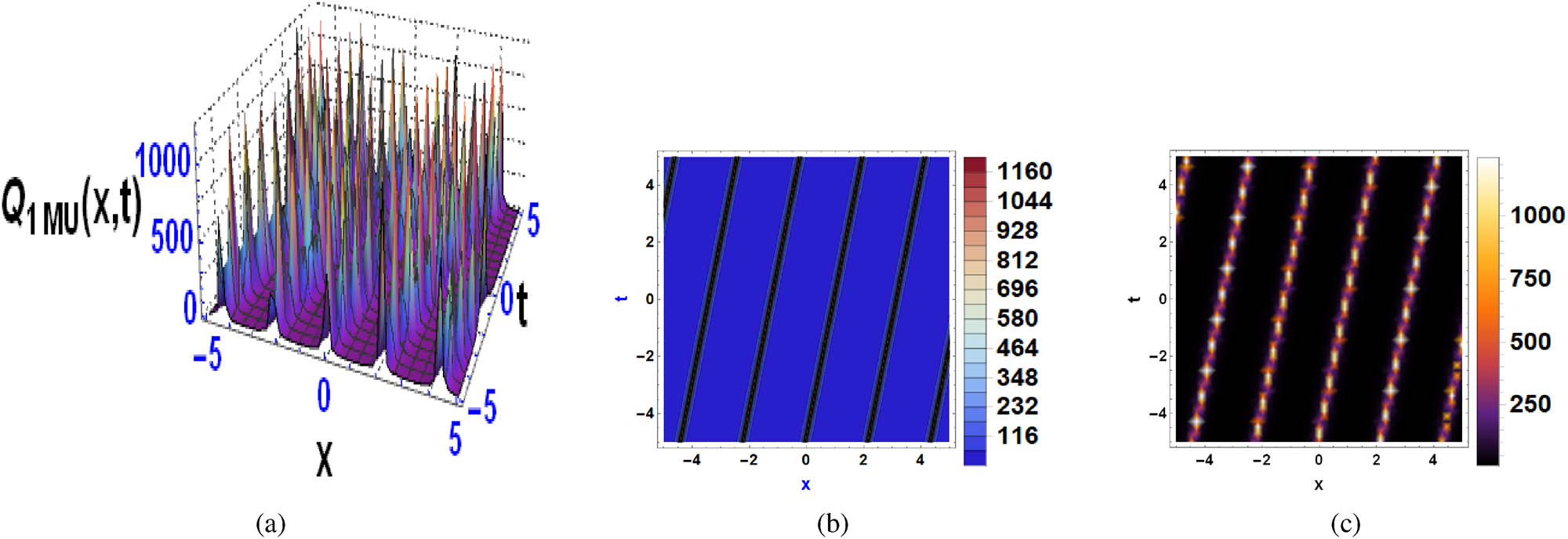
Graphs showing (a) three-dimensional, (b) contour, and (c) density plots of the solution

Graphs showing (a) three-dimensional, (b) contour, and (c) density plots of the solution

Graphs showing (a) three-dimensional, (b) contour, and (c) density plots of the solution

Graphs showing (a) three-dimensional, (b) contour, and (c) density plots of the solution

Graphs showing (a) three-dimensional, (b) contour, and (c) density plots of the solution

Graphs showing (a) three-dimensional, (b) contour, and (c) density plots of the solution

Graphs showing (a) three-dimensional, (b) contour, and (c) density plots of the solution

Graphs showing (a) three-dimensional, (b) contour, and (c) density plots of the solution

Graphs showing (a) three-dimensional, (b) contour, and (c) density plots of the solution

Graphs showing (a) three-dimensional, (b) contour, and (c) density plots of the solution
It is worth noting that multi-wave solutions depict how several interacting primary wave fronts of diverse contents lead to the emergence of distortion and stress profiles. Periodic lump waves illustrate how energy is being sustained within given intervals, thereby showing that the material is subjected to compressive forces for a while before being released. These wave types are crucial in elucidating the ability of elastic rods to store and transmit energy in a cyclical manner, which is a key aspect in the study of wave motion in solids. Furthermore, periodic cross-kink waves show clear uniform regions that are interleaved with narrower regions of apparent distortion, which may suggest buckling or sudden high straining rates in elastic materials under load. Also, we observe that homoclinic breather waves can persist where the oscillations are confined, suggesting that sufficiently long waves with little energy leakage from the rod can be sustained. These aspects help explain the non-trivial content of nonlinear wave propagation in elastic solids. Dark solitons and mixed wave solutions show that there are many ways in which waves interact in Murnaghan’s rods. In this case, dark solitons are areas of depressions or less deformed medium showing some stabilization of the material, whereas mixed wave solutions showcase the fact that elastic rods are capable of having even simultaneous different types of wave motion propagating within them. These facts highlight the intricacy of wave motions in elastic structures and may prove useful for engineering designs as well as for nonlinear wave propagation research in solids.
The physical interpretation of the model parameters helps improve the practical insight into the wave structures obtained. In particular, the parameter
The values utilized in the graphical plots were arbitrarily chosen to ensure visibility, clarity, and variability of the wave structures in question. The values are not experimentally obtained but were selected within physically reasonable ranges to characterize the qualitative character of the exact solutions. The main aim was to exhibit richness of solution space and the effect of parameter variation on wave shape, localization, and interaction. Additional work can include tuning these parameters against actual material properties for application-oriented modeling.
5 Comparison
The solutions achieved in this work, obtained through the Hirota bilinear method, are a major improvement over most of the earlier reported outcomes for DDE as in nonlinear elastic rods. Previous studies have used a wide range of analytical methods such as the sine-Gordon expansion technique [34], extended sinh-Gordon and modified
In contrast, the Hirota bilinear approach is a better structured and integrated procedure that can build up diverse and composite wave structures, including multi-wave interaction, periodic lumps, cross-kink waves, homoclinic breathers, and mixed solitons. The variety of solution types reflects a better insight into the nonlinear processes that govern wave propagation in elastic rods such as those accommodated by Murnaghan’s theory. The capacity of this method to generate topological and non-topological, localized and periodic, and bright and dark soliton solutions places it well in comparison to other analytical methods. In contrast to recent researches involving coupled nonlinear Schrödinger equations that also utilize the Hirota technique to discover new optical soliton structures [48], the present contribution expands its application to mechanical wave systems and thus presents a broader understanding of intricate wave phenomenon in doubly dispersive and nonlinear elastic systems.
6 Conclusion
In this work, we used the Hirota bilinear transformation approach to derive various wave structures, which are solutions of a DDE in an elastic Murnaghan’s rod. Using the Hirota technique, we were able to obtain traveling-wave solutions in the form of periodic lump waves, periodic cross-kink waves, homoclinic breather waves, dark soliton, and mixed waves. In addition, the complex structures and interactions of these wave structures were illustrated in the form of 3D, contour, and density plots. The graphical representations illustrate that the shape of the wave affects the propagation of the wave itself. This is particularly evident in the density plots and wave interaction patterns. As a comment, this method has the ability to describe the deformation of single solitary waves in an elastic perfect material and can suggest how such systems behave physically. To the best of our knowledge, this is the first study in which the Hirota bilinear method is used in the context of doubly dispersive media, and the results derived in this manuscript may apply to both fundamental and practical investigations, especially for engineering designs involving elastic wave propagation.
Future work might involve the examination of the stability, chaos, and perturbation response of the DDE to determine its robustness in the presence of small disturbances. The inclusion of fractional-order derivatives would enable the modeling of memory and hereditary effects in viscoelastic or incompressible elastic materials. Adding stochastic terms could potentially facilitate the inclusion of uncertainties and random disturbance that are generally found in real environments. The other possibility is the generalization of the model to a variable-coefficient problem, which would be more representative of spatial or temporal inhomogeneities of the material. These developments would not only improve theoretical insight into the DDE but also extend its availability to a wider range of physical systems, such as composite materials, biological tissue, and engineered smart materials.
Acknowledgments
The authors wish to thank the anonymous reviewers for their comments. All of their criticisms and suggestions were followed at litteram, resulting in a substantial improvement on the overall quality of this work.
-
Funding information: The authors state no funding involved.
-
Author contributions: Conceptualization, N.A., and J.E.M.D.; methodology, N.A., and; software, B.C., S.M., M.Z.B., N.A., A.R.-L., and J.E.M.-D.; validation, B.C., S.M., M.Z.B., N.A., A.R.-L., and J.E.M.-D.; formal analysis, B.C., S.M., M.Z.B., N.A., and J.E.M.-D.; investigation, N.A., and J.E.M.-D.; resources, B.C., S.M., M.Z.B., N.A., A.R.-L., and J.E.M.-D.; data curation, B.C., S.M., M.Z.B., N.A., A.R.-L., and J.E.M.-D.; writing – original draft preparation, B.C., S.M., M.Z.B., N.A., A.R.-L., and J.E.M.-D.; writing – review and editing, B.C., S.M., M.Z.B., N.A., A.R.-L., and J.E.M.-D.; visualization, B.C.; supervision, N.A., and J.E.M.-D. All authors have accepted responsibility for the entire content of this manuscript and approved its submission.
-
Conflict of interest: Jorge E. Macías-Díaz, who is the co-author of this article, is a current Editorial Board member of Open Physics. This fact did not affect the peer-review process. The authors state no other conflict of interest.
-
Data availability statement: The datasets generated and/or analysed during the current study are available from the corresponding author on reasonable request.
References
[1] Kumar M Exact solutions of systems of nonlinear time-space fractional partial differential equations using an iterative method. J Comput Nonlinear Dyn. 2023;18(10):101003. 10.1115/1.4062910Search in Google Scholar
[2] Dubey VP, Singh J, Alshehri AM, Dubey S, Kumar D. Analysis and fractal dynamics of local fractional partial differential equations occurring in physical sciences. J Comput Nonlinear Dyn. 2023;18(3):031001. 10.1115/1.4056360Search in Google Scholar
[3] Baber MZ, Yasin MW, Xu C, Ahmed N, Iqbal MS. Numerical and analytical study for the stochastic spatial dependent prey-predator dynamical system. J Comput Nonlinear Dyn. 2024;19:10. 10.1115/1.4066038Search in Google Scholar
[4] Akbulut A, Islam SR. Study on the Biswas-Arshed equation with the beta time derivative. Int J Appl Comput Math. 2022;8(4):167. 10.1007/s40819-022-01350-0Search in Google Scholar
[5] Alharbi AR, Almatrafi MB, Lotfy K. Constructions of solitary travelling wave solutions for Ito integro-differential equation arising in plasma physics. Results Phys. 2020;19:103533. 10.1016/j.rinp.2020.103533Search in Google Scholar
[6] Agrawal GP. Nonlinear fiber optics. In: Nonlinear Science at the Dawn of the 21st Century. Berlin, Heidelberg: Springer Berlin Heidelberg; 2000. pp. 195–211. 10.1007/3-540-46629-0_9Search in Google Scholar
[7] Ceesay B, Ahmed N, Baber MZ, Akgul A. Breather, lump, M-shape and other interaction for the Poisson-Nernst-Planck equation in biological membranes. Opt Quantum Electron. 2024;56(5):853. 10.1007/s11082-024-06376-wSearch in Google Scholar
[8] Wang P, Yin F, urRahman M, Khan MA, Baleanu D. Unveiling complexity: Exploring chaos and solitons in modified nonlinear Schrödinger equation. Results Phys. 2024;56:107268. 10.1016/j.rinp.2023.107268Search in Google Scholar
[9] Zahed H, Seadawy AR, Iqbal M. Structure of analytical ion-acoustic solitary wave solutions for the dynamical system of nonlinear wave propagation. Open Phys. 2022;20(1):313–33. 10.1515/phys-2022-0030Search in Google Scholar
[10] Peng X, Zhao YW, Lu X. Data-driven solitons and parameter discovery to the (2+1)-dimensional NLSE in optical fiber communications. Nonlinear Dyn. 2024;112(2):1291–306. 10.1007/s11071-023-09083-5Search in Google Scholar
[11] Barsoum MW, Murugaiah A, Kalidindi SR, Zhen T. Kinking nonlinear elastic solids, nanoindentations, and geology. Phys Rev Lett. 2004;92(25):255508. 10.1103/PhysRevLett.92.255508Search in Google Scholar PubMed
[12] Thomas BB, Betchewe G, Victor KK, Crepin KT. On periodic wave solutions to (1+1)-dimensional nonlinear physical models using the Sine-Cosine method. Acta Appl Math. 2010;110:945–53. 10.1007/s10440-009-9487-4Search in Google Scholar
[13] Nofal TA. Simple equation method for nonlinear partial differential equations and its applications. J Egypt Math Soc. 2016;24(2):204–9. 10.1016/j.joems.2015.05.006Search in Google Scholar
[14] Hussain S, Iqbal MS, Ashraf R, Inc M, Tarar MA. Exploring nonlinear dispersive waves in a disordered medium: an analysis using ϕ6 model expansion method. Opt Quantum Electron. 2023;55(7):651. 10.1007/s11082-023-04851-4Search in Google Scholar
[15] Baber MZ, Seadway AR, Iqbal MS, Ahmed N, Yasin MW, Ahmed MO. Comparative analysis of numerical and newly constructed soliton solutions of stochastic Fisher-type equations in a sufficiently long habitat. Int J Modern Phys B. 2023;37(16):2350155. 10.1142/S0217979223501552Search in Google Scholar
[16] Lu X, Chen SJ. Interaction solutions to nonlinear partial differential equations via Hirota bilinear forms: one-lump-multi-stripe and one-lump-multi-soliton types. Nonlinear Dyn. 2021;103(1):947–77. 10.1007/s11071-020-06068-6Search in Google Scholar
[17] Khan MI, Farooq A, Nisar KS, Shah NA. Unveiling new exact solutions of the unstable nonlinear Schrödinger equation using the improved modified Sardar sub-equation method. Results Phys. 2024;59:107593. 10.1016/j.rinp.2024.107593Search in Google Scholar
[18] Baber MZ, Abbas G, Saeed I, Sulaiman TA, Ahmed N, Ahmad H, et al. Optical solitons for 2D-NLSE in multimode fiber with Kerr nonlinearity and its modulation instability. Modern Phys Lett B. 2024;2450341. 10.1142/S021798492450341XSearch in Google Scholar
[19] Wei L. A function transformation method and exact solutions to a generalized sinh-Gordon equation. Comput Math Appl. 2010;60(11):3003–11. 10.1016/j.camwa.2010.09.062Search in Google Scholar
[20] Batool F, Rezazadeh H, Ali Z, Demirbilek U. Exploring soliton solutions of stochastic Phi-4 equation through extended Sinh-Gordon expansion method. Opt Quantum Electron. 2024;56(5):785. 10.1007/s11082-024-06385-9Search in Google Scholar
[21] Kadkhoda N Application of G′G2-expansion method for solving fractional differential equations. Int J Appl Comput Math. 2017;3:1415–24. 10.1007/s40819-017-0344-2Search in Google Scholar
[22] Ali A, Ahmad J, Javed S. Dynamic investigation to the generalized Yu-Toda-Sasa-Fukuyama equation using Darboux transformation. Opt Quantum Electron. 2024;56(2):166. 10.1007/s11082-023-05562-6Search in Google Scholar
[23] Abdel-Gawad H. I. Field and reverse field solitons in wave-operator nonlinear Schrödinger equation with space-time reverse: Modulation instability. Commun Theoret Phys. 2023;75(6):065005. 10.1088/1572-9494/acce32Search in Google Scholar
[24] Hosseini K, Alizadeh F, Hinçal E, Ilie M, Osman MS. Bilinear Bäcklund transformation, Lax pair, Painlevé integrability, and different wave structures of a 3D generalized KdV equation. Nonlinear Dyn. 2024;112(20):18397–411. 10.1007/s11071-024-09944-7Search in Google Scholar
[25] Kumar M, Jhinga A, Majithia JT. Solutions of time-space fractional partial differential equations using Picard’s iterative method. J Comput Nonlinear Dyn. 2024;19(3):031006. 10.1115/1.4064553Search in Google Scholar
[26] Fafa W, Odibat Z, Shawagfeh N. The homotopy analysis method for solving differential equations With generalized Caputo-type fractional derivatives. J Comput Nonlinear Dyn 2023;18(2):021004. 10.1115/1.4056392Search in Google Scholar
[27] Cattani C, Sulaiman TA, Baskonus HM, Bulut H. Solitons in an inhomogeneous Murnaghan’s rod. Europ Phys J Plus. 2018;133:1–11. 10.1140/epjp/i2018-12085-ySearch in Google Scholar
[28] Samsonov AM. Strain solitons in solids and how to construct them. CRC Press; 2001. 10.1201/9781420026139Search in Google Scholar
[29] Rushchitsky JJ, Cattani C. Similarities and differences between the Murnaghan and Signorini descriptions of the evolution of quadratically nonlinear hyperelastic plane waves. Int Appl Mech. 2006;42:997–1010. 10.1007/s10778-006-0170-4Search in Google Scholar
[30] Silambarasan R, Baskonus HM, Bulut H. Jacobi elliptic function solutions of the double dispersive equation in the Murnaghan’s rod. Europ Phys J Plus. 2019;134:1–22. 10.1140/epjp/i2019-12541-2Search in Google Scholar
[31] Rani M, Ahmed N, Dragomir SS, Mohyud-Din ST, Khan I, Nisar KS. Some newly explored exact solitary wave solutions to nonlinear inhomogeneous Murnaghan’s rod equation of fractional order. J Taibah Univ Sci. 2021;15(1):97–110. 10.1080/16583655.2020.1841472Search in Google Scholar
[32] Dusunceli F, Celik E, Askin M, Bulut H. New exact solutions for the doubly dispersive equation using the improved Bernoulli sub-equation function method. Indian J Phys. 2021;95:309–14. Search in Google Scholar
[33] Alquran M, Al Smadi T Generating new symmetric bi-peakon and singular bi-periodic profile solutions to the generalized doubly dispersive equation. Opt Quantum Electron. 2023;55(8):736. 10.1007/s11082-023-05035-wSearch in Google Scholar
[34] Yel G. New wave patterns to the doubly dispersive equation in nonlinear dynamic elasticity. Pramana. 2020;94(1):79. 10.1007/s12043-020-1941-xSearch in Google Scholar
[35] Ahmed MS, Zaghrout AA, Ahmed HM. Travelling wave solutions for the doubly dispersive equation using improved modified extended tanh-function method. Alexandr Eng J. 2022;61(10):7987–94. 10.1016/j.aej.2022.01.057Search in Google Scholar
[36] Alharthi M. S. Wave solitons to a nonlinear doubly dispersive equation in describing the nonlinear wave propagation via two analytical techniques. Results Phys. 2023;47:106362. 10.1016/j.rinp.2023.106362Search in Google Scholar
[37] Rehman SU, Seadawy AR, Rizvi STR, Ahmed S, Althobaiti S. Investigation of double dispersive waves in nonlinear elastic inhomogeneous Murnaghan’s rod. Modern Phys Lett B. 2022;36(8):2150628. 10.1142/S0217984921506284Search in Google Scholar
[38] Ozisik M, Secer A, Bayram M, Sulaiman TA, Yusuf A Acquiring the solitons of inhomogeneous Murnaghan’s rod using extended Kudryashov method with Bernoulli–Riccati approach. Int J Modern Phys B. 2022;36(30):2250221. 10.1142/S0217979222502216Search in Google Scholar
[39] Ibrahim S, Sulaiman TA, Yusuf A, Ozsahin DU, Baleanu D. Wave propagation to the doubly dispersive equation and the improved Boussinesq equation. Opt Quantum Electron. 2024;56(1):20. 10.1007/s11082-023-05571-5Search in Google Scholar
[40] Younas U, Bilal M, Sulaiman TA, Ren J, Yusuf A. On the exact soliton solutions and different wave structures to the double dispersive equation. Opt Quantum Electron. 2022;54:1–22. 10.1007/s11082-021-03445-2Search in Google Scholar
[41] Abourabia AM, Eldreeny YA. A soliton solution of the DD-equation of the Murnaghan’s rod via the commutative hyper complex analysis. Partial Differ Equ Appl Math. 2022;6:100420. 10.1016/j.padiff.2022.100420Search in Google Scholar
[42] Asjad MI, Faridi WA, Jhangeer A, Ahmad H, Abdel-Khalek S, Alshehri N. Propagation of some new traveling wave patterns of the double dispersive equation. Open Phys. 2022;20(1):130–41. 10.1515/phys-2022-0014Search in Google Scholar
[43] Dusunceli F, Celik E, Askin M, Bulut H New exact solutions for the doubly dispersive equation using the improved Bernoulli sub-equation function method. Indian J Phys. 2021;95:309–14. 10.1007/s12648-020-01707-5Search in Google Scholar
[44] Eremeyev VE, Kolpakov AG. Solitary waves in Murnaghan’s rod: Numerical simulations based on the generalized dispersive model. J Appl Mech Tech Phys. 2012;53(4):565–75. Search in Google Scholar
[45] Eremeyev VE, Movchan AB Movchan NV. Dispersion properties of harmonic waves in a rod with a nonuniform cross section. J Eng Math. 2016;98(1):1–18. Search in Google Scholar
[46] Islam SR Bifurcation analysis and soliton solutions to the doubly dispersive equation in elastic inhomogeneous Murnaghan’s rod. Sci Rep. 2024;14(1):11428. 10.1038/s41598-024-62113-zSearch in Google Scholar PubMed PubMed Central
[47] Khatun MM, Gepreel KA, Akbar MA. Dynamics of solitons of the ß-fractional doubly dispersive model: stability and phase portrait analysis. Indian J Phys. 2025;1–16. 10.1007/s12648-025-03602-3.Search in Google Scholar
[48] Khater M, Wang H, Alfalqi SH, Vokhmintsev A, Owyed S. Insights into acoustic beams in nonlinear, weakly dispersive and dissipative media. Opt Quantum Electron. 2025;57(5):1–18. 10.1007/s11082-025-08220-1Search in Google Scholar
[49] Naz S, Rani A, Ul Hassan QM, Ahmad J, Rehman SU, Shakeel M. Dynamic study of new soliton solutions of time-fractional longitudinal wave equation using an analytical approach. Int J Modern Phys B. 2024;38(31):2450420. 10.1142/S0217979224504204Search in Google Scholar
[50] Alsallami SA, Rizvi ST, Seadawy AR. Study of stochastic-fractional Drinfelad-Sokolov-Wilson equation for M-shaped rational, homoclinic breather, periodic and Kink-Cross rational solutions. Mathematics. 2023;11(6):1504. 10.3390/math11061504Search in Google Scholar
[51] Garcia Guirao JL, Baskonus HM, Kumar A. Regarding new wave patterns of the newly extended nonlinear (2+1)-dimensional Boussinesq equation with fourth order. Mathematics. 2020;8(3):341. 10.3390/math8030341Search in Google Scholar
[52] Ceesay B, Baber MZ, Ahmed N, Akguuul A, Cordero A, Torregrosa JR. Modelling symmetric ion-acoustic wave structures for the BBMPB equation in fluid ions using Hirotaas bilinear technique. Symmetry 2023;15(9):1682. 10.3390/sym15091682Search in Google Scholar
[53] Yang XF, Wei Y Bilinear equation of the nonlinear partial differential equation and its application. J Funct Spaces 2020;2020(1)4912159. 10.1155/2020/4912159Search in Google Scholar
[54] Wazwaz AM. The Hirota’s direct method and the tanh–coth method for multiple-soliton solutions of the Sawada-Kotera-Ito seventh-order equation. Appl Math Comput. 2008;199(1):133–8. 10.1016/j.amc.2007.09.034Search in Google Scholar
[55] Hereman W, Zhuang W. Symbolic computation of solitons via Hirota’s bilinear method. Department of Mathematical and Computer Sciences, Colorado, School of Mines. 1994. Search in Google Scholar
[56] Rizvi ST, Seadawy AR, Nimra, Ahmad A. Study of lump, rogue, multi, M shaped, periodic cross kink, breather lump, kink-cross rational waves and other interactions to the Kraenkel-Manna-Merle system in a saturated ferromagnetic material. Opt Quantum Electron. 2023;55(9):813. 10.1007/s11082-023-04972-wSearch in Google Scholar
[57] Wang M, Tian B, Quuu QX, Zhao XH, Zhang Z, Tian HY. Lump, lumpoff, rogue wave, breather wave and periodic lump solutions for a (3+1)-dimensional generalized Kadomtsev-Petviashvili equation in fluid mechanics and plasma physics. Int J Comput Math. 2020;97(12):2474–86. 10.1080/00207160.2019.1704741Search in Google Scholar
[58] Khan MH, Wazwaz AM. Lump, multi-lump, cross kinky-lump and manifold periodic-soliton solutions for the (2+1)-D Calogero-Bogoyavlenskii-Schiff equation. Heliyon. 2020;6(4):e03701. 10.1016/j.heliyon.2020.e03701Search in Google Scholar PubMed PubMed Central
[59] Zhao Z, Chen Y, Han B. Lump soliton, mixed lump stripe and periodic lump solutions of a (2+1)-dimensional asymmetrical Nizhnik-Novikov-Veselov equation. Modern Phys Lett B. 2017;31(14):1750157. 10.1142/S0217984917501573Search in Google Scholar
[60] Ren B, Lin J, Lou ZM. A new nonlinear equation with lump-soliton, lump-periodic, and lump-periodic-soliton solutions. Complexity. 2019;2019(1):4072754. 10.1155/2019/4072754Search in Google Scholar
[61] Rizvi STR, Seadawy AR, Ashraf MA, Bashir A, Younis M, Baleanu D. Multi-wave, homoclinic breather, M-shaped rational and other solitary wave solutions for coupled-Higgs equation. Europ Phys J Special Topics. 2021;230(18):3519–32. 10.1140/epjs/s11734-021-00270-2Search in Google Scholar
[62] Yel G, Cattani C, Baskonus HM, Gao W. On the complex simulations with dark-bright to the Hirota-Maccari system. J Comput Nonlinear Dyn. 2021;16(6):061005. 10.1115/1.4050677Search in Google Scholar
[63] Ozsahin DU, Ceesay B, Baber MZ, Ahmed N, Raza A, Rafiq M, et al. Multiwaves, breathers, lump and other solutions for the Heimburg model in biomembranes and nerves. Sci Rep. 2024;14(1):10180. 10.1038/s41598-024-60689-0Search in Google Scholar PubMed PubMed Central
[64] Ceesay B, Ahmed N, Macías-Díaz JE. Construction of M-shaped solitons for a modified regularized long-wave equation via Hirota’s bilinear method. Open Phys. 2024;22(1):20240057. 10.1515/phys-2024-0057Search in Google Scholar
[65] Tedjani AH, Seadawy AR, Rizvi ST, Solouma E. Dynamical structure and soliton solutions galore: investigating the range of forms in the perturbed nonlinear Schrödinger dynamical equation. Opt Quantum Electron. 2024;56(5):764. 10.1007/s11082-024-06498-1Search in Google Scholar
[66] Ceesay B, Baber MZ, Ahmed N, Macías S, Macías-Díaz JE, Medina-Guevara MG. Solitonic wave solutions of a Hamiltonian nonlinear atom chain model through the Hirota bilinear transformation method. Open Phys. 2025;23(1):20250150. 10.1515/phys-2025-0150Search in Google Scholar
[67] Rizvi ST, Seadawy AR, Ahmed S. Bell and Kink type, Weierstrass and Jacobi elliptic, multiwave, kinky breather, M-shaped and periodic-kink-cross rational solutions for Einstein’s vacuum field model. Opt Quantum Electron. 2024;56(3):456. 10.1007/s11082-023-06037-4Search in Google Scholar
© 2025 the author(s), published by De Gruyter
This work is licensed under the Creative Commons Attribution 4.0 International License.
Articles in the same Issue
- Research Articles
- Single-step fabrication of Ag2S/poly-2-mercaptoaniline nanoribbon photocathodes for green hydrogen generation from artificial and natural red-sea water
- Abundant new interaction solutions and nonlinear dynamics for the (3+1)-dimensional Hirota–Satsuma–Ito-like equation
- A novel gold and SiO2 material based planar 5-element high HPBW end-fire antenna array for 300 GHz applications
- Explicit exact solutions and bifurcation analysis for the mZK equation with truncated M-fractional derivatives utilizing two reliable methods
- Optical and laser damage resistance: Role of periodic cylindrical surfaces
- Numerical study of flow and heat transfer in the air-side metal foam partially filled channels of panel-type radiator under forced convection
- Water-based hybrid nanofluid flow containing CNT nanoparticles over an extending surface with velocity slips, thermal convective, and zero-mass flux conditions
- Dynamical wave structures for some diffusion--reaction equations with quadratic and quartic nonlinearities
- Solving an isotropic grey matter tumour model via a heat transfer equation
- Study on the penetration protection of a fiber-reinforced composite structure with CNTs/GFP clip STF/3DKevlar
- Influence of Hall current and acoustic pressure on nanostructured DPL thermoelastic plates under ramp heating in a double-temperature model
- Applications of the Belousov–Zhabotinsky reaction–diffusion system: Analytical and numerical approaches
- AC electroosmotic flow of Maxwell fluid in a pH-regulated parallel-plate silica nanochannel
- Interpreting optical effects with relativistic transformations adopting one-way synchronization to conserve simultaneity and space–time continuity
- Modeling and analysis of quantum communication channel in airborne platforms with boundary layer effects
- Theoretical and numerical investigation of a memristor system with a piecewise memductance under fractal–fractional derivatives
- Tuning the structure and electro-optical properties of α-Cr2O3 films by heat treatment/La doping for optoelectronic applications
- High-speed multi-spectral explosion temperature measurement using golden-section accelerated Pearson correlation algorithm
- Dynamic behavior and modulation instability of the generalized coupled fractional nonlinear Helmholtz equation with cubic–quintic term
- Study on the duration of laser-induced air plasma flash near thin film surface
- Exploring the dynamics of fractional-order nonlinear dispersive wave system through homotopy technique
- The mechanism of carbon monoxide fluorescence inside a femtosecond laser-induced plasma
- Numerical solution of a nonconstant coefficient advection diffusion equation in an irregular domain and analyses of numerical dispersion and dissipation
- Numerical examination of the chemically reactive MHD flow of hybrid nanofluids over a two-dimensional stretching surface with the Cattaneo–Christov model and slip conditions
- Impacts of sinusoidal heat flux and embraced heated rectangular cavity on natural convection within a square enclosure partially filled with porous medium and Casson-hybrid nanofluid
- Stability analysis of unsteady ternary nanofluid flow past a stretching/shrinking wedge
- Solitonic wave solutions of a Hamiltonian nonlinear atom chain model through the Hirota bilinear transformation method
- Bilinear form and soltion solutions for (3+1)-dimensional negative-order KdV-CBS equation
- Solitary chirp pulses and soliton control for variable coefficients cubic–quintic nonlinear Schrödinger equation in nonuniform management system
- Influence of decaying heat source and temperature-dependent thermal conductivity on photo-hydro-elasto semiconductor media
- Dissipative disorder optimization in the radiative thin film flow of partially ionized non-Newtonian hybrid nanofluid with second-order slip condition
- Bifurcation, chaotic behavior, and traveling wave solutions for the fractional (4+1)-dimensional Davey–Stewartson–Kadomtsev–Petviashvili model
- New investigation on soliton solutions of two nonlinear PDEs in mathematical physics with a dynamical property: Bifurcation analysis
- Mathematical analysis of nanoparticle type and volume fraction on heat transfer efficiency of nanofluids
- Creation of single-wing Lorenz-like attractors via a ten-ninths-degree term
- Optical soliton solutions, bifurcation analysis, chaotic behaviors of nonlinear Schrödinger equation and modulation instability in optical fiber
- Chaotic dynamics and some solutions for the (n + 1)-dimensional modified Zakharov–Kuznetsov equation in plasma physics
- Fractal formation and chaotic soliton phenomena in nonlinear conformable Heisenberg ferromagnetic spin chain equation
- Single-step fabrication of Mn(iv) oxide-Mn(ii) sulfide/poly-2-mercaptoaniline porous network nanocomposite for pseudo-supercapacitors and charge storage
- Novel constructed dynamical analytical solutions and conserved quantities of the new (2+1)-dimensional KdV model describing acoustic wave propagation
- Tavis–Cummings model in the presence of a deformed field and time-dependent coupling
- Spinning dynamics of stress-dependent viscosity of generalized Cross-nonlinear materials affected by gravitationally swirling disk
- Design and prediction of high optical density photovoltaic polymers using machine learning-DFT studies
- Robust control and preservation of quantum steering, nonlocality, and coherence in open atomic systems
- Coating thickness and process efficiency of reverse roll coating using a magnetized hybrid nanomaterial flow
- Dynamic analysis, circuit realization, and its synchronization of a new chaotic hyperjerk system
- Decoherence of steerability and coherence dynamics induced by nonlinear qubit–cavity interactions
- Finite element analysis of turbulent thermal enhancement in grooved channels with flat- and plus-shaped fins
- Modulational instability and associated ion-acoustic modulated envelope solitons in a quantum plasma having ion beams
- Statistical inference of constant-stress partially accelerated life tests under type II generalized hybrid censored data from Burr III distribution
- On solutions of the Dirac equation for 1D hydrogenic atoms or ions
- Entropy optimization for chemically reactive magnetized unsteady thin film hybrid nanofluid flow on inclined surface subject to nonlinear mixed convection and variable temperature
- Stability analysis, circuit simulation, and color image encryption of a novel four-dimensional hyperchaotic model with hidden and self-excited attractors
- A high-accuracy exponential time integration scheme for the Darcy–Forchheimer Williamson fluid flow with temperature-dependent conductivity
- Novel analysis of fractional regularized long-wave equation in plasma dynamics
- Development of a photoelectrode based on a bismuth(iii) oxyiodide/intercalated iodide-poly(1H-pyrrole) rough spherical nanocomposite for green hydrogen generation
- Investigation of solar radiation effects on the energy performance of the (Al2O3–CuO–Cu)/H2O ternary nanofluidic system through a convectively heated cylinder
- Quantum resources for a system of two atoms interacting with a deformed field in the presence of intensity-dependent coupling
- Studying bifurcations and chaotic dynamics in the generalized hyperelastic-rod wave equation through Hamiltonian mechanics
- A new numerical technique for the solution of time-fractional nonlinear Klein–Gordon equation involving Atangana–Baleanu derivative using cubic B-spline functions
- Interaction solutions of high-order breathers and lumps for a (3+1)-dimensional conformable fractional potential-YTSF-like model
- Hydraulic fracturing radioactive source tracing technology based on hydraulic fracturing tracing mechanics model
- Numerical solution and stability analysis of non-Newtonian hybrid nanofluid flow subject to exponential heat source/sink over a Riga sheet
- Numerical investigation of mixed convection and viscous dissipation in couple stress nanofluid flow: A merged Adomian decomposition method and Mohand transform
- Effectual quintic B-spline functions for solving the time fractional coupled Boussinesq–Burgers equation arising in shallow water waves
- Analysis of MHD hybrid nanofluid flow over cone and wedge with exponential and thermal heat source and activation energy
- Solitons and travelling waves structure for M-fractional Kairat-II equation using three explicit methods
- Impact of nanoparticle shapes on the heat transfer properties of Cu and CuO nanofluids flowing over a stretching surface with slip effects: A computational study
- Computational simulation of heat transfer and nanofluid flow for two-sided lid-driven square cavity under the influence of magnetic field
- Irreversibility analysis of a bioconvective two-phase nanofluid in a Maxwell (non-Newtonian) flow induced by a rotating disk with thermal radiation
- Hydrodynamic and sensitivity analysis of a polymeric calendering process for non-Newtonian fluids with temperature-dependent viscosity
- Exploring the peakon solitons molecules and solitary wave structure to the nonlinear damped Kortewege–de Vries equation through efficient technique
- Modeling and heat transfer analysis of magnetized hybrid micropolar blood-based nanofluid flow in Darcy–Forchheimer porous stenosis narrow arteries
- Activation energy and cross-diffusion effects on 3D rotating nanofluid flow in a Darcy–Forchheimer porous medium with radiation and convective heating
- Insights into chemical reactions occurring in generalized nanomaterials due to spinning surface with melting constraints
- Influence of a magnetic field on double-porosity photo-thermoelastic materials under Lord–Shulman theory
- Soliton-like solutions for a nonlinear doubly dispersive equation in an elastic Murnaghan's rod via Hirota's bilinear method
- Analytical and numerical investigation of exact wave patterns and chaotic dynamics in the extended improved Boussinesq equation
- Nonclassical correlation dynamics of Heisenberg XYZ states with (x, y)-spin--orbit interaction, x-magnetic field, and intrinsic decoherence effects
- Exact traveling wave and soliton solutions for chemotaxis model and (3+1)-dimensional Boiti–Leon–Manna–Pempinelli equation
- Unveiling the transformative role of samarium in ZnO: Exploring structural and optical modifications for advanced functional applications
- On the derivation of solitary wave solutions for the time-fractional Rosenau equation through two analytical techniques
- Analyzing the role of length and radius of MWCNTs in a nanofluid flow influenced by variable thermal conductivity and viscosity considering Marangoni convection
- Advanced mathematical analysis of heat and mass transfer in oscillatory micropolar bio-nanofluid flows via peristaltic waves and electroosmotic effects
- Exact bound state solutions of the radial Schrödinger equation for the Coulomb potential by conformable Nikiforov–Uvarov approach
- Some anisotropic and perfect fluid plane symmetric solutions of Einstein's field equations using killing symmetries
- Nonlinear dynamics of the dissipative ion-acoustic solitary waves in anisotropic rotating magnetoplasmas
- Curves in multiplicative equiaffine plane
- Exact solution of the three-dimensional (3D) Z2 lattice gauge theory
- Propagation properties of Airyprime pulses in relaxing nonlinear media
- Symbolic computation: Analytical solutions and dynamics of a shallow water wave equation in coastal engineering
- Wave propagation in nonlocal piezo-photo-hygrothermoelastic semiconductors subjected to heat and moisture flux
- Comparative reaction dynamics in rotating nanofluid systems: Quartic and cubic kinetics under MHD influence
- Laplace transform technique and probabilistic analysis-based hypothesis testing in medical and engineering applications
- Physical properties of ternary chloro-perovskites KTCl3 (T = Ge, Al) for optoelectronic applications
- Gravitational length stretching: Curvature-induced modulation of quantum probability densities
- The search for the cosmological cold dark matter axion – A new refined narrow mass window and detection scheme
- A comparative study of quantum resources in bipartite Lipkin–Meshkov–Glick model under DM interaction and Zeeman splitting
- PbO-doped K2O–BaO–Al2O3–B2O3–TeO2-glasses: Mechanical and shielding efficacy
- Nanospherical arsenic(iii) oxoiodide/iodide-intercalated poly(N-methylpyrrole) composite synthesis for broad-spectrum optical detection
- Sine power Burr X distribution with estimation and applications in physics and other fields
- Numerical modeling of enhanced reactive oxygen plasma in pulsed laser deposition of metal oxide thin films
- Dynamical analyses and dispersive soliton solutions to the nonlinear fractional model in stratified fluids
- Computation of exact analytical soliton solutions and their dynamics in advanced optical system
- An innovative approximation concerning the diffusion and electrical conductivity tensor at critical altitudes within the F-region of ionospheric plasma at low latitudes
- An analytical investigation to the (3+1)-dimensional Yu–Toda–Sassa–Fukuyama equation with dynamical analysis: Bifurcation
- Swirling-annular-flow-induced instability of a micro shell considering Knudsen number and viscosity effects
- Numerical analysis of non-similar convection flows of a two-phase nanofluid past a semi-infinite vertical plate with thermal radiation
- MgO NPs reinforced PCL/PVC nanocomposite films with enhanced UV shielding and thermal stability for packaging applications
- Optimal conditions for indoor air purification using non-thermal Corona discharge electrostatic precipitator
- Investigation of thermal conductivity and Raman spectra for HfAlB, TaAlB, and WAlB based on first-principles calculations
- Tunable double plasmon-induced transparency based on monolayer patterned graphene metamaterial
- DSC: depth data quality optimization framework for RGBD camouflaged object detection
- A new family of Poisson-exponential distributions with applications to cancer data and glass fiber reliability
- Numerical investigation of couple stress under slip conditions via modified Adomian decomposition method
- Monitoring plateau lake area changes in Yunnan province, southwestern China using medium-resolution remote sensing imagery: applicability of water indices and environmental dependencies
- Heterodyne interferometric fiber-optic gyroscope
- Exact solutions of Einstein’s field equations via homothetic symmetries of non-static plane symmetric spacetime
- A widespread study of discrete entropic model and its distribution along with fluctuations of energy
- Empirical model integration for accurate charge carrier mobility simulation in silicon MOSFETs
- The influence of scattering correction effect based on optical path distribution on CO2 retrieval
- Anisotropic dissociation and spectral response of 1-Bromo-4-chlorobenzene under static directional electric fields
- Role of tungsten oxide (WO3) on thermal and optical properties of smart polymer composites
- Analysis of iterative deblurring: no explicit noise
- 10.1515/phys-2025-0251
- Review Article
- Examination of the gamma radiation shielding properties of different clay and sand materials in the Adrar region
- Erratum
- Erratum to “On Soliton structures in optical fiber communications with Kundu–Mukherjee–Naskar model (Open Physics 2021;19:679–682)”
- Special Issue on Fundamental Physics from Atoms to Cosmos - Part II
- Possible explanation for the neutron lifetime puzzle
- Special Issue on Nanomaterial utilization and structural optimization - Part III
- Numerical investigation on fluid-thermal-electric performance of a thermoelectric-integrated helically coiled tube heat exchanger for coal mine air cooling
- Special Issue on Nonlinear Dynamics and Chaos in Physical Systems
- Analysis of the fractional relativistic isothermal gas sphere with application to neutron stars
- Abundant wave symmetries in the (3+1)-dimensional Chafee–Infante equation through the Hirota bilinear transformation technique
- Successive midpoint method for fractional differential equations with nonlocal kernels: Error analysis, stability, and applications
- Novel exact solitons to the fractional modified mixed-Korteweg--de Vries model with a stability analysis