Tavis–Cummings model in the presence of a deformed field and time-dependent coupling
-
Mariam Algarni


Abstract
In this work, we introduce a model for a two-atom (T–A) system interacting with a field mode initially prepared in a coherent state of a Para Bose–field (P–F). The T–As are initially represented by a Bell state, and we present the quantum framework for the whole system by solving the dynamical equations. We investigate the time-dependent behavior of essential quantum resources relevant to various tasks in quantum optics and information science, including atomic population inversion, T–As entanglement, T–As-P–F entanglement, and the statistical properties of the P–F as they relate to the model parameters. Our analysis reveals how these quantum resources are affected by different parameters in the T–As-P–F model. Finally, we illustrate the evolving interdependencies among these quantum resources within the system.
1 Introduction
The interaction between light and matter is the main focus of quantum optics [1]. The primary and most widely used two models in quantum optics is the Jaynes (Tavis)-Cumming model J–CM (T–CM), which includes one atom and two atoms (T–As) in the presence of field modes [2,3]. The rotating wave approximation and dipole provided an exact solution. The J–CM (T–CM) model’s integrable Hamiltonian was solved to obtain the eigenvalues and eigenvectors of the system under various extensions and quantum effects. The intensity-dependent coupling [4] is one of these extensions. A multi-level atom is another extension, there have been discussions about three-level atoms with constant coupling [5,6,7], four-level atoms [8,9] and five-level atoms in previous literature [10,11,12,13] where nonlinear interactions are considered under different circumstances. A variety of quantum effects are expected within the framework of the J–CM. Examples include the collapse and revival of atomic population inversion, Rabi oscillations, and photon antibunching [14], photon switching [15,16], etc.
Quantum correlations (QCs) are a fundamental feature of quantum systems and serve as an essential tool in the field of quantum information science [17]. Quantum entanglement (QE), one of the most prominent types of QCs, proves valuable for numerous applications, including quantum teleportation [18], quantum key distribution [19], quantum metrology [20], and several others [21,22]. QCs provide precious resources for quantum information tasks. QE had rapid expansion in the last years [23,24], which was also the time when it became an important resource for quantum information processing (QIP). When atomic motion is considered, QIP may have significant applications for the advancement of quantum systems [25]. It has been shown that the von Neumann entropy changes periodically when the time-dependent (t-d) coupling is present. These findings have also been used for the examination of the entanglement that exists between a three-level trapped ion and a laser field [26]. A further extension that may be conducted is to investigate the ways in which the field-mode structure and t-d coupling alter the dynamic characteristics of the cavity field’s Wehrl entropy [27].
In recent decades, numerous researchers have explored extensions and deformations of the bosonic Fock-Heisenberg algebra (HA) to enhance various aspects of quantum field theory, with significant progress made in many areas. Various q-deformations of the simple harmonic oscillator (HO) have been proposed by several authors considering Jackson’s q-calculus [28], leading to the development of novel states associated with q-deformed Lie algebras, including q-coherent, q-squeezed, and q-cat states [29,30,31,32]. Another notable adaptation of the HA is the Wigner algebra, which incorporates the reflection operator
The concept of coherent states (CSs) have been widely used in quantum optics and information during the last several decades. Schrödinger first introduced CSs to describe systems with a Hamiltonian HO that minimizes quantum mechanical uncertainty [45,46]. Actually, two ways are considered for the construction of CSs known as Klauder–Perelomov and Barut–Girardello CSs [42,47,48]. Moreover, several investigations based on the standard creation and annihilation operators in original J–CM are generalized in the context of f-, q-, and λ-deformed operators [49–58]. Moreover, the conventional J–CM with intensity-dependent coupling and interaction of atoms with a field in the context of Holstein–Primakoff SU(2) and SU(1,1) CSs have been examined [59–61]. Some further extensions have been proposed and studied, including transitions between two or more photons [62] and Jaynes–Cummings–Hubbard model [63,64]. Based on the above consideration, in the present we develop the model of T–As interacting with a quantum field initially prepared in a CS of Para Bose–field (P–F). We examine the dynamic behavior of essential quantum resources relevant to various tasks in quantum optics and information. This includes examining atomic population inversion, T–As entanglement, T–As-P–F entanglement, and the statistical properties of P–F, all in relation to the parameters of the quantum model.
The rest of the article is structured as follows: Section 2 provides a description of the quantum system and outlines its dynamics. In Section 3, we discuss the numerical results alongside the measures of quantumness. Finally, our conclusion is summarized in Section 4.
2 Quantum model
This section represents the Hamiltonian of the interaction of one-mode P–F with T–As of an upper (lower) state
where
where
where
The t-d state of the T–As-P–F system at any time
Next we proceed to solve the system’s equation of motion
with initial system state
where
By substituting the t-d state of the system into the motion equation and using the initial conditions, the functions
with
and
The CSs corresponding to the P–F are introduced as [65]
where
The reduced density matrices of subsystems are obtained from the T–As-P–F density matrix,
3 Quantum measures and their dynamical behavior
This section displays different measures for quantumness with their dynamical behavior discussion through the effect of t-d coupling (
3.1 Atomic inversion
We begin by defining the population inversion for the T–As in terms of the functions
In the case where the two atoms are identically coupled, we have
The population inversion,
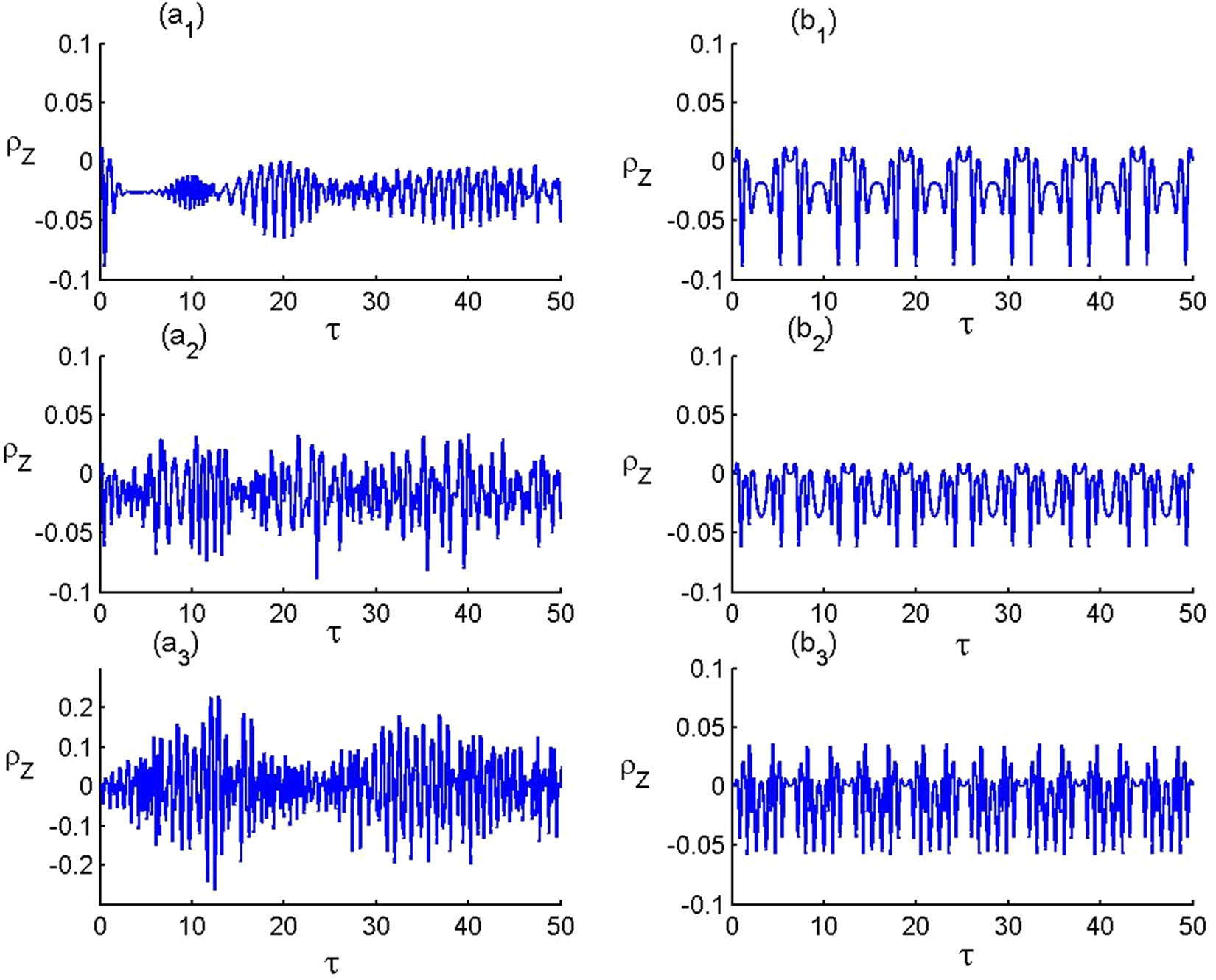
Time evolution of
3.2 T–As-P–F entanglement
To analyze the dynamics of the T–As-P–F entanglement, the Neumann entropy of the subsystems, T–A or P–F, is considered as a measure
Here
where
In Figure 2, we illustrate the dynamic behavior of quantum entropy in relation to the parameter values of the physical model, using the same parameter settings as in Figure 1. The figure highlights significant physical scenarios based on the values of
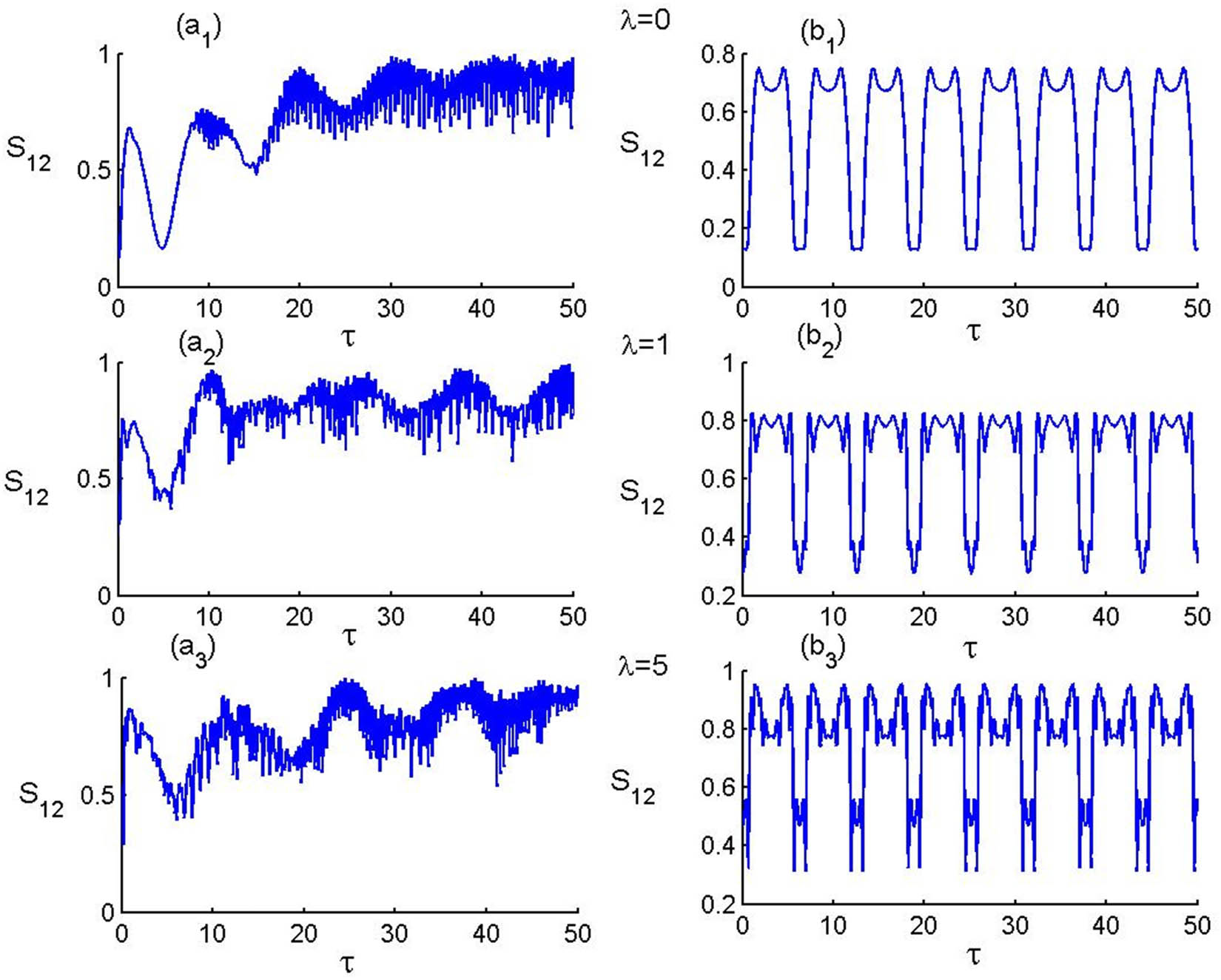
Time evolution of T–As-P–F entanglement in the presence of P–F with
3.3 T–As entanglement
To analyze the nonlocal correlation between the T–As, we utilize the concurrence that is given by [66]
where
Here
Figure 3 shows the time variation of concurrence with regard to the values of the T–As-P–F parameters. In general, it is evident that
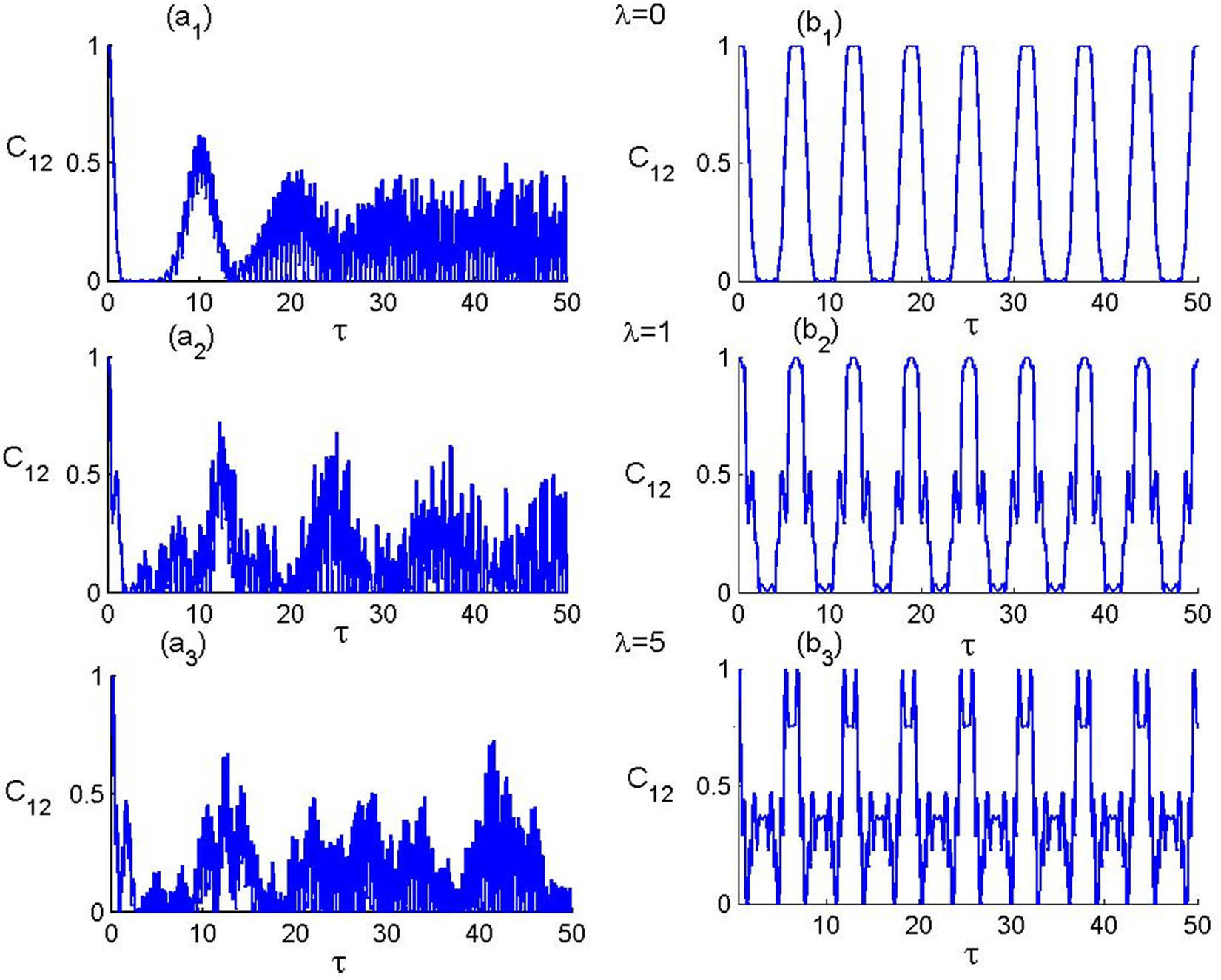
Time evolution of T–As entanglement in the presence of P–F with
3.4 Statistical properties of the P–F
Now, we analyze the distribution of P–F photons using the Mandel parameter that is defined by [67,68]
The P–F exhibits the Poissonian statistics for
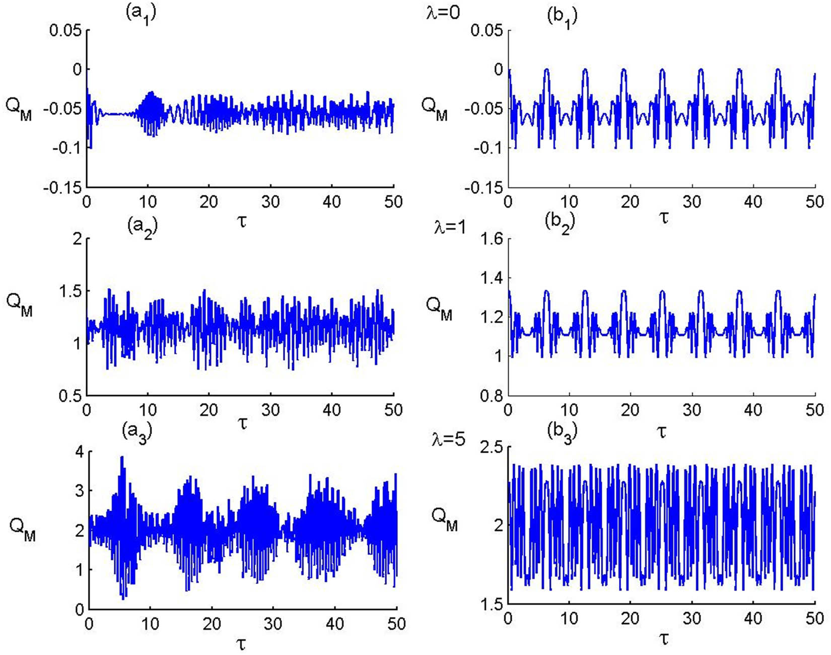
The Mandel parameter for the P–F with
4 Conclusion
In this article, we have developed a model of T–As system that interacts with a field mode initially defined in a CS of P–F. We have considered that the T–As are initially described by a Bell state and display the quantum model of the whole system with the solution of the dynamics equation in the absence and presence of t-d coupling effect. We have examined the t-d behavior of essential quantum resources relevant to various tasks in quantum optics and information science, including atomic population inversion, T–As entanglement, T–As-P–F entanglement, and the statistical properties of the P–F as they relate to the model parameters. In this context, our analysis revealed how these quantum resources are affected by different parameters in the T–As-P–F model. Finally, we have illustrated the evolving interdependencies among these quantum resources within the quantum system.
-
Funding information: Princess Nourah bint Abdulrahman University Researchers Supporting Project number (PNURSP2025R225), Princess Nourah bint Abdulrahman University, Riyadh, Saudi Arabia.
-
Author contributions: All authors have accepted responsibility for the entire content of this manuscript and approved its submission.
-
Conflict of interest: The authors state no conflict of interest.
-
Data availability statement: All data generated or analyzed during this study are included in this published article.
References
[1] Jaynes ET, Cummings FW. Comparison of quantum and semiclassical radiation theories with applications to the beam maser. Proc IEEE. 1963;51:89.10.1109/PROC.1963.1664Search in Google Scholar
[2] Tavis M, Cummings FW. Exact solution for an N-molecule-radiation-field hamiltonian. Phys Rev. 1968;170:379.10.1103/PhysRev.170.379Search in Google Scholar
[3] Cummings FW. Stimulated emission of radiation in a single mode. Phys Rev A. 1965;140:A1051.10.1103/PhysRev.140.A1051Search in Google Scholar
[4] Chang Z. Generalized Jaynes-Cummings model with an intensity-dependent coupling interacting with a quantum group-theoretic coherent state. Phys Rev A. 1993;47:5017–23.10.1103/PhysRevA.47.5017Search in Google Scholar PubMed
[5] Yoo HI, Eberly JH. Dynamical theory of an atom with two or three levels interacting with quantized cavity fields. Phys Rep. 1985;118:239.10.1016/0370-1573(85)90015-8Search in Google Scholar
[6] Tavassoly MK, Yadollahi F. Dynamics of states in the nonlinear interaction regime between a three-level atom and generalized coherent states and their non-classical features. Int J Mod Phys B. 2012;26:1250027.10.1142/S0217979212500270Search in Google Scholar
[7] Fahgihi MJ, Tavassoly MK. Dynamics of entropy and nonclassical properties of the state of a Λ-type three-level atom interacting with a single-mode cavity field with intensity-dependent coupling in a Kerr medium. J Phys B: Mol Opt Phys. 2012;45:035502.10.1088/0953-4075/45/3/035502Search in Google Scholar
[8] Xu W, Gao JY. Absorption mechanism in a four-level system. Phys Rev A. 2003;67:033816–22.10.1103/PhysRevA.67.033816Search in Google Scholar
[9] Abdel-Wahab NH, Thabet L. Dynamics of N-configuration four-level atom interacting with one-mode cavity field. Eur Phys J Plus. 2014;129:1–10.10.1140/epjp/i2014-14144-9Search in Google Scholar
[10] Bhattacharyya D, Ray B, Ghosh PN. Theoretical study of electromagnetically induced transparency in a five-level atom and application to Doppler-broadened and Dopplerfree Rb atoms. J Phys B: At Mol Opt Phys. 2007;40:4061–70.10.1088/0953-4075/40/20/008Search in Google Scholar
[11] Nawaz SM, Tarak ND, Kanhaiya P. Microwave assisted transparency in M-system. J Phys B: At Mol Opt Phys. 2017;50:195502.10.1088/1361-6455/aa8a35Search in Google Scholar
[12] Amanjot K, Paramjit K. Dressed state analysis of electromagnetically induced transparency in a five-level X-type atomic system with wavelength mismatching effects. Phys Scr. 2018;93:115101–18.10.1088/1402-4896/aadec9Search in Google Scholar
[13] Li J, Ren-Gang W. Amplitude and phase-controlled absorption and dispersion of coherently driven five-level atom in double-band photonic crystal. Chin Phys B. 2019;28(2):024206–12.10.1088/1674-1056/28/2/024206Search in Google Scholar
[14] Ben1 L, Jing-Biao C. Photon antibunching. Rev Mod Phys. 1982;54:1061.10.1103/RevModPhys.54.1061Search in Google Scholar
[15] Harris SE, Yamamoto Y. Photon switching by quantum interference. Phys Rev Lett. 1998;81:3611–4.10.1103/PhysRevLett.81.3611Search in Google Scholar
[16] Yan M, Edward G, Zhu Y. Observation and absorptive photon switching by quantum interference. Phys Rev A. 2001;64:041801–4.10.1103/PhysRevA.64.041801Search in Google Scholar
[17] Bell JS. On the Einstein Podolsky Rosen paradox. Phys Phys Fiz. 1964;1(3):195.10.1103/PhysicsPhysiqueFizika.1.195Search in Google Scholar
[18] Bennett CH, Brassard G, Crépeau C, Jozsa R, Peres A, Wootters WK. Teleporting an unknown quantum state via dual classical and Einstein-Podolsky-Rosen channels. Phys Rev Lett. 1993;70(13):1895.10.1103/PhysRevLett.70.1895Search in Google Scholar PubMed
[19] Ekert AK. Quantum cryptography based on Bell’s theorem. Phys Rev Lett. 1991;67(6):661.10.1103/PhysRevLett.67.661Search in Google Scholar PubMed
[20] Maccone L. Intuitive reason for the usefulness of entanglement in quantum metrology. Phys Rev A. 2013;88(4):042109.10.1103/PhysRevA.88.042109Search in Google Scholar
[21] Horodecki R, Horodecki P, Horodecki M, Horodecki K. Quantum entanglement. Rev Mod Phys. 2009;81(2):865–942.10.1103/RevModPhys.81.865Search in Google Scholar
[22] Adesso G, Bromley TR, Cianciaruso M. Measures and applications of quantum correlations. J Phys A. 2016;49(47):473001.10.1088/1751-8113/49/47/473001Search in Google Scholar
[23] Brody J. Quantum entanglement. Cambridge, MA: The MIT Press Essential Knowledge series, Paperback–Illustrated; 2020.Search in Google Scholar
[24] Vedral V. Quantum entanglement. Nat Phys. 2014;10:256–8.10.1038/nphys2904Search in Google Scholar
[25] Gingrich RM, Christoph A. Quantum entanglement of moving bodies. Phys Rev Lett. 2002;89:270402.10.1103/PhysRevLett.89.270402Search in Google Scholar PubMed
[26] Abdel-Aty M, Wahiddin MR, Abdalla MS, Obada AS. Entanglement of a three-level trapped atom in the presence of another three-level trapped atom. Opt Commun. 2006;265:551–8.10.1016/j.optcom.2006.03.063Search in Google Scholar
[27] Abdel-Khalek S, Obada A-SF. The atomic Wehrl entropy of a V-type three-level atom interacting with two-mode squeezed vacuum state. J Russ Laser Res. 2009;30:146–56.10.1007/s10946-009-9066-1Search in Google Scholar
[28] Arik M, Coon DD. Hilbert spaces of analytic functions and generalized coherent states. J Math Phys. 1976;17:524.10.1063/1.522937Search in Google Scholar
[29] Fakhri H, Hashemi A. Nonclassical properties of the q-coherent and q-cat states of the Biedenharn–Macfarlane q oscillator with q > 1. Phys Rev A. 2016;93:013802.10.1103/PhysRevA.93.013802Search in Google Scholar
[30] Fakhri H, Sayyah-Fard M. Nonclassical properties of the Arik-Coon q−1-oscillator coherent states on the noncommutative complex plane Cq. Int J Geom Meth Mod Phys. 2017;14:1750165.Search in Google Scholar
[31] Fakhri H, Sayyah-Fard M. q-coherent states associated with the noncommutative complex plane C2 q for the Biedenharn–Macfarlane q-oscillator. Ann Phys. 2017;387:14.10.1142/S0219887817501651Search in Google Scholar
[32] Fakhri H, Sayyah-Fard M. Noncommutative photon-added squeezed vacuum states. Mod Phys Lett A. 2020;35:2050167.10.1142/S0217732320501679Search in Google Scholar
[33] Plyushchay MS. Deformed Heisenberg algebra with reflection. Nucl Phys B. 1997;491:619.10.1016/S0550-3213(97)00065-5Search in Google Scholar
[34] Green HS. A generalized method of field quantization. Phys Rev. 1953;90:270.10.1103/PhysRev.90.270Search in Google Scholar
[35] Ohnuki Y, Kamefuchi S. Quantum field theory and parastatistics. Tokyo: University Press of Tokyo; 1982.10.1007/978-3-642-68622-1Search in Google Scholar
[36] Polychronakos AP. Exchange operator formalism for integrable systems of particles. Phys Rev Lett. 1992;69:703.10.1103/PhysRevLett.69.703Search in Google Scholar PubMed
[37] Brink L, Hansson TH, Konstein S, Vasiliev MA. The Calogero model-anyonic representation, fermionic extension and supersymmetry. Nucl Phys B. 1993;401:591.10.1016/0550-3213(93)90315-GSearch in Google Scholar
[38] Mojaveri B, Dehghani A, Jafarzadeh R. Bahrbeig, Excitation on the para-Bose states: Nonclassical properties. Euro Phys J Plus. 2018;133:346.10.1140/epjp/i2018-12163-2Search in Google Scholar
[39] Dehghani A, Mojaveri B, Bahrbeig RJ, Nosrati F, Franco RL. Entanglement transfer in a noisy cavity network with parity-deformed fields. J Opt Soc Am B. 2019;36:1858.10.1364/JOSAB.36.001858Search in Google Scholar
[40] Mojaveri B, Dehghani A, Ahmadi Z. A quantum correlated heat engine based on the parity-deformed Jaynes–Cummings model: Achieving the classical Carnot efficiency by a local classical field. Phys Scr. 2021;96:115102.10.1088/1402-4896/ac1638Search in Google Scholar
[41] Perelomov AM. Generalized coherent states and some of their applications. Sov Phys Usp. 1977;20:703.10.1070/PU1977v020n09ABEH005459Search in Google Scholar
[42] Perelomov AM. Generalized coherent states and their applications. Berlin: Springer; 1986.10.1007/978-3-642-61629-7Search in Google Scholar
[43] Alderete CH, Vergara LV, Rodriguez-Lara BM. Nonclassical and semiclassical para-Bose states. Phys Rev A. 2017;95:043835.10.1103/PhysRevA.95.043835Search in Google Scholar
[44] Huerta Alderete C, Rodriguez-Lara BM. Simulating para-Fermi oscillators. Sci Rep. 2018;8:11572.10.1038/s41598-018-29771-2Search in Google Scholar PubMed PubMed Central
[45] Shrödinger E. The constant crossover of micro-to macro-mechanics. Naturwissenschaftler. 1926;14:664.Search in Google Scholar
[46] Glauber RJ. Coherent and incoherent states of the radiation field. Phys Rev. 1963;131:2766–88.10.1103/PhysRev.131.2766Search in Google Scholar
[47] Ali ST, Antoine JP, Gazeau JP. Coherent states, wavelets and their generalizations. Berlin: Springer; 2000.10.1007/978-1-4612-1258-4Search in Google Scholar
[48] Man’ko VI, Marmo G, Sudarshan ECG, Zaccaria F. f-Oscillators and nonlinear coherent states. Phys Scr. 1997;55:528.10.1088/0031-8949/55/5/004Search in Google Scholar
[49] Dehghani A, Mojaveri B, Shirin S, Amiri Faseghandis, S. Parity deformed Jaynes-Cummings Model: “Robust maximally entangled states. Sci Rep. 2016;6:38069.10.1038/srep38069Search in Google Scholar PubMed PubMed Central
[50] de los Santos-Sanchez O, Recamier J. f-deformed Jaynes–Cummings model and its nonlinear coherent states. J Phys B. 2012;45:015502.10.1088/0953-4075/45/1/015502Search in Google Scholar
[51] Cordero S, Nahmad-Achar E, Castaños O, López-Peña R. A general system of n levels interacting with electromagnetic modes. Phys Scr. 2017;92:044004.10.1088/1402-4896/aa6363Search in Google Scholar
[52] Cordero S, Castaños O, López-Peña R, Nahmad-Achar E. Variational study of λ and N atomic configurations interacting with an electromagnetic field of two modes. Phys Rev A. 2016;94:013802.10.1103/PhysRevA.94.013802Search in Google Scholar
[53] Castaños O, Cordero S, Nahmad-Achar E, López-Peña R. Coupling n-level atoms with l-modes of quantised light in a resonator. J Phys: Conf Ser. 2016;698(1):012006. IOP Publishing.10.1088/1742-6596/698/1/012006Search in Google Scholar
[54] Cordero S, Nahmad-Achar E, López-Peña R, Castaños O. Polychromatic phase diagram for n-level atoms interacting with ℓ modes of an electromagnetic field. Phys Rev A. 2015;92:053843.10.1103/PhysRevA.92.053843Search in Google Scholar
[55] Medina-Armendariz MA, Quezada LF, Sun GH, Dong SH. Exploring entanglement dynamics in an optomechanical cavity with a type-V qutrit and quantized two-mode field. Phys A: Stat Mech Appl. 2024;635:129514.10.2139/ssrn.4619729Search in Google Scholar
[56] Quezada LF, Zhang GQ, Martín-Ruiz A, Dong. SH. Exploring quantum critical phenomena in a nonlinear Dicke model through algebraic deformation. Results Phys. 2023;55:107157.10.1016/j.rinp.2023.107157Search in Google Scholar
[57] Fakhri H, Mirzaei S, Sayyah-Fard M. Two-photon Jaynes–Cummings model: a two-level atom interacting with the para-Bose field. Quantum Inf Process. 2021;23:398.10.1007/s11128-021-03338-zSearch in Google Scholar
[58] Mojaveri B, Dehghani A, Ahmadi Z, Amiri Faseghandis S. Interaction of a para-Bose state with two two-level atoms: control of dissipation by a local classical field. Eur Phys J Plus. 2020;135:1–25.10.1140/epjp/s13360-020-00236-8Search in Google Scholar
[59] Buzek V. Jaynes–Cummings model with intensity-dependent coupling interacting with Holstein–Primak of SU(1, 1) coherent state. Phys Rev A. 1989;39:3196.10.1103/PhysRevA.39.3196Search in Google Scholar
[60] Buzek V. SU(1,1) squeezing of SU(1,1) generalized coherent states. J Mod Opt. 1990;37:303.10.1080/09500349014550371Search in Google Scholar
[61] Gerry CC, Welc RF. Dynamics of a two-mode two-photon Jaynes–Cummings model interacting with correlated SU(1, 1) coherent states. J Opt Soc Am B. 1992;9:290.10.1364/JOSAB.9.000290Search in Google Scholar
[62] Abdel-Khalek S, Berrada K, Eleuch H, Abel-Aty M. Dynamics of Wehrl entropy of a degenerate two-photon process with a nonlinear medium. Opt Quantum Electron. 2011;42:887–97.10.1007/s11082-011-9498-zSearch in Google Scholar
[63] Li C, Zhang XZ, Song Z. Equivalent spin-orbit interaction in the two-polariton Jaynes–Cummings–Hubbard model. Sci Rep. 2015;5:11945.10.1038/srep11945Search in Google Scholar PubMed PubMed Central
[64] Prasad SB, Martin AM. Effective three-body interactions in Jaynes–Cummings–Hubbard systems. Sci Rep. 2018;8:16253.10.1038/s41598-018-33907-9Search in Google Scholar PubMed PubMed Central
[65] Fakhri H, Sayyah‑Fard M. The Jaynes–Cummings model of a two-level atom in a single-mode para-Bose cavity field. Sci Reports. 2021;11:22861.10.1038/s41598-021-02150-0Search in Google Scholar PubMed PubMed Central
[66] Wootters WK. Entanglement of formation and concurrence. Quantum Inf Comput. 2001;1:27.10.26421/QIC1.1-3Search in Google Scholar
[67] Singh S. Field statistics in some generalized Jaynes-Cummings models. Phys Rev A. 1982;25:3206.10.1103/PhysRevA.25.3206Search in Google Scholar
[68] Mandel L, Wolf E. Optical coherent and quantum optics. Cambridge: Cambridge University Press; 1955.Search in Google Scholar
© 2025 the author(s), published by De Gruyter
This work is licensed under the Creative Commons Attribution 4.0 International License.
Articles in the same Issue
- Research Articles
- Single-step fabrication of Ag2S/poly-2-mercaptoaniline nanoribbon photocathodes for green hydrogen generation from artificial and natural red-sea water
- Abundant new interaction solutions and nonlinear dynamics for the (3+1)-dimensional Hirota–Satsuma–Ito-like equation
- A novel gold and SiO2 material based planar 5-element high HPBW end-fire antenna array for 300 GHz applications
- Explicit exact solutions and bifurcation analysis for the mZK equation with truncated M-fractional derivatives utilizing two reliable methods
- Optical and laser damage resistance: Role of periodic cylindrical surfaces
- Numerical study of flow and heat transfer in the air-side metal foam partially filled channels of panel-type radiator under forced convection
- Water-based hybrid nanofluid flow containing CNT nanoparticles over an extending surface with velocity slips, thermal convective, and zero-mass flux conditions
- Dynamical wave structures for some diffusion--reaction equations with quadratic and quartic nonlinearities
- Solving an isotropic grey matter tumour model via a heat transfer equation
- Study on the penetration protection of a fiber-reinforced composite structure with CNTs/GFP clip STF/3DKevlar
- Influence of Hall current and acoustic pressure on nanostructured DPL thermoelastic plates under ramp heating in a double-temperature model
- Applications of the Belousov–Zhabotinsky reaction–diffusion system: Analytical and numerical approaches
- AC electroosmotic flow of Maxwell fluid in a pH-regulated parallel-plate silica nanochannel
- Interpreting optical effects with relativistic transformations adopting one-way synchronization to conserve simultaneity and space–time continuity
- Modeling and analysis of quantum communication channel in airborne platforms with boundary layer effects
- Theoretical and numerical investigation of a memristor system with a piecewise memductance under fractal–fractional derivatives
- Tuning the structure and electro-optical properties of α-Cr2O3 films by heat treatment/La doping for optoelectronic applications
- High-speed multi-spectral explosion temperature measurement using golden-section accelerated Pearson correlation algorithm
- Dynamic behavior and modulation instability of the generalized coupled fractional nonlinear Helmholtz equation with cubic–quintic term
- Study on the duration of laser-induced air plasma flash near thin film surface
- Exploring the dynamics of fractional-order nonlinear dispersive wave system through homotopy technique
- The mechanism of carbon monoxide fluorescence inside a femtosecond laser-induced plasma
- Numerical solution of a nonconstant coefficient advection diffusion equation in an irregular domain and analyses of numerical dispersion and dissipation
- Numerical examination of the chemically reactive MHD flow of hybrid nanofluids over a two-dimensional stretching surface with the Cattaneo–Christov model and slip conditions
- Impacts of sinusoidal heat flux and embraced heated rectangular cavity on natural convection within a square enclosure partially filled with porous medium and Casson-hybrid nanofluid
- Stability analysis of unsteady ternary nanofluid flow past a stretching/shrinking wedge
- Solitonic wave solutions of a Hamiltonian nonlinear atom chain model through the Hirota bilinear transformation method
- Bilinear form and soltion solutions for (3+1)-dimensional negative-order KdV-CBS equation
- Solitary chirp pulses and soliton control for variable coefficients cubic–quintic nonlinear Schrödinger equation in nonuniform management system
- Influence of decaying heat source and temperature-dependent thermal conductivity on photo-hydro-elasto semiconductor media
- Dissipative disorder optimization in the radiative thin film flow of partially ionized non-Newtonian hybrid nanofluid with second-order slip condition
- Bifurcation, chaotic behavior, and traveling wave solutions for the fractional (4+1)-dimensional Davey–Stewartson–Kadomtsev–Petviashvili model
- New investigation on soliton solutions of two nonlinear PDEs in mathematical physics with a dynamical property: Bifurcation analysis
- Mathematical analysis of nanoparticle type and volume fraction on heat transfer efficiency of nanofluids
- Creation of single-wing Lorenz-like attractors via a ten-ninths-degree term
- Optical soliton solutions, bifurcation analysis, chaotic behaviors of nonlinear Schrödinger equation and modulation instability in optical fiber
- Chaotic dynamics and some solutions for the (n + 1)-dimensional modified Zakharov–Kuznetsov equation in plasma physics
- Fractal formation and chaotic soliton phenomena in nonlinear conformable Heisenberg ferromagnetic spin chain equation
- Single-step fabrication of Mn(iv) oxide-Mn(ii) sulfide/poly-2-mercaptoaniline porous network nanocomposite for pseudo-supercapacitors and charge storage
- Novel constructed dynamical analytical solutions and conserved quantities of the new (2+1)-dimensional KdV model describing acoustic wave propagation
- Tavis–Cummings model in the presence of a deformed field and time-dependent coupling
- Spinning dynamics of stress-dependent viscosity of generalized Cross-nonlinear materials affected by gravitationally swirling disk
- Design and prediction of high optical density photovoltaic polymers using machine learning-DFT studies
- Robust control and preservation of quantum steering, nonlocality, and coherence in open atomic systems
- Coating thickness and process efficiency of reverse roll coating using a magnetized hybrid nanomaterial flow
- Dynamic analysis, circuit realization, and its synchronization of a new chaotic hyperjerk system
- Decoherence of steerability and coherence dynamics induced by nonlinear qubit–cavity interactions
- Finite element analysis of turbulent thermal enhancement in grooved channels with flat- and plus-shaped fins
- Modulational instability and associated ion-acoustic modulated envelope solitons in a quantum plasma having ion beams
- Statistical inference of constant-stress partially accelerated life tests under type II generalized hybrid censored data from Burr III distribution
- On solutions of the Dirac equation for 1D hydrogenic atoms or ions
- Entropy optimization for chemically reactive magnetized unsteady thin film hybrid nanofluid flow on inclined surface subject to nonlinear mixed convection and variable temperature
- Stability analysis, circuit simulation, and color image encryption of a novel four-dimensional hyperchaotic model with hidden and self-excited attractors
- A high-accuracy exponential time integration scheme for the Darcy–Forchheimer Williamson fluid flow with temperature-dependent conductivity
- Novel analysis of fractional regularized long-wave equation in plasma dynamics
- Development of a photoelectrode based on a bismuth(iii) oxyiodide/intercalated iodide-poly(1H-pyrrole) rough spherical nanocomposite for green hydrogen generation
- Investigation of solar radiation effects on the energy performance of the (Al2O3–CuO–Cu)/H2O ternary nanofluidic system through a convectively heated cylinder
- Quantum resources for a system of two atoms interacting with a deformed field in the presence of intensity-dependent coupling
- Studying bifurcations and chaotic dynamics in the generalized hyperelastic-rod wave equation through Hamiltonian mechanics
- A new numerical technique for the solution of time-fractional nonlinear Klein–Gordon equation involving Atangana–Baleanu derivative using cubic B-spline functions
- Interaction solutions of high-order breathers and lumps for a (3+1)-dimensional conformable fractional potential-YTSF-like model
- Hydraulic fracturing radioactive source tracing technology based on hydraulic fracturing tracing mechanics model
- Numerical solution and stability analysis of non-Newtonian hybrid nanofluid flow subject to exponential heat source/sink over a Riga sheet
- Numerical investigation of mixed convection and viscous dissipation in couple stress nanofluid flow: A merged Adomian decomposition method and Mohand transform
- Effectual quintic B-spline functions for solving the time fractional coupled Boussinesq–Burgers equation arising in shallow water waves
- Analysis of MHD hybrid nanofluid flow over cone and wedge with exponential and thermal heat source and activation energy
- Solitons and travelling waves structure for M-fractional Kairat-II equation using three explicit methods
- Impact of nanoparticle shapes on the heat transfer properties of Cu and CuO nanofluids flowing over a stretching surface with slip effects: A computational study
- Computational simulation of heat transfer and nanofluid flow for two-sided lid-driven square cavity under the influence of magnetic field
- Irreversibility analysis of a bioconvective two-phase nanofluid in a Maxwell (non-Newtonian) flow induced by a rotating disk with thermal radiation
- Hydrodynamic and sensitivity analysis of a polymeric calendering process for non-Newtonian fluids with temperature-dependent viscosity
- Exploring the peakon solitons molecules and solitary wave structure to the nonlinear damped Kortewege–de Vries equation through efficient technique
- Modeling and heat transfer analysis of magnetized hybrid micropolar blood-based nanofluid flow in Darcy–Forchheimer porous stenosis narrow arteries
- Activation energy and cross-diffusion effects on 3D rotating nanofluid flow in a Darcy–Forchheimer porous medium with radiation and convective heating
- Insights into chemical reactions occurring in generalized nanomaterials due to spinning surface with melting constraints
- Influence of a magnetic field on double-porosity photo-thermoelastic materials under Lord–Shulman theory
- Soliton-like solutions for a nonlinear doubly dispersive equation in an elastic Murnaghan's rod via Hirota's bilinear method
- Analytical and numerical investigation of exact wave patterns and chaotic dynamics in the extended improved Boussinesq equation
- Nonclassical correlation dynamics of Heisenberg XYZ states with (x, y)-spin--orbit interaction, x-magnetic field, and intrinsic decoherence effects
- Exact traveling wave and soliton solutions for chemotaxis model and (3+1)-dimensional Boiti–Leon–Manna–Pempinelli equation
- Unveiling the transformative role of samarium in ZnO: Exploring structural and optical modifications for advanced functional applications
- On the derivation of solitary wave solutions for the time-fractional Rosenau equation through two analytical techniques
- Analyzing the role of length and radius of MWCNTs in a nanofluid flow influenced by variable thermal conductivity and viscosity considering Marangoni convection
- Advanced mathematical analysis of heat and mass transfer in oscillatory micropolar bio-nanofluid flows via peristaltic waves and electroosmotic effects
- Exact bound state solutions of the radial Schrödinger equation for the Coulomb potential by conformable Nikiforov–Uvarov approach
- Some anisotropic and perfect fluid plane symmetric solutions of Einstein's field equations using killing symmetries
- Nonlinear dynamics of the dissipative ion-acoustic solitary waves in anisotropic rotating magnetoplasmas
- Curves in multiplicative equiaffine plane
- Exact solution of the three-dimensional (3D) Z2 lattice gauge theory
- Propagation properties of Airyprime pulses in relaxing nonlinear media
- Symbolic computation: Analytical solutions and dynamics of a shallow water wave equation in coastal engineering
- Wave propagation in nonlocal piezo-photo-hygrothermoelastic semiconductors subjected to heat and moisture flux
- Comparative reaction dynamics in rotating nanofluid systems: Quartic and cubic kinetics under MHD influence
- Laplace transform technique and probabilistic analysis-based hypothesis testing in medical and engineering applications
- Physical properties of ternary chloro-perovskites KTCl3 (T = Ge, Al) for optoelectronic applications
- Gravitational length stretching: Curvature-induced modulation of quantum probability densities
- The search for the cosmological cold dark matter axion – A new refined narrow mass window and detection scheme
- A comparative study of quantum resources in bipartite Lipkin–Meshkov–Glick model under DM interaction and Zeeman splitting
- PbO-doped K2O–BaO–Al2O3–B2O3–TeO2-glasses: Mechanical and shielding efficacy
- Nanospherical arsenic(iii) oxoiodide/iodide-intercalated poly(N-methylpyrrole) composite synthesis for broad-spectrum optical detection
- Sine power Burr X distribution with estimation and applications in physics and other fields
- Numerical modeling of enhanced reactive oxygen plasma in pulsed laser deposition of metal oxide thin films
- Dynamical analyses and dispersive soliton solutions to the nonlinear fractional model in stratified fluids
- Computation of exact analytical soliton solutions and their dynamics in advanced optical system
- An innovative approximation concerning the diffusion and electrical conductivity tensor at critical altitudes within the F-region of ionospheric plasma at low latitudes
- An analytical investigation to the (3+1)-dimensional Yu–Toda–Sassa–Fukuyama equation with dynamical analysis: Bifurcation
- Swirling-annular-flow-induced instability of a micro shell considering Knudsen number and viscosity effects
- Numerical analysis of non-similar convection flows of a two-phase nanofluid past a semi-infinite vertical plate with thermal radiation
- MgO NPs reinforced PCL/PVC nanocomposite films with enhanced UV shielding and thermal stability for packaging applications
- Optimal conditions for indoor air purification using non-thermal Corona discharge electrostatic precipitator
- Investigation of thermal conductivity and Raman spectra for HfAlB, TaAlB, and WAlB based on first-principles calculations
- Tunable double plasmon-induced transparency based on monolayer patterned graphene metamaterial
- DSC: depth data quality optimization framework for RGBD camouflaged object detection
- A new family of Poisson-exponential distributions with applications to cancer data and glass fiber reliability
- Numerical investigation of couple stress under slip conditions via modified Adomian decomposition method
- Monitoring plateau lake area changes in Yunnan province, southwestern China using medium-resolution remote sensing imagery: applicability of water indices and environmental dependencies
- Heterodyne interferometric fiber-optic gyroscope
- Exact solutions of Einstein’s field equations via homothetic symmetries of non-static plane symmetric spacetime
- A widespread study of discrete entropic model and its distribution along with fluctuations of energy
- Empirical model integration for accurate charge carrier mobility simulation in silicon MOSFETs
- The influence of scattering correction effect based on optical path distribution on CO2 retrieval
- Anisotropic dissociation and spectral response of 1-Bromo-4-chlorobenzene under static directional electric fields
- Role of tungsten oxide (WO3) on thermal and optical properties of smart polymer composites
- Analysis of iterative deblurring: no explicit noise
- Review Article
- Examination of the gamma radiation shielding properties of different clay and sand materials in the Adrar region
- Erratum
- Erratum to “On Soliton structures in optical fiber communications with Kundu–Mukherjee–Naskar model (Open Physics 2021;19:679–682)”
- Special Issue on Fundamental Physics from Atoms to Cosmos - Part II
- Possible explanation for the neutron lifetime puzzle
- Special Issue on Nanomaterial utilization and structural optimization - Part III
- Numerical investigation on fluid-thermal-electric performance of a thermoelectric-integrated helically coiled tube heat exchanger for coal mine air cooling
- Special Issue on Nonlinear Dynamics and Chaos in Physical Systems
- Analysis of the fractional relativistic isothermal gas sphere with application to neutron stars
- Abundant wave symmetries in the (3+1)-dimensional Chafee–Infante equation through the Hirota bilinear transformation technique
- Successive midpoint method for fractional differential equations with nonlocal kernels: Error analysis, stability, and applications
- Novel exact solitons to the fractional modified mixed-Korteweg--de Vries model with a stability analysis