Novel exact solitons to the fractional modified mixed-Korteweg--de Vries model with a stability analysis
-
 ,
,

Abstract
A novel class of exact soliton solutions has been derived for the truncated M proportional modified mixed-Korteweg–de Vries (KdV) model, a mathematical physics model that elucidates the flat-topped electron distribution characterized by strong nonlinearity, resulting in a wave with narrower width and higher velocity. For our purpose, first we will convert the concerned model into corresponding ordinary differential equation by applying the wave transformation. Then we obtained the solutions by using the unified and modified simplest equation techniques, yielding results that include periodic, dark, kink, and many others. The influence of the derivatives was also explored. The soliton solutions are presented in two-dimensional (2D), three-dimensional (3D), and contour plots. The results have important applications in fluid dynamics, nonlinear optics, ocean engineering, and related fields. In addition, a stability analysis of the concerned equation was done, to confirm the stability of the considered equation as well as obtained results. At the end, it is demonstrated that the used techniques are simple as well as more effective for solving other nonlinear fractional models.
1 Introduction
Fractional calculus is important in many branches of science and engineering. Fractional partial differential equations (FPDEs) provide the best description for a wide range of naturally occurring phenomena. Several methods have been developed over time to extract the output from FPDEs. improved tanh-function method [1], Riccati equation expansion method [2], the generalized Riccati expansion scheme [3], Khater II technique [4,5], the
In our study, we employed two straightforward yet highly effective techniques: the unified and the modified simplest equation techniques. These methods have demonstrated their versatility in various applications. For instance, the unified scheme has been successfully utilized to gain the various kinds of wave solutions of the Biswas–Arshed model, as discussed in previous studies [9,10]. Moreover, it has been applied to derive various exact solitons of nonlinear evolution models, as shown in the study by Wang et al. [11]. In addition, distinct analytical solitons for the Gilson-Pickering equation have been achieved using this technique [12]. Similarly, the modified simplest equation technique has been effectively used to obtain traveling wave solitons of the coupled Higgs model and Maccari’s equation [13], as well as distinct analytical solitons of the Gardner model [14], and to gain the wave solitons of the nonlinear Schrödinger model [15,16].
One important mathematical physics model is the nonlinear (1+1)-dimensional modified mixed Korteweg–de Vries (mm-KdV) model, which holds substantial significance in nonlinear optics, fluid dynamics, and many more [17–20]. The concerned equation has been addressed using various techniques in the past, for example, the extended rational sinh–cosh scheme, the extended rational sine–cosine scheme, the polynomial function method [20], and the homogeneous balance method [21].
The primary aim of this research is to investigate the novel exact solitons for the space-time nonlinear mm-KdV equation in the concept of truncated M-fractional derivative (TMFD) by employing two distinct techniques: the unified and the modified simplest equation techniques, along with conducting a stability analysis of the governing model. This work introduces effective methodologies that may be utilized to a broad range of nonlinear mathematical physics problems. The fractional nature of the concerned model was explained using the TMFD.
Our article is structured as follows: Section 2 outlines the model under consideration and provides a detailed mathematical analysis. Section 3 presents the unified technique and the results obtained using this method. Section 4 discusses the modified simplest equation technique and the corresponding results. Section 5 graphically illustrates some of the obtained results. Section 6 is dedicated to the stability analysis. Finally, Section 7 concludes the article.
Definition
(TMFD) Let’s
where
Properties: Suppose
This novel fractional derivative is utilized for many equations including Westervelt model [24], Fokas equation [25], Konopelchenko–Dubrovsky model [26,27], and many more.
2 The model representation and it’s mathematical treatment
Suppose a (1+1)-D nonlinear mm-KdV equation in the sense of TMFD is shown as follows:
where
Here,
Here,
By substituting Eq. (3) into Eq. (2), we yield
Suppose the following transformation:
Here,
By using Eq. (5) in Eq. (4), we gain
The value of natural number
3 Unified technique and it’s application
3.1 Unified method
Consider a nonlinear fractional partial differential equation (PDE) given as follows:
where “v” represents the wave function.
By applying the following wave transformations;
where “
The result of Eq. (9) is represented as follows:
where
where
This technique gives the kink soliton, periodic, and rational soliton solutions.
3.2 Application
For
By substituting Eq. (12) and its first and second derivatives in Eq. (6), and with the help of Mathematica tool, we gain the solutions:
Set 1:
Case 1:
Case 2:
Set 2:
Case 1:
Case 2:
Set 3:
Case 1:
Case 2:
4 The modified simplest equation scheme and its application
The fundamental steps of this scheme are as follows:
Step 1: Assuming a nonlinear PDE:
Here,
Substituting Eq. (41) into Eq. (40), a nonlinear ordinary differential equation is gained
Step 2: Consider the result of Eq. (42) given as follows:
where
where
Step 3: Using Eq. (43) with Eq. (44) in Eq. (42). Collecting the coefficients of each power of
Step 4: putting Eq. (42), the values of
This technique provides the dark soliton, singular soliton, bright soliton, dark-bright soliton, and many more solutions.
4.1 Application of modified simplest equation technique
For
Substituting Eqs (45) and (44) into Eq. (6), one obtains the following set for discussion. Set:
Case 1: if
Case 2: if
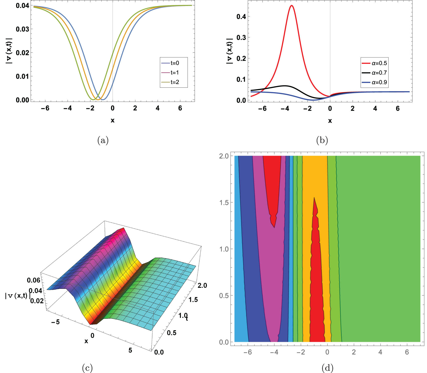
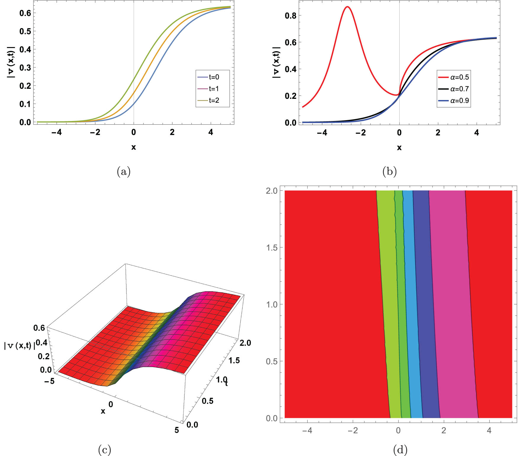
5 Physically illustrations
Here, we will provide the solutions’ physical behaviors using contour, 3D, and 2D graphs. In addition, 2D graphs are created for various
(Kink soliton solution) graph of
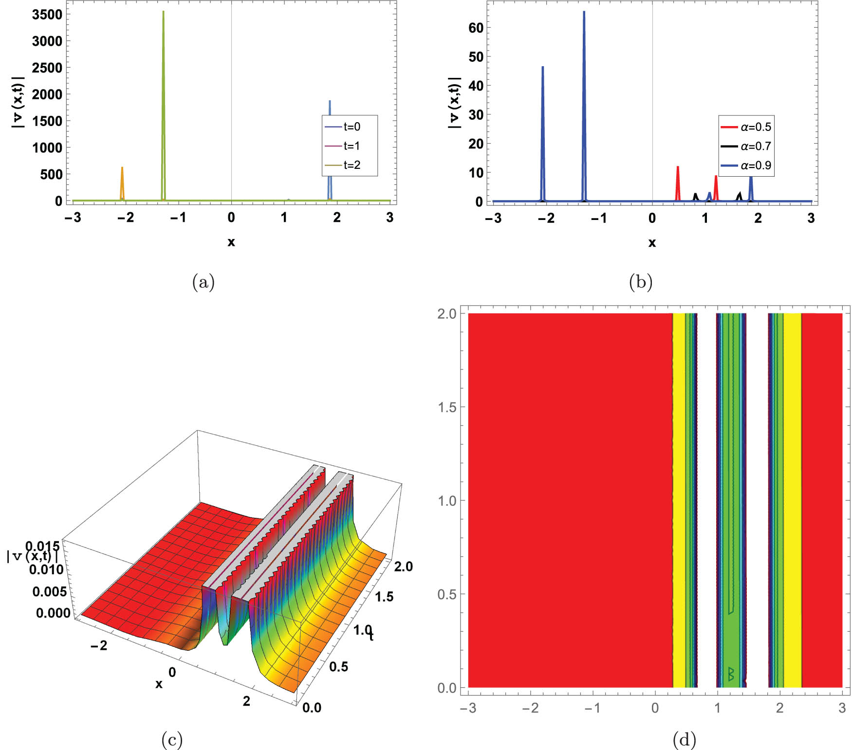
(Periodic wave soliton) graph of
(Dark soliton solution) graph for
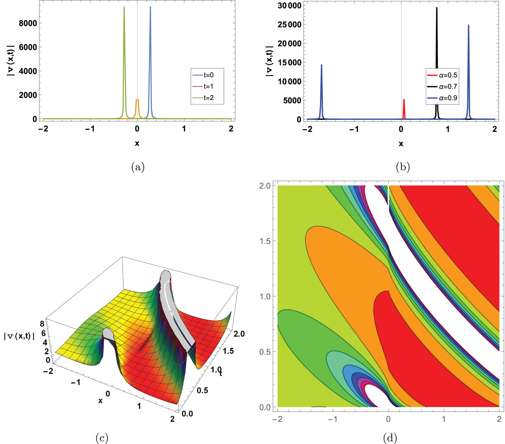
(Periodic wave solutions) graph for
6 A stability analysis
It serves to describes how the model reacts over time and how it behaves in response to outside disturbances. This analysis of various equations are explained in the literature, including [33,34].
Now, we will discuss the stability analysis of Eq. (2). For this purpose, we consider the given condition;
where
where
by using the criterion given in Eq. (58), we obtain
Hence, the given condition is fulfilled. So, Eq. (2) is a stable equation.
7 Results and discussion
Here, we give a comparative analysis of our findings alongside present solutions in the literature. Alquran et al. [20] demonstrates the acquisition of various topological and nontopological wave solutions through the application of the extended rational sinh–cosh method, the extended rational sine–cosine method, and a polynomial function method. Similarly, Butt et al. [21] successfully derived dark, bright, and periodic solitons by employing the homogeneous balance scheme.
In contrast, our research utilizes the concerned equation in conjunction along TMFD, which has enabled us to gain a diverse range of wave solitons. These include dark, periodic, and kink soliton solutions, among others, through the implementation of the unified technique and the modified simplest equation method. Kink soliton solutions have many applications, including nonlinear fibers, signal processing, electromagnetism, and complex media, etc. Periodic wave solutions are useful in plasma physics, nonlinear optics, energy harvesting, etc. Dark soliton has many applications in different fields, including ultrafast optics, nonlinear dynamics, quantum computing, etc. Furthermore, our work contributes to the field by incorporating a stability analysis of the solutions, a topic that has not been addressed in prior studies. The results we have obtained hold significant potential for future research into the model and related areas, such as nonlinear optics, telecommunications, and ocean engineering.
8 Conclusion
In this article, we successfully attained the new exact solitons of the nonlinear (1+1)-D mm-KdV equation along with a novel definition of derivative. The modified-mixed Korteweg–de Vries equation is an equation that describes a flat-topped electron distribution with more nonlinearity, which correlates to a narrower and faster wave. The solutions has been achieved through the application of unified and modified simplest equation techniques. The resulting solutions encompass a diverse array of soliton types, including dark, periodic, kink, and other soliton types. The influence of derivations on these results has also been explored, pressing the distinctness of these results in comparison to being bones. In the future, the obtained solutions can be observed experimentally like the solutions of other models [35,36].
To insure the accuracy as well as delicacy of the obtained results, Mathematica tool was used for calculation as well as verification. Also, we have shown the deduced results by two-, three-dimensional, and Contour graphs, as shown in numbers 1–4. The results are useful in different fields including, ocean engineering, fluid dynamics, etc.
Also, a stability analysis of the concerned equation has been performed to corroborate the stability and perfection of the attained results. The styles utilized are not only simple but also exceptionally effective in working nonlinear FPDEs. Likewise, these ways prove to be precious for addressing advanced-order nonlinear FPDEs. The findings presented then offer substantial perceptivity and implicit operations across different fields of science as well as engineering.
Acknowledgments
This work was supported by the Deanship of Scientific Research, Vice Presidency for Graduate Studies and Scientific Research, King Faisal University, Saudi Arabia [KFU253342].
-
Funding information: This work was supported by the Deanship of Scientific Research, Vice Presidency for Graduate Studies and Scientific Research, King Faisal University, Saudi Arabia [KFU253342].
-
Author contributions: AA: writing – funding – review and editing, conceptualization, methodology, and project administration; AAN: writing – review and editing, conceptualization, methodology; AB: writing – original draft, conceptualization, methodology, review and editing, formal analysis, and supervision. All authors have accepted responsibility for the entire content of this manuscript and approved its submission.
-
Conflict of interest: The authors state no conflict of interest.
References
[1] Wang Y-Y and Dai C-Q. Elastic interactions between multi-valued foldons and anti-foldons for the (2+1)-dimensional variable coefficient Broer-Kaup system in water waves. Nonlinear Dyn. 2013;74:429–38. 10.1007/s11071-013-0980-ySearch in Google Scholar
[2] Kong L-Q and Dai C-Q. Some discussions about variable separation of nonlinear models using Riccati equation expansion method. Nonlinear Dyn. 2015;81:1553–61. 10.1007/s11071-015-2089-ySearch in Google Scholar
[3] Khater MMA. Novel constructed dark, bright and rogue waves of three models of the well-known nonlinear Schrödinger equation. Int J Modern Phys B. 2024;38(3):2450023. 10.1142/S0217979224500231Search in Google Scholar
[4] Khater MMA. Exploring the rich solution landscape of the generalized Kawahara equation: Insights from analytical techniques. Europ Phys J Plus. 2024;139(2):184. 10.1140/epjp/s13360-024-04971-0Search in Google Scholar
[5] Khater MMA. Computational method for obtaining solitary wave solutions of the (2+1)-dimensional AKNS equation and their physical significance. Modern Phys Lett B. 2024;38(19):2350252. 10.1142/S0217984923502524Search in Google Scholar
[6] Khater M. Dynamics of nonlinear time fractional equations in shallow water waves. Int J Theoret Phys. 2024;63(4):1–12. 10.1007/s10773-024-05634-7Search in Google Scholar
[7] Walait A, Ashraf H, Chou D, Rehman HU. Stagnant rings and uniform film analysis of Phan-Thien Tanner fluid film flow on a vertically upward moving tube. Phys Fluids. 2024;36(8):083613. 10.1063/5.0218994Search in Google Scholar
[8] Khater MMA. Comment on the paper of El-Ganaini et al. [Chaos, Solitons and Fractals 140 (2020) 110218]. Chaos Solitons Fractals. 2024. 182:114729. 10.1016/j.chaos.2024.114729Search in Google Scholar
[9] Ullah MS, Abdeljabbar A, Roshid H-O, Ali MZ. Application of the unified method to solve the Biswas–Arshed model. Results Phys. 2022;42:105946. 10.1016/j.rinp.2022.105946Search in Google Scholar
[10] Chou D, Boulaaras SM, Rehman HU, Iqbal I, Akram A, Ullah N. Additional investigation of the Biswas–Arshed equation to reveal optical soliton dynamics in birefringent fiber. Opt Quant Electron. 2024;56:705. 10.1007/s11082-024-06366-ySearch in Google Scholar
[11] Wang X, Javed SA, Majeed A, Kamran M, Abbas M. Investigation of exact solutions of nonlinear evolution equations using unified method. Mathematics. 2022;10(16):2996. 10.3390/math10162996Search in Google Scholar
[12] Khater Mostafa MA. Waves in motion: unraveling nonlinear behavior through the Gilson-Pickering equation. Europ Phys J Plus. 2023;138(12):1138. 10.1140/epjp/s13360-023-04774-9Search in Google Scholar
[13] Akbari M. Exact solutions of the coupled Higgs equation and the Maccari system using the modified simplest equation method. Inform Sci Lett. 2013;2(3):155–8. 10.12785/isl/020304Search in Google Scholar
[14] Kuo C-K. New solitary solutions of the Gardner equation and Whitham-Broer-Kaup equations by the modified simplest equation method. Optik. 2017;147:128–35. 10.1016/j.ijleo.2017.08.048Search in Google Scholar
[15] Akbari M. The modified simplest equation method for finding the exact solutions of nonlinear PDEs in mathematical physics. Quantum Phys Lett. 2014;3(3):33. Search in Google Scholar
[16] Chou D, Boulaaras SM, Rehman HU, Iqbal I. Probing wave dynamics in the modified fractional nonlinear Schrödinger equation: implications for ocean engineering. Opt Quantum Electron. 2023;56:228. 10.1007/s11082-023-05954-8Search in Google Scholar
[17] Chou D, Rehman HU, Haider R, Muhammad T, Li T-L. Analyzing optical soliton propagation in perturbed nonlinear Schrödinger equation: A multi-technique study. Optik. 2024;302:171714. 10.1016/j.ijleo.2024.171714Search in Google Scholar
[18] Chou D, UrRehman H, Amer A, Amer A. New solitary wave solutions of generalized fractional Tzitzéica-type evolution equations using sardar sub-equation method. Opt Quantum Electron. 2023;55:1148. 10.1007/s11082-023-05425-0Search in Google Scholar
[19] Bibi A, Shakeel M, Khan D, Hussain S, Chou D. Study of solitary and kink waves, stability analysis, and fractional effect in magnetized plasma. Results Phys. 2023;44:106166. 10.1016/j.rinp.2022.106166Search in Google Scholar
[20] Alquran M, Ali M, Jadallah H. New topological and non-topological unidirectional-wave solutions for the modified-mixed KdV equation and bidirectional-waves solutions for the Benjamin Ono equation using recent techniques. J Ocean Eng Sci. 2022;7(2):163–9. 10.1016/j.joes.2021.07.008Search in Google Scholar
[21] Butt AR, Raza N, Ahmad H, Ozsahin DU, Tchier F, et al. Different solitary wave solutions and bilinear form for modified mixed-KDV equation. Optik. 2023;287:171031. 10.1016/j.ijleo.2023.171031Search in Google Scholar
[22] Sulaiman TA, Yel G, Bulut H. M-fractional solitons and periodic wave solutions to the Hirota-Maccari system. Modern Phys Lett B. 2019;33:1950052. 10.1142/S0217984919500520Search in Google Scholar
[23] Vanterler da C. Sousa J, Capelas de Oliveira E. A new truncated M-fractional derivative type unifying some fractional derivative types with classical properties. Int J Anal Appl. 2018;16(1):83–96. Search in Google Scholar
[24] Qawaqneh H, Zafar A, Raheel M, Zaagan AA, Zahran EHM, Cevikel A, et al. New soliton solutions of M-fractional Westervelt model in ultrasound imaging via two analytical techniques. Opt Quant Electron. 2024;56(5):737. 10.1007/s11082-024-06371-1Search in Google Scholar
[25] Mohammed WW, Cesarano C, Al-Askar FM. Solutions to the (4+1)-dimensional time-fractional Fokas equation with M-truncated derivative. Mathematics. 2022;11(1):194. 10.3390/math11010194Search in Google Scholar
[26] Wang K. New perspective to the fractal Konopelchenko–Dubrovsky equations with M-truncated fractional derivative. Int J Geometr Meth Modern Phys. 2023;20(5):2350072. 10.1142/S021988782350072XSearch in Google Scholar
[27] Fahad A, Boulaaras SM, Rehman HU, Iqbal I, Chou D. Probing nonlinear wave dynamics: Insights from the (2+1)-dimensional Konopelchenko–Dubrovsky. Results Phys. 2024;57:107370. 10.1016/j.rinp.2024.107370Search in Google Scholar
[28] Tagare SG, Chakrabarti A. Solution of a generalized Korteweg-de Vries equation. Phys Fluids. 1974;17(6):1331–2. 10.1063/1.1694886Search in Google Scholar
[29] Das GC, Tagare SG, Sarma J. Quasipotential analysis for ion-acoustic solitary waves and double layers in plasmas. Planet Space Sci. 1998;46(4):417–24. 10.1016/S0032-0633(97)00142-6Search in Google Scholar
[30] Sain S, Ghose-Choudhury A, Garai S. Solitary wave solutions for the KdV-type equations in plasma: a new approach with the Kudryashov function. Europ Phys J Plus. 2021;136(2):226. 10.1140/epjp/s13360-021-01217-1Search in Google Scholar
[31] Fahad A, Boulaaras SM, Rehman HU, Iqbal I, Saleem MS, Chou D. Analysing soliton dynamics and a comparative study of fractional derivatives in the nonlinear fractional Kudryashovas equation. Results Phys. 2023;55:107114. 10.1016/j.rinp.2023.107114Search in Google Scholar
[32] Shakeel M, Bibi A, Chou D, Zafar A. Study of optical solitons with Kudryashovas quintuple power law of nonlinearity using two modified techniques. Optik. 2023;273:170364. 10.1016/j.ijleo.2022.170364Search in Google Scholar
[33] Tariq KU, Wazwaz A-M, Javed R. Construction of different wave structures, stability analysis and modulation instability of the coupled nonlinear Drinfel’d-Sokolov-Wilson model. Chaos Solitons Fractals. 2023;166:112903. 10.1016/j.chaos.2022.112903Search in Google Scholar
[34] Zulfiqar H, Aashiq A, Tariq KU, Ahmad H, Almohsen B, Aslam M, et al. On the solitonic wave structures and stability analysis of the stochastic nonlinear Schrödinger equation with the impact of multiplicative noise. Optik. 2023;289:171250. 10.1016/j.ijleo.2023.171250Search in Google Scholar
[35] Si Z-Z, Wang Y-Y, Dai C-Q. Switching, explosion, and chaos of multi-wavelength soliton states in ultrafast fiber lasers. Sci China Phys Mech Astron. 2024;67(7):1–9. 10.1007/s11433-023-2365-7Search in Google Scholar
[36] Ju Z-T, Si Z-Z, Yan X, Dai C-Q. Solitons and their biperiodic pulsation in ultrafast fiber lasers based on CB/GO. Chin Phys Lett. 2024;41(8):084203. 10.1088/0256-307X/41/8/084203Search in Google Scholar
© 2025 the author(s), published by De Gruyter
This work is licensed under the Creative Commons Attribution 4.0 International License.
Articles in the same Issue
- Research Articles
- Single-step fabrication of Ag2S/poly-2-mercaptoaniline nanoribbon photocathodes for green hydrogen generation from artificial and natural red-sea water
- Abundant new interaction solutions and nonlinear dynamics for the (3+1)-dimensional Hirota–Satsuma–Ito-like equation
- A novel gold and SiO2 material based planar 5-element high HPBW end-fire antenna array for 300 GHz applications
- Explicit exact solutions and bifurcation analysis for the mZK equation with truncated M-fractional derivatives utilizing two reliable methods
- Optical and laser damage resistance: Role of periodic cylindrical surfaces
- Numerical study of flow and heat transfer in the air-side metal foam partially filled channels of panel-type radiator under forced convection
- Water-based hybrid nanofluid flow containing CNT nanoparticles over an extending surface with velocity slips, thermal convective, and zero-mass flux conditions
- Dynamical wave structures for some diffusion--reaction equations with quadratic and quartic nonlinearities
- Solving an isotropic grey matter tumour model via a heat transfer equation
- Study on the penetration protection of a fiber-reinforced composite structure with CNTs/GFP clip STF/3DKevlar
- Influence of Hall current and acoustic pressure on nanostructured DPL thermoelastic plates under ramp heating in a double-temperature model
- Applications of the Belousov–Zhabotinsky reaction–diffusion system: Analytical and numerical approaches
- AC electroosmotic flow of Maxwell fluid in a pH-regulated parallel-plate silica nanochannel
- Interpreting optical effects with relativistic transformations adopting one-way synchronization to conserve simultaneity and space–time continuity
- Modeling and analysis of quantum communication channel in airborne platforms with boundary layer effects
- Theoretical and numerical investigation of a memristor system with a piecewise memductance under fractal–fractional derivatives
- Tuning the structure and electro-optical properties of α-Cr2O3 films by heat treatment/La doping for optoelectronic applications
- High-speed multi-spectral explosion temperature measurement using golden-section accelerated Pearson correlation algorithm
- Dynamic behavior and modulation instability of the generalized coupled fractional nonlinear Helmholtz equation with cubic–quintic term
- Study on the duration of laser-induced air plasma flash near thin film surface
- Exploring the dynamics of fractional-order nonlinear dispersive wave system through homotopy technique
- The mechanism of carbon monoxide fluorescence inside a femtosecond laser-induced plasma
- Numerical solution of a nonconstant coefficient advection diffusion equation in an irregular domain and analyses of numerical dispersion and dissipation
- Numerical examination of the chemically reactive MHD flow of hybrid nanofluids over a two-dimensional stretching surface with the Cattaneo–Christov model and slip conditions
- Impacts of sinusoidal heat flux and embraced heated rectangular cavity on natural convection within a square enclosure partially filled with porous medium and Casson-hybrid nanofluid
- Stability analysis of unsteady ternary nanofluid flow past a stretching/shrinking wedge
- Solitonic wave solutions of a Hamiltonian nonlinear atom chain model through the Hirota bilinear transformation method
- Bilinear form and soltion solutions for (3+1)-dimensional negative-order KdV-CBS equation
- Solitary chirp pulses and soliton control for variable coefficients cubic–quintic nonlinear Schrödinger equation in nonuniform management system
- Influence of decaying heat source and temperature-dependent thermal conductivity on photo-hydro-elasto semiconductor media
- Dissipative disorder optimization in the radiative thin film flow of partially ionized non-Newtonian hybrid nanofluid with second-order slip condition
- Bifurcation, chaotic behavior, and traveling wave solutions for the fractional (4+1)-dimensional Davey–Stewartson–Kadomtsev–Petviashvili model
- New investigation on soliton solutions of two nonlinear PDEs in mathematical physics with a dynamical property: Bifurcation analysis
- Mathematical analysis of nanoparticle type and volume fraction on heat transfer efficiency of nanofluids
- Creation of single-wing Lorenz-like attractors via a ten-ninths-degree term
- Optical soliton solutions, bifurcation analysis, chaotic behaviors of nonlinear Schrödinger equation and modulation instability in optical fiber
- Chaotic dynamics and some solutions for the (n + 1)-dimensional modified Zakharov–Kuznetsov equation in plasma physics
- Fractal formation and chaotic soliton phenomena in nonlinear conformable Heisenberg ferromagnetic spin chain equation
- Single-step fabrication of Mn(iv) oxide-Mn(ii) sulfide/poly-2-mercaptoaniline porous network nanocomposite for pseudo-supercapacitors and charge storage
- Novel constructed dynamical analytical solutions and conserved quantities of the new (2+1)-dimensional KdV model describing acoustic wave propagation
- Tavis–Cummings model in the presence of a deformed field and time-dependent coupling
- Spinning dynamics of stress-dependent viscosity of generalized Cross-nonlinear materials affected by gravitationally swirling disk
- Design and prediction of high optical density photovoltaic polymers using machine learning-DFT studies
- Robust control and preservation of quantum steering, nonlocality, and coherence in open atomic systems
- Coating thickness and process efficiency of reverse roll coating using a magnetized hybrid nanomaterial flow
- Dynamic analysis, circuit realization, and its synchronization of a new chaotic hyperjerk system
- Decoherence of steerability and coherence dynamics induced by nonlinear qubit–cavity interactions
- Finite element analysis of turbulent thermal enhancement in grooved channels with flat- and plus-shaped fins
- Modulational instability and associated ion-acoustic modulated envelope solitons in a quantum plasma having ion beams
- Statistical inference of constant-stress partially accelerated life tests under type II generalized hybrid censored data from Burr III distribution
- On solutions of the Dirac equation for 1D hydrogenic atoms or ions
- Entropy optimization for chemically reactive magnetized unsteady thin film hybrid nanofluid flow on inclined surface subject to nonlinear mixed convection and variable temperature
- Stability analysis, circuit simulation, and color image encryption of a novel four-dimensional hyperchaotic model with hidden and self-excited attractors
- A high-accuracy exponential time integration scheme for the Darcy–Forchheimer Williamson fluid flow with temperature-dependent conductivity
- Novel analysis of fractional regularized long-wave equation in plasma dynamics
- Development of a photoelectrode based on a bismuth(iii) oxyiodide/intercalated iodide-poly(1H-pyrrole) rough spherical nanocomposite for green hydrogen generation
- Investigation of solar radiation effects on the energy performance of the (Al2O3–CuO–Cu)/H2O ternary nanofluidic system through a convectively heated cylinder
- Quantum resources for a system of two atoms interacting with a deformed field in the presence of intensity-dependent coupling
- Studying bifurcations and chaotic dynamics in the generalized hyperelastic-rod wave equation through Hamiltonian mechanics
- A new numerical technique for the solution of time-fractional nonlinear Klein–Gordon equation involving Atangana–Baleanu derivative using cubic B-spline functions
- Interaction solutions of high-order breathers and lumps for a (3+1)-dimensional conformable fractional potential-YTSF-like model
- Hydraulic fracturing radioactive source tracing technology based on hydraulic fracturing tracing mechanics model
- Numerical solution and stability analysis of non-Newtonian hybrid nanofluid flow subject to exponential heat source/sink over a Riga sheet
- Numerical investigation of mixed convection and viscous dissipation in couple stress nanofluid flow: A merged Adomian decomposition method and Mohand transform
- Effectual quintic B-spline functions for solving the time fractional coupled Boussinesq–Burgers equation arising in shallow water waves
- Analysis of MHD hybrid nanofluid flow over cone and wedge with exponential and thermal heat source and activation energy
- Solitons and travelling waves structure for M-fractional Kairat-II equation using three explicit methods
- Impact of nanoparticle shapes on the heat transfer properties of Cu and CuO nanofluids flowing over a stretching surface with slip effects: A computational study
- Computational simulation of heat transfer and nanofluid flow for two-sided lid-driven square cavity under the influence of magnetic field
- Irreversibility analysis of a bioconvective two-phase nanofluid in a Maxwell (non-Newtonian) flow induced by a rotating disk with thermal radiation
- Hydrodynamic and sensitivity analysis of a polymeric calendering process for non-Newtonian fluids with temperature-dependent viscosity
- Exploring the peakon solitons molecules and solitary wave structure to the nonlinear damped Kortewege–de Vries equation through efficient technique
- Modeling and heat transfer analysis of magnetized hybrid micropolar blood-based nanofluid flow in Darcy–Forchheimer porous stenosis narrow arteries
- Activation energy and cross-diffusion effects on 3D rotating nanofluid flow in a Darcy–Forchheimer porous medium with radiation and convective heating
- Insights into chemical reactions occurring in generalized nanomaterials due to spinning surface with melting constraints
- Influence of a magnetic field on double-porosity photo-thermoelastic materials under Lord–Shulman theory
- Soliton-like solutions for a nonlinear doubly dispersive equation in an elastic Murnaghan's rod via Hirota's bilinear method
- Analytical and numerical investigation of exact wave patterns and chaotic dynamics in the extended improved Boussinesq equation
- Nonclassical correlation dynamics of Heisenberg XYZ states with (x, y)-spin--orbit interaction, x-magnetic field, and intrinsic decoherence effects
- Exact traveling wave and soliton solutions for chemotaxis model and (3+1)-dimensional Boiti–Leon–Manna–Pempinelli equation
- Unveiling the transformative role of samarium in ZnO: Exploring structural and optical modifications for advanced functional applications
- On the derivation of solitary wave solutions for the time-fractional Rosenau equation through two analytical techniques
- Analyzing the role of length and radius of MWCNTs in a nanofluid flow influenced by variable thermal conductivity and viscosity considering Marangoni convection
- Advanced mathematical analysis of heat and mass transfer in oscillatory micropolar bio-nanofluid flows via peristaltic waves and electroosmotic effects
- Exact bound state solutions of the radial Schrödinger equation for the Coulomb potential by conformable Nikiforov–Uvarov approach
- Some anisotropic and perfect fluid plane symmetric solutions of Einstein's field equations using killing symmetries
- Nonlinear dynamics of the dissipative ion-acoustic solitary waves in anisotropic rotating magnetoplasmas
- Curves in multiplicative equiaffine plane
- Exact solution of the three-dimensional (3D) Z2 lattice gauge theory
- Propagation properties of Airyprime pulses in relaxing nonlinear media
- Symbolic computation: Analytical solutions and dynamics of a shallow water wave equation in coastal engineering
- Wave propagation in nonlocal piezo-photo-hygrothermoelastic semiconductors subjected to heat and moisture flux
- Comparative reaction dynamics in rotating nanofluid systems: Quartic and cubic kinetics under MHD influence
- Laplace transform technique and probabilistic analysis-based hypothesis testing in medical and engineering applications
- Physical properties of ternary chloro-perovskites KTCl3 (T = Ge, Al) for optoelectronic applications
- Gravitational length stretching: Curvature-induced modulation of quantum probability densities
- The search for the cosmological cold dark matter axion – A new refined narrow mass window and detection scheme
- A comparative study of quantum resources in bipartite Lipkin–Meshkov–Glick model under DM interaction and Zeeman splitting
- PbO-doped K2O–BaO–Al2O3–B2O3–TeO2-glasses: Mechanical and shielding efficacy
- Nanospherical arsenic(iii) oxoiodide/iodide-intercalated poly(N-methylpyrrole) composite synthesis for broad-spectrum optical detection
- Sine power Burr X distribution with estimation and applications in physics and other fields
- Numerical modeling of enhanced reactive oxygen plasma in pulsed laser deposition of metal oxide thin films
- Dynamical analyses and dispersive soliton solutions to the nonlinear fractional model in stratified fluids
- Computation of exact analytical soliton solutions and their dynamics in advanced optical system
- An innovative approximation concerning the diffusion and electrical conductivity tensor at critical altitudes within the F-region of ionospheric plasma at low latitudes
- An analytical investigation to the (3+1)-dimensional Yu–Toda–Sassa–Fukuyama equation with dynamical analysis: Bifurcation
- Swirling-annular-flow-induced instability of a micro shell considering Knudsen number and viscosity effects
- Numerical analysis of non-similar convection flows of a two-phase nanofluid past a semi-infinite vertical plate with thermal radiation
- MgO NPs reinforced PCL/PVC nanocomposite films with enhanced UV shielding and thermal stability for packaging applications
- Optimal conditions for indoor air purification using non-thermal Corona discharge electrostatic precipitator
- Investigation of thermal conductivity and Raman spectra for HfAlB, TaAlB, and WAlB based on first-principles calculations
- Tunable double plasmon-induced transparency based on monolayer patterned graphene metamaterial
- DSC: depth data quality optimization framework for RGBD camouflaged object detection
- A new family of Poisson-exponential distributions with applications to cancer data and glass fiber reliability
- Numerical investigation of couple stress under slip conditions via modified Adomian decomposition method
- Monitoring plateau lake area changes in Yunnan province, southwestern China using medium-resolution remote sensing imagery: applicability of water indices and environmental dependencies
- Heterodyne interferometric fiber-optic gyroscope
- Exact solutions of Einstein’s field equations via homothetic symmetries of non-static plane symmetric spacetime
- A widespread study of discrete entropic model and its distribution along with fluctuations of energy
- Empirical model integration for accurate charge carrier mobility simulation in silicon MOSFETs
- The influence of scattering correction effect based on optical path distribution on CO2 retrieval
- Anisotropic dissociation and spectral response of 1-Bromo-4-chlorobenzene under static directional electric fields
- Role of tungsten oxide (WO3) on thermal and optical properties of smart polymer composites
- Analysis of iterative deblurring: no explicit noise
- The influence of anisotropy of InP on its elasticity and phonon properties
- Review Article
- Examination of the gamma radiation shielding properties of different clay and sand materials in the Adrar region
- Erratum
- Erratum to “On Soliton structures in optical fiber communications with Kundu–Mukherjee–Naskar model (Open Physics 2021;19:679–682)”
- Special Issue on Fundamental Physics from Atoms to Cosmos - Part II
- Possible explanation for the neutron lifetime puzzle
- Special Issue on Nanomaterial utilization and structural optimization - Part III
- Numerical investigation on fluid-thermal-electric performance of a thermoelectric-integrated helically coiled tube heat exchanger for coal mine air cooling
- Special Issue on Nonlinear Dynamics and Chaos in Physical Systems
- Analysis of the fractional relativistic isothermal gas sphere with application to neutron stars
- Abundant wave symmetries in the (3+1)-dimensional Chafee–Infante equation through the Hirota bilinear transformation technique
- Successive midpoint method for fractional differential equations with nonlocal kernels: Error analysis, stability, and applications
- Novel exact solitons to the fractional modified mixed-Korteweg--de Vries model with a stability analysis