New investigation on soliton solutions of two nonlinear PDEs in mathematical physics with a dynamical property: Bifurcation analysis
-
 ,
,

Abstract
To comprehend nonlinear dynamics, one must have access to soliton solutions, which faithfully portray the actions of numerous physical systems and nonlinear equations. Notable nonlinear equations in relativistic physics, quantum field theory, nonlinear optics, dispersive wave phenomena, contemporary industrial applications, and plasma physics include the Klein–Gordon and Sharma–Tasso–Olver equations, which shed light on wave behavior and interactions. This study introduces a powerful approach to uncovering some novel soliton solutions for these equations, namely, the new generalized
1 Introduction
The natural world exhibits a range of complex physical phenomena, from fluid dynamics and light propagation to plasma behavior and ecosystem interactions. These diverse phenomena are often effectively described by nonlinear key equations, which capture the intricate interdependencies and interactions inherent in such systems. A crucial category of these equations is the nonlinear evolution equations (NLEEs), a specific subset of partial differential equations (PDEs). NLEEs play a significant role in mathematical physics, applied mathematics, and engineering. They are particularly valuable for modeling dynamic processes in various fields: quantum mechanics, where they describe the evolution of quantum states; nonlinear optics, where they capture the propagation of light pulses through optical fibers; plasma physics, where they help understand the behavior of charged particles in electromagnetic fields; biophysics, where they model biological patterns and structures; and ecology, where they describe population dynamics and species spread [1,2,3,4,5].
Given their broad applicability, NLEEs are central to research in nonlinear science. They enable the modeling of phenomena where linear approximations are inadequate, particularly when interactions, feedback mechanisms, or other nonlinear effects are involved. Finding exact solutions to these equations provides critical insights into the nature and properties of physical systems, revealing stable configurations like solitons, shock waves, and traveling waves. Such solutions are essential for validating numerical simulations and providing benchmarks for approximations. Among NLEEs, the Klein–Gordon (KG) equation and the Sharma–Tasso–Olver (STO) equation are notable for their roles in nonlinear dynamics, offering significant insights into wave behavior and interactions. Investigating these exact solutions is not just a theoretical pursuit but a key aspect of advancing our understanding of complex systems and developing new technologies [6,7,8,9,10].
The KG equation is a fundamental relativistic wave equation in quantum field theory that characterizes scalar particles, such as the Higgs boson and specific mesons, which possess no intrinsic spin. Designed to reconcile quantum mechanics with special relativity, it guarantees the uniform behavior of particles in all inertial frames. Initially designed to represent the wave function of a single particle, it was discovered to encompass both positive and negative energy solutions, which presented conceptual difficulties. This issue was addressed by reinterpreting the equation within quantum field theory to depict fields that generate and annihilate particles, with negative energy solutions representing antiparticles. This reinterpretation corresponds with discoveries in particle physics, where each particle possesses a corresponding antiparticle. The KG equation is crucial in both particle physics and cosmology, as it delineates scalar fields pertinent to cosmic inflation and dark energy, so linking the quantum realm with the universe’s large-scale structure and evolution. Due to its importance, several academics have addressed the KG equation to derive soliton solutions through diverse methodologies [11,12,13,14,15]. Some of the methods employed to find these solutions include the Sobolev gradients technique [11], the Jacobi elliptic function method [12], the F-expansion method [13], the Exp-function technique [14], and the Homotopy analysis technique [15], among others. Each of these techniques offers a unique pathway to derive exact or approximate solutions, enhancing our understanding of soliton behavior in nonlinear dynamics.
The STO equation is a nonlinear partial differential equation that plays a significant role in understanding wave phenomena across various scientific fields, including fluid dynamics, nonlinear optics, and plasma physics. As an integrable system, it can be solved exactly using advanced mathematical techniques such as the inverse scattering transform (IST) and Hirota’s direct method. This exact solvability allows researchers to explore soliton solutions, which are stable, localized waves that retain their shape and speed even after interacting with other waves. The STO equation is particularly valuable for modeling systems where both nonlinearity and dispersion are important, such as shallow water waves, nonlinear lattice dynamics, and optical pulse propagation in fibers. Its ability to describe complex wave behavior makes it a critical tool in both theoretical studies and practical applications, offering insights into how nonlinear waves evolve, interact, and propagate in various media. The STO equation helps in predicting and controlling wave dynamics, enhancing our understanding of wave-based phenomena in both natural and engineered systems. The STO equation has recently attracted significant interest from the scientific community for its crucial role in modeling traveling-wave phenomena [16,17,18,19,20,21,22,23,24]. This equation is widely applied in fields such as nonlinear optics [16], plasma physics [17], dispersive wave dynamics [18], conservation laws [19], Lie symmetry analysis [20], and quantum field theory [21]. In particular, Wang [22] investigated the dynamic characteristics of the STO model and assessed the stability of its traveling wave solutions using the spectral energy estimate method. Additionally, Wang and Xu [23] employed the Lie group analysis method to find exact and explicit solutions to the STO equation, enhancing our understanding of its complex behavior. The soliton solutions of the STO equation are particularly noteworthy, as they demonstrate unique behaviors like the capacity to split into several solitons or merge into one under certain conditions [24].
Given the importance and significance of NLEEs in various fields, researchers have developed and expanded numerous techniques for deriving their exact solutions over recent years. For example: the double
In a recent development, Naher et al. [39] introduced the new generalized
Comparison of present method with other established methods
| Method | Strengths | Limitations | Advantages of present method |
|---|---|---|---|
| Hirota’s method | Multi-soliton solutions | Requires bilinearization, works best for integrable equations | No need for bilinear form, works for broader equations |
| IST | Exact soliton solutions for integrable systems | Complex spectral analysis, applies only to integrable equations | No spectral transforms needed, applicable to non-integrable PDEs |
| Tanh-Coth method | Hyperbolic solutions | Limited to certain forms of PDEs | Gives more diverse function solutions |
| Sine-Cosine method | Trigonometric solutions | Better works mainly for periodic waves | More general wave solutions |
| Exp-Function method | Very simple for some PDEs | Does not always capture all solutions | More systematic algebraic structure |
Consequently, the objective of this investigation is to investigate novel exact solutions for both the KG equation and the STO equation by employing this methodology. The study is structured as follows: initially, we present an introduction to the methods, which is followed by the application of the method to the aforementioned equations to identify soliton solutions. Subsequently, we discuss the bifurcation analysis of the dynamical system corresponding to those equations. The following section delves into the graphical behavior of the solitons that were obtained and compares our results to those of previous studies. The study concludes with a reference section that lists the sources that contributed to this research and a summary of our findings.
2 Interpretation of the method
The new generalized
Suppose the general form of the NLEEs is
where
Step 1: We consider the combination of real variables
(2)where
(3)where
Step 2: Depending on the situation, Eq. (3) can be integrated term by term, potentially multiple times, with the integration constant possibly being zero. This approach is suitable as we are specifically seeking solitary wave solutions.
Step 3: The traveling wave solution of Eq. (3) can be expressed as a polynomial of the following form:
(4)where either
Here
(5)where
(6)where prime indicates the derivative with respect to
Step 4: To determine the positive integer
Step 5: Inserting Eqs. (4) and (6) including Eq. (5) into Eq. (3) and utilizing the value of
Step 7: Using the general solution of Eq. (6), we obtain
Family 1: Hyperbolic function solution, where
Family 2: Trigonometric solution, when
Family 3: When
Family 4: Hyperbolic function solution, when
Family 5: Trigonometric solution, when
These are the general solutions of
3 Applications
In this section, we explain two applications of the mentioned method to extract abundant soliton solutions in Sections 3.1 and 3.2.
3.1 KG equation
Let us consider the KG equation of the form [11,12]
Eq. (12) can be converted to the following ODE via the transformation
Now the homogeneous balance between the highest order nonlinear term
where
Set 1:
Set 2:
Set 3:
Set 4:
Set 1: The constant values arranged in Eq. (15) should be inserted in Eq. (14), as well as Eq. (7) and simplifying, for both
where
In a similar fashion, substituting the values of the constants arranged in Eq. (15) in (14), as well as Eqs. (8)–(11) and simplifying, for
Set 2: Substituting the values of the constants held in Eqs (16) in (14), along with Eq. (7) and simplifying, we obtain the following traveling wave solutions for
where
Similarly, by substituting the values of the constants contained in Eq. (16) in (14), together with Eqs. (8)–(11) and simplifying, we obtain respectively the following traveling wave solutions for
Set 3: Inserting the values of the constants from Eq. (17) in (14), as well as Eqs. (7)–(11) and simplifying, we obtain the following traveling wave solutions for
where
Set 4: In a similar fashion, replacing the values of the parameters from Eq. (18) in Eq. (14), including Eqs. (7)–(11) and simplifying, we obtain the following traveling wave solutions for
where
3.2 STO equation
The STO equation comprises evenly the double nonlinear terms
Now, we reduce Eq. (19) into an ODE by choosing the transformation
Thus, integrating Eq. (20) with respect to
where
where
where
where
where
Similarly, for set 1:
Substituting the values of the constants provided in Eq. (23) in (22), including Eqs. (8)–(11) and simplifying, we obtain the following traveling wave solutions for
Similarly, for set 2:
Similarly, for set 3:
Similarly, for set 4:
Similarly, for set 5:
where,
4 Bifurcation analysis
Bifurcation analysis is an important tool for understanding the qualitative changes in nonlinear dynamical systems that support physical events. It investigates how changes in system characteristics cause shifts in equilibrium, stability, or the creation of complex behaviors like oscillations or chaos. These changes, known as bifurcations, are essential for modeling and studying critical physical processes such as phase transitions, fluid instabilities, and wave propagation. Physicists can predict and define system behavior under different conditions by finding critical points and categorizing bifurcations. Additionally, bifurcation analysis simplifies the study of intricate physical models by exposing common patterns among seemingly unrelated systems. It is essential for gaining understanding of theoretical models and directing experimental investigations of the related phenomenon because it offers a rigorous framework for investigating the relationships between stability, symmetry, and nonlinear interactions [50,51,52,53]. A brief bifurcation analysis of the KG and STO equations is given in this section. It is regarded as a planner dynamical system in this sense and can have the following forms:
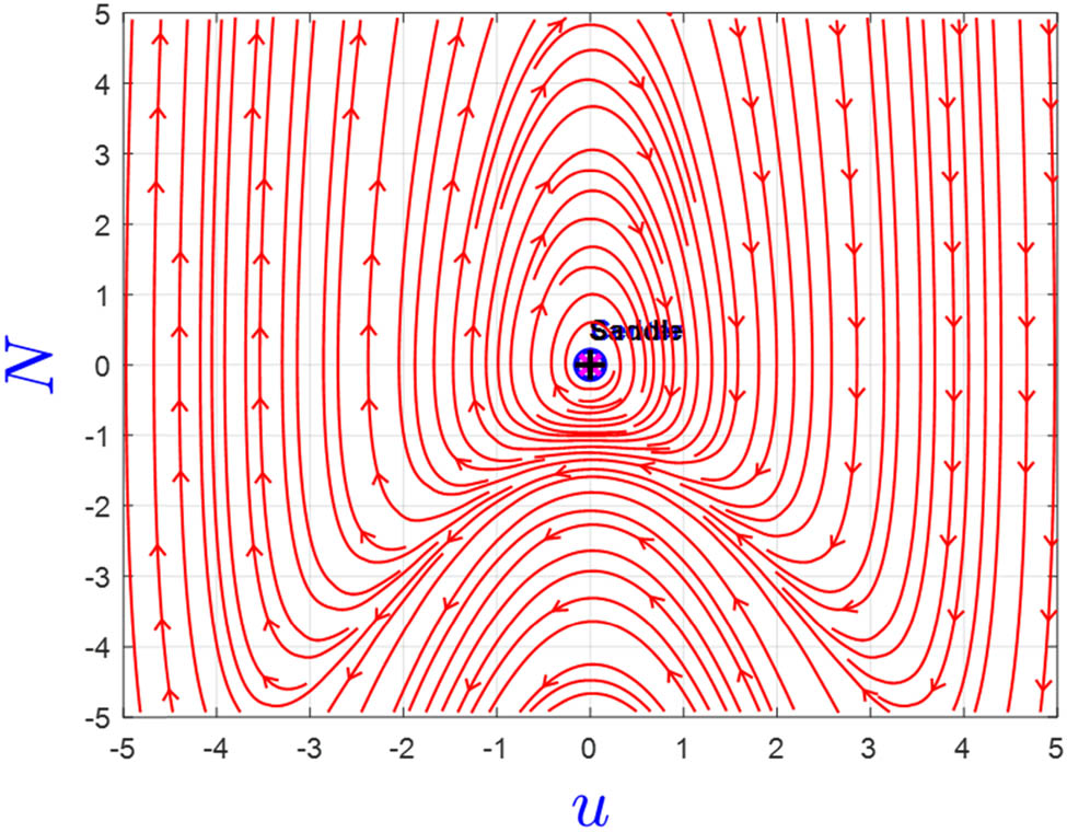
4.1 KG equation
Eq. (13) is used to define the planner dynamical system in this instance as follows:
where
To analyze the phase portrait of this system, it is crucial to first determine the equilibrium points by setting the derivatives
Case I: When

Phase behavior of Eq. (32) when
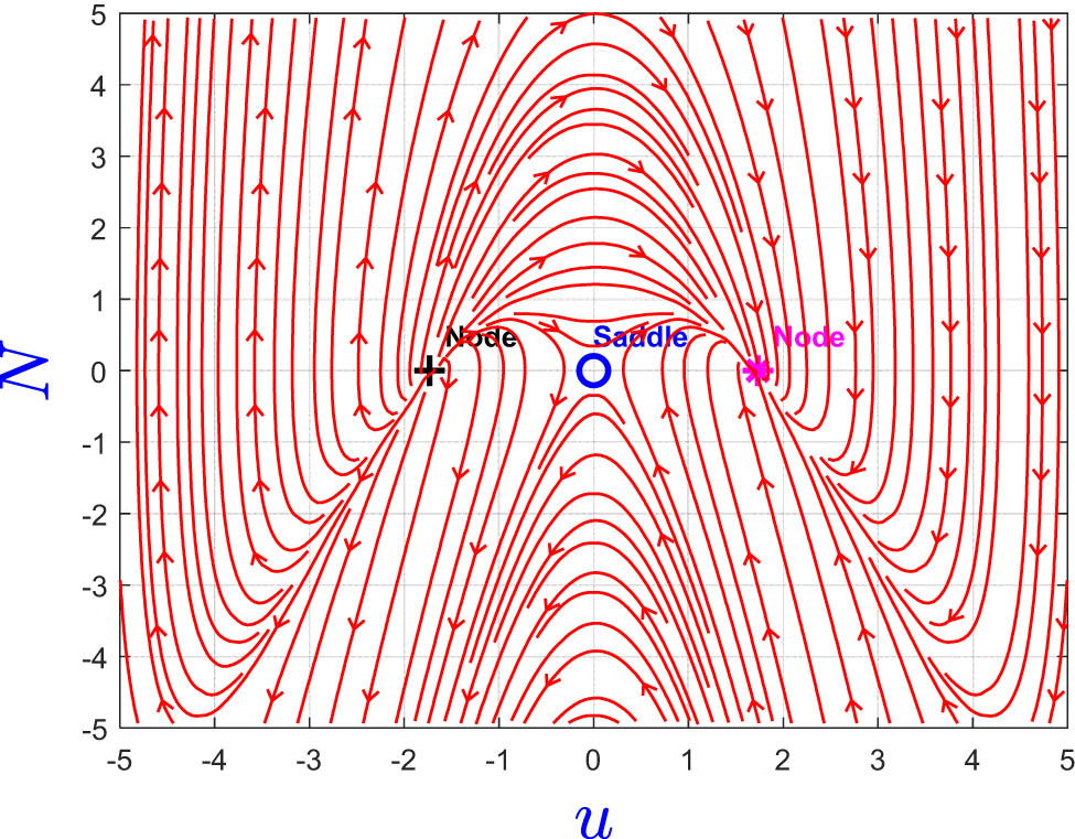
Case II: When

Phase behavior of Eq. (32) when
Case III: When
4.2 STO equation
Eq. (13) serves as the basis for defining the planar dynamical system in this case considering that the integrating constant is zero that gives
where
Similarly, the equilibrium points for this system are determined as
Case I: When
Phase behavior of Eq. (33) when
Case II: When
Phase behavior of Eq. (33) when
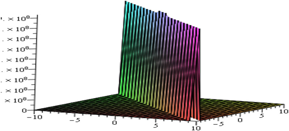
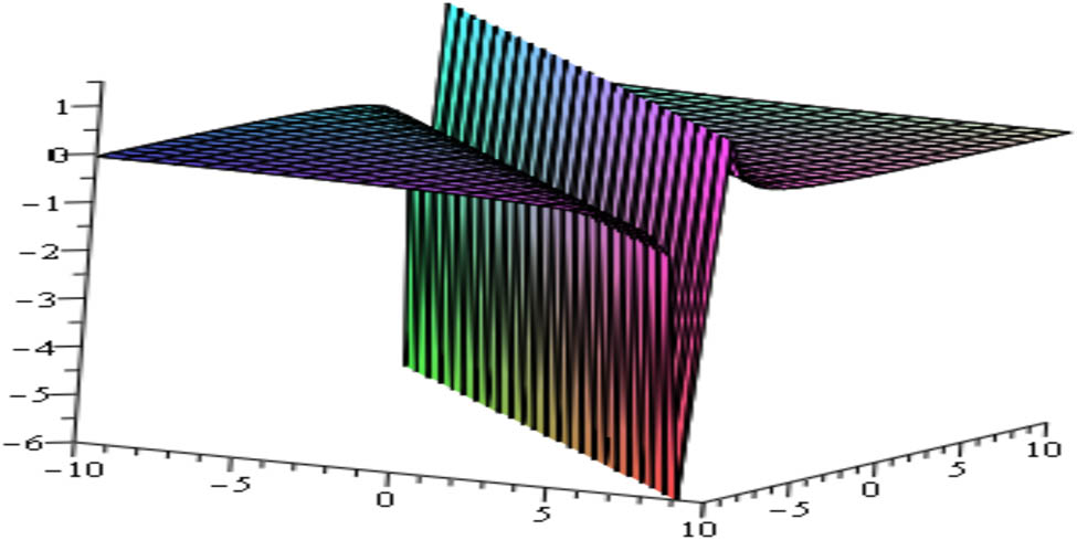
5 Discussion and graphical representations of the solutions
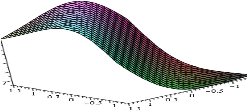
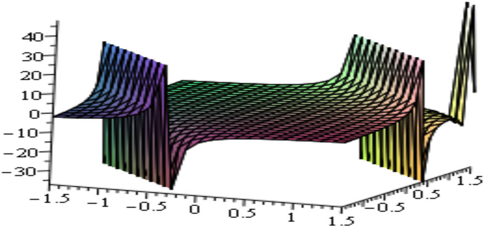
The solutions obtained through this method are straightforward and easier to interpret, effectively capturing the mechanisms underlying complex nonlinear physical phenomena. Graphical representations play a crucial role in simplifying and clarifying these solutions, providing a visual means to understand the dynamics involved in such phenomena. The graphical illustrations of some of the derived traveling wave solutions are presented in Figures 5–10, generated using computational tools like Maple. These visualizations help to clearly demonstrate the behavior of the solutions over time and space, offering valuable insights into their properties, such as amplitude, frequency, and wave speed. By employing graphical tools, the intricate nature of the solutions becomes more accessible, allowing for a deeper understanding of the nonlinear dynamics they represent.
Shape of sharp soliton of
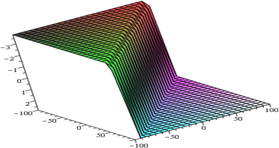
Shape of kink soliton of

Shape of the singular periodic soliton of
Shape of the singular kink soliton of
Shape of flat kink soliton of
Shape of periodic kink soliton of
The graphical analysis reveals that when the velocity of the traveling wave is set to 1, the resulting graphs of the obtained solutions clearly exhibit characteristics of an exact kink soliton, a singular kink soliton, and singular periodic solutions. However, as the velocity of the traveling wave deviates from this value, the shapes of the graphs begin to deform, indicating changes in the structure and behavior of the solutions.
In soliton dynamics, these soliton solutions provide important insights and have practical applications across multiple disciplines. Sharp solitons play a critical role in optical fibers by preserving the shape of light pulses over long distances, which is essential for high-speed data transmission [34,54]. They also aid in understanding solitary waves in shallow water systems. Kink solitons, characterized by their smooth transitions, are important in field theory and particle physics for representing domain walls, and they also describe gradual changes in light intensity in nonlinear optics [4,55]. Singular periodic solitons, which feature periodic patterns with singularities, are valuable for studying wave behavior in media with periodic structures and defects, such as optical lattices and plasma environments [2,56]. Singular kink solitons, which combine kink-like transitions with singular features, are useful for analyzing shock waves and boundary interfaces. Flat kink solitons, exhibiting constant amplitude with sharp transitions, are applied in examining phase changes in materials and stable light pulses in nonlinear optics [8,9]. Finally, periodic kink solitons, with their periodic structures and kink-like transitions, are employed to investigate wave propagation in periodic media and lattice systems, enhancing the understanding of phenomena in condensed matter physics [28,30]. Each soliton type contributes to a comprehensive understanding of complex systems and supports the advancement of both theoretical research and practical applications.
6 Conclusion
In conclusion, this study highlights the effectiveness of the new generalized
Acknowledgments
The researchers would like to thank the Deanship of Graduate Studies and Scientific Research at the Qassim University for financial support (QU-APC-2025).
-
Funding information: The researchers would like to thank the Deanship of Graduate Studies and Scientific Research at the Qassim University for financial support (QU-APC-2025).
-
Author contributions: M.D.H, S.M.B., A.M.S., H.G., and M.N.H. wrote the main manuscript text, and M.M.M. prepared all the figures and supervised this research. All authors reviewed the manuscript and have accepted responsibility for the entire content of this manuscript and approved its submission.
-
Conflict of interest: The authors state no conflicts of interest.
-
Data availability statement: All data generated or analyzed during this study are included in this published article.
References
[1] Miah MM, Iqbal MA, Osman MS. A study on stochastic longitudinal wave equation in a magneto-electro-elastic annular bar to find the analytical solutions. Commun Theor Phys. 2023;75:085008.10.1088/1572-9494/ace155Search in Google Scholar
[2] Hossain MN, Miah MM, Alosaimi M, Alsharif F, Kanan M. Exploring novel soliton solutions to the time-fractional coupled Drinfel’d-Sokolov-Wilson equation in industrial engineering using two efficient techniques. Fractal Front. 2024;8:352. 10.3390/fractalfract8060352.Search in Google Scholar
[3] Rasid MM, Miah MM, Ganie AH, Alshehri HM, Osman MS, Ma WX. Further advanced investigation of the complex Hirota-dynamical model to extract soliton solutions. Mod Phys Lett B. 2024;38(10):2450074.10.1142/S021798492450074XSearch in Google Scholar
[4] Hossain MN, Miah MM, Hamid A, Osman GMS. Discovering new abundant optical solutions for the resonant nonlinear Schrödinger equation using an analytical technique. Opt Quantum Electron. 2024;56:847.10.1007/s11082-024-06351-5Search in Google Scholar
[5] Mia R, Miah MM, Osman MS. A new implementation of a novel analytical method for finding the analytical solutions of the (2 + 1)-dimensional KP-BBM equation. Heliyon. 2023;9:e15690.10.1016/j.heliyon.2023.e15690Search in Google Scholar PubMed PubMed Central
[6] Mohamed MZ, Hamza AE, SedeegA KH. Conformable double Sumudu transformations an efficient approximation solutions to the fractional coupled Burger’s equation. Ain Shams Eng J. 2023;14:101879.10.1016/j.asej.2022.101879Search in Google Scholar
[7] Shakeel M, Attaullah, Shah NA, Chung JD. Application of modified exp-function method for strain wave equation for finding analytical solutions. Ain Shams Eng J. 2023;14:101883.10.1016/j.asej.2022.101883Search in Google Scholar
[8] Eidinejad Z, Saadati R, Li C, Inc M, Vahid J. The multiple exp-function method to obtain soliton solutions of the conformable Date-Jimbo-Kashiwara-Miwa equations. Int J Mod Phys B. 2023;38(3):2450043.10.1142/S0217979224500437Search in Google Scholar
[9] Hossain MN, Miah MM, Duraihem FZ, Rehman S, Ma W-X. Chaotic behavior, bifurcations, sensitivity analysis, and novel optical soliton solutions to the Hamiltonian amplitude equation in optical physics. Phys Scr. 2024;99:075231.10.1088/1402-4896/ad52fdSearch in Google Scholar
[10] Hossain MN, Miah MM, Duraihem FZ, Rehman S. Stability, modulation instability, and analytical study of the conformable time fractional Westervelt equation and the Wazwaz Kaur Boussinesq equation. Opt Quantum Electron. 2024;56:847.10.1007/s11082-024-06776-ySearch in Google Scholar
[11] Antoine X, Zhao X. Pseudospectral methods with PML for nonlinear Klein–Gordon equations in classical and non-relativistic regimes. J Comput Phys. 2022;448:Article 110728.10.1016/j.jcp.2021.110728Search in Google Scholar
[12] El-Wakil S, Elgarayhi A, Elhanbaly A. Exact periodic wave solutions for some nonlinear partial differential equations. Chaos Solitons Fractals. 2006;29:1037–44.10.1016/j.chaos.2005.08.063Search in Google Scholar
[13] Islam M, Akbar M, Khan K. Analytical solutions of nonlinear Klein–Gordon equation using the improved F-expansion method. Opt Quantum Electron. 2018;50:224.10.1007/s11082-018-1445-9Search in Google Scholar
[14] Ebaid A. Exact solutions for the generalized Klein–Gordon equation via a transformation and Exp-function method and comparison with Adomian’s method. J Comput Appl Math. 2009;223:278–90.10.1016/j.cam.2008.01.010Search in Google Scholar
[15] Kurulay M. Solving the fractional nonlinear Klein–Gordon equation by means of the homotopy analysis method. Adv Diff Equation. 2012;2012:187.10.1186/1687-1847-2012-187Search in Google Scholar
[16] Pavani K, Raghavendar K, Aruna K. Soliton solutions of the time-fractional Sharma–Tasso–Olver equations arise in nonlinear optics. Opt Quantum Electron. 2024;56:748.10.1007/s11082-024-06384-wSearch in Google Scholar
[17] Akbar MA, Abdullah FA, Kumar S, Khaled AG. Assorted soliton solutions to the nonlinear dispersive wave models in inhomogeneous media. Results Phys. 2022;39:105720.10.1016/j.rinp.2022.105720Search in Google Scholar
[18] Khan K, Koppelaar H, Akbar M, Mohyud-Din S. Analysis of travelling wave solutions of double dispersive Sharma-Tasso-Olver Equation. J Ocean Eng Sci. 2022;3:18.Search in Google Scholar
[19] Johnpillai A, Khalique C. On the solutions and conservation laws for the Sharma-Tasso-Olver equation. Sci Asia. 2014;40:451–5.10.2306/scienceasia1513-1874.2014.40.451Search in Google Scholar
[20] Kumar S, Khan I, Rani S, Ghanbari B. Lie symmetry analysis and dynamics of exact solutions of the (2 + 1)-dimensional nonlinear Sharma–Tasso–Olver equation. Math Probl Eng. 2021;2021:9961764.10.1155/2021/9961764Search in Google Scholar
[21] Chen A. Multi-kink solutions and soliton fission and fusion of the Sharma-Tasso-Olver equation. Phys Lett A. 2012;734:2340–5.10.1016/j.physleta.2010.03.054Search in Google Scholar
[22] Wang C. Dynamic behavior of traveling waves for the Sharma–Tasso–Olver equation. Nonlinear Dyn. 2016;85:1119–26.10.1007/s11071-016-2748-7Search in Google Scholar
[23] Wang GW, Xu TZ. Invariant analysis and exact solutions of nonlinear time fractional Sharma–Tasso–Olver equation by Lie group analysis. Nonlinear Dyn. 2014;76:571–80.10.1007/s11071-013-1150-ySearch in Google Scholar
[24] Wazwaz AM. Two-mode Sharma–Tasso–Olver equation and two-mode fourth-order Burgers equation: multiple kink solutions. Alex Eng J. 2018;57(3):1971–6.10.1016/j.aej.2017.04.003Search in Google Scholar
[25] Hossain MN, Alsharif F, Miah MM, Kanan M. Abundant new optical soliton solutions to the Biswas-Milovic equation with sensitivity analysis for optimization. Mathematics. 2024;12:1585.10.3390/math12101585Search in Google Scholar
[26] Mimura MR. Backlund Transformation. Berlin, Germany: Springer; 1978.Search in Google Scholar
[27] Hirota R. Exact solution of the Korteweg-De-Vries equation for multiple collisions of solutions. Phys Rev Lett. 1971;27:1192–4.10.1103/PhysRevLett.27.1192Search in Google Scholar
[28] Hossain MN, El Rashidy K, Alsharif F, Kanan M, Ma W-X, Miah MM. New optical soliton solutions to the Biswas–Milovic equations with power law and parabolic law nonlinearity using the Sardar-subequation method. Opt Quantum Electron. 2024;56:1163.10.1007/s11082-024-07073-4Search in Google Scholar
[29] Ozisik M, Secer A, Bayram M. Obtaining analytical solutions of (2 + 1)-dimensional nonlinear Zoomeron equation by using modified F-expansion and modified generalized Kudryashov methods. Eng Comput. 2024;41(5):1105–20.10.1108/EC-10-2023-0688Search in Google Scholar
[30] Ghayad MS, Badra NM, Ahmed HM, Rabie WB. Analytic soliton solutions for RKL equation with quadrupled power-law of self-phase modulation using modified extended direct algebraic method. J Opt. 2024. 10.1007/s12596-023-01624-w.Search in Google Scholar
[31] Hussein HH, Ahmed HM, Alexan W. Analytical soliton solutions for cubic-quartic perturbations of the Lakshmanan-Porsezian-Daniel equation using the modified extended tanh function method. Ain Shams Eng J. 2024;15:102513.10.1016/j.asej.2023.102513Search in Google Scholar
[32] Yasmin H, Alshehry AS, Ganie AH, Mahnashi AM, Shah R. Perturbed Gerdjikov-Ivanov equation: Soliton solutions via Backlund transformation. Opt Int J Light Electron Opt. 2024;298:171576.10.1016/j.ijleo.2023.171576Search in Google Scholar
[33] Akram G, Sadaf M, Arshed S, Latif R, Inc M, Alzaidi ASM. Exact traveling wave solutions of (2 + 1)-dimensional extended Calogaro-Bogoyavlenskii-Schiff equation using extended trial equation method and modifed auxiliary equation method. Opt Quantum Electron. 2024;56:424.10.1007/s11082-023-05900-8Search in Google Scholar
[34] Hossain MN, Miah MM, Abbas MS, El-Rashidy K, Borhan JRM, Kanan M. An analytical study of the Mikhailov–Novikov–Wang equation with stability and modulation instability analysis in industrial engineering via multiple methods. Symmetry. 2024;16:879.10.3390/sym16070879Search in Google Scholar
[35] Wang P, Yin F, Rahman M, Khan MA, Baleanu D. Unveiling complexity: Exploring chaos and solitons in modified nonlinear Schrodinger equation. Results Phys. 2024;56:107268.10.1016/j.rinp.2023.107268Search in Google Scholar
[36] Akram W, Ullah A, Ali S, Shabir Ahmad S. Exploration of soliton solution of coupled Drinfel’d-Sokolov-Wilson equation under conformable differential operator. Partial Differ Equation Appl Maths. 2024;10:100708.10.1016/j.padiff.2024.100708Search in Google Scholar
[37] Soliman M, Ahmed HM, Badra N, Samir I. Effects of fractional derivative on fiber optical solitons of (2 + 1) perturbed nonlinear Schrodinger equation using improved modifed extended tanh-function method. Opt Quantum Electron. 2024;56:777.10.1007/s11082-024-06593-3Search in Google Scholar
[38] Sadiq S, Javid A, Riaz MB, Basendwah GA, Raza N. Bi-directional solitons of dual-mode Gardner equation derived from ideal fluid model. Results Phys. 2024;57:107337.10.1016/j.rinp.2024.107337Search in Google Scholar
[39] Naher H, Abdullah FA, Akbar MA. The (G′/G)-expansion method for abundant traveling wave solutions of Caudrey-Dodd-Gibbon equation. Math Probl Eng. 2011;11:218216.10.1155/2011/218216Search in Google Scholar
[40] Alzaidy JF. The (G′/G)-expansion method for finding traveling wave solutions of some nonlinear pdes in mathematical physics. Int J Mod Eng Res. 2013;3(1):369–76.Search in Google Scholar
[41] Feng J, Li W, Wan Q. Using (G′/G)-expansion method to seek traveling wave solution of Kolmogorov-Petrovskii-Piskunov equation. Appl Math Comput. 2011;217:5860–5.10.1016/j.amc.2010.12.071Search in Google Scholar
[42] Abazari R, Abazari R. Hyperbolic, trigonometric and rational function solutions of Hirota-Ramani equation via (G′/G)-expansion method. Math Probl Eng. 2011;2011:11.10.1155/2011/424801Search in Google Scholar
[43] Naher H, Abdullah FA. The basic (G′/G)-expansion method for the fourth order Boussinesq equation. Appl Math. 2012;3(10):1144–52.10.4236/am.2012.310168Search in Google Scholar
[44] Zayed EME, Al-Joudi S. Applications of an extended (G′/G)-expansion method to find exact solutions of nonlinear PDEs in mathematical physics. Math Probl Eng. 2010;2010(1):768573.10.1155/2010/768573Search in Google Scholar
[45] Zayed EME, El-Malky MA. The extended (G′/G)-expansion method and its applications for solving the (3 + 1)-dimensional nonlinear evolution equations in mathematical physics. Glob J Sci Front Res. 2011;11:68–80.Search in Google Scholar
[46] Zhang J, Jiang F, Zhao X. An improved (G′/G)-expansion method for solving nonlinear evolution equations. Int J Comput Math. 2010;87:1716–25.10.1080/00207160802450166Search in Google Scholar
[47] Naher H, Abdullah FA. New approach of (G′/G)-expansion method and new approach of generalized (G′/G)-expansion method for nonlinear evolution equation. AIP Adv. 2013;3(3):032116–16.10.1063/1.4794947Search in Google Scholar
[48] Naher H. New approach of (G′/G)-expansion method and new approach of generalized-expansion method for ZKBBM equation. J Egypt Math Soc. 2014;23:42–8.10.1016/j.joems.2014.03.005Search in Google Scholar
[49] He Y, Li S, Long Y. Exact solutions to the Sharma‐Tasso‐Olver equation by using improved G′/G‐expansion method. J Appl Maths. 2013;2013(1):247234.10.1155/2013/247234Search in Google Scholar
[50] Hossain MN, Rasid MM, Abouelfarag I, El-Rashidy K, Miah MM, Kanan M. A new investigation of the extended Sakovich equation for abundant soliton solution in industrial engineering via two efficient techniques. Open Phys. 2024;22(1):20240096.10.1515/phys-2024-0096Search in Google Scholar
[51] Chowdhury MA, Miah MM, Rasid MM, Rehman S, Borhan JRM, Wazwaz AM, et al. Further quality analytical investigation on soliton solutions of some nonlinear PDEs with analyses: Bifurcation, sensitivity, and chaotic phenomena. Alex Eng J. 2024;103:74–87.10.1016/j.aej.2024.05.096Search in Google Scholar
[52] Han T, Zhao Z, Zhang K, Tang C. Chaotic behavior and solitary wave solutions of stochastic-fractional Drinfel’d–Sokolov–Wilson equations with Brownian motion. Results Phys. 2023;51:106657.10.1016/j.rinp.2023.106657Search in Google Scholar
[53] Chou D, Asghar U, Asjad MI, Hamed YS. Some new mixed and complex soliton behaviors and advanced analysis of long-short-wave interaction model. Int J Theor Phys. 2024;63(11):286.10.1007/s10773-024-05817-2Search in Google Scholar
[54] Faridi WA, Asghar U, Asjad MI, Zidan AM, Eldin SM. Explicit propagating electrostatic potential waves formation and dynamical assessment of generalized Kadomtsev–Petviashvili modified equal width-Burgers model with sensitivity and modulation instability gain spectrum visualization. Results Phys. 2023;44:106167.10.1016/j.rinp.2022.106167Search in Google Scholar
[55] Asghar U, Faridi WA, Asjad MI, Eldin SM. The enhancement of energy-carrying capacity in liquid with gas bubbles, in terms of solitons. Symmetry. 2022;14(11):2294.10.3390/sym14112294Search in Google Scholar
[56] Asghar U, Asjad MI, Riaz MB, Muhammad T. Propagation of solitary wave in micro-crystalline materials. Results Phys. 2024;58:107550.10.1016/j.rinp.2024.107550Search in Google Scholar
© 2025 the author(s), published by De Gruyter
This work is licensed under the Creative Commons Attribution 4.0 International License.
Articles in the same Issue
- Research Articles
- Single-step fabrication of Ag2S/poly-2-mercaptoaniline nanoribbon photocathodes for green hydrogen generation from artificial and natural red-sea water
- Abundant new interaction solutions and nonlinear dynamics for the (3+1)-dimensional Hirota–Satsuma–Ito-like equation
- A novel gold and SiO2 material based planar 5-element high HPBW end-fire antenna array for 300 GHz applications
- Explicit exact solutions and bifurcation analysis for the mZK equation with truncated M-fractional derivatives utilizing two reliable methods
- Optical and laser damage resistance: Role of periodic cylindrical surfaces
- Numerical study of flow and heat transfer in the air-side metal foam partially filled channels of panel-type radiator under forced convection
- Water-based hybrid nanofluid flow containing CNT nanoparticles over an extending surface with velocity slips, thermal convective, and zero-mass flux conditions
- Dynamical wave structures for some diffusion--reaction equations with quadratic and quartic nonlinearities
- Solving an isotropic grey matter tumour model via a heat transfer equation
- Study on the penetration protection of a fiber-reinforced composite structure with CNTs/GFP clip STF/3DKevlar
- Influence of Hall current and acoustic pressure on nanostructured DPL thermoelastic plates under ramp heating in a double-temperature model
- Applications of the Belousov–Zhabotinsky reaction–diffusion system: Analytical and numerical approaches
- AC electroosmotic flow of Maxwell fluid in a pH-regulated parallel-plate silica nanochannel
- Interpreting optical effects with relativistic transformations adopting one-way synchronization to conserve simultaneity and space–time continuity
- Modeling and analysis of quantum communication channel in airborne platforms with boundary layer effects
- Theoretical and numerical investigation of a memristor system with a piecewise memductance under fractal–fractional derivatives
- Tuning the structure and electro-optical properties of α-Cr2O3 films by heat treatment/La doping for optoelectronic applications
- High-speed multi-spectral explosion temperature measurement using golden-section accelerated Pearson correlation algorithm
- Dynamic behavior and modulation instability of the generalized coupled fractional nonlinear Helmholtz equation with cubic–quintic term
- Study on the duration of laser-induced air plasma flash near thin film surface
- Exploring the dynamics of fractional-order nonlinear dispersive wave system through homotopy technique
- The mechanism of carbon monoxide fluorescence inside a femtosecond laser-induced plasma
- Numerical solution of a nonconstant coefficient advection diffusion equation in an irregular domain and analyses of numerical dispersion and dissipation
- Numerical examination of the chemically reactive MHD flow of hybrid nanofluids over a two-dimensional stretching surface with the Cattaneo–Christov model and slip conditions
- Impacts of sinusoidal heat flux and embraced heated rectangular cavity on natural convection within a square enclosure partially filled with porous medium and Casson-hybrid nanofluid
- Stability analysis of unsteady ternary nanofluid flow past a stretching/shrinking wedge
- Solitonic wave solutions of a Hamiltonian nonlinear atom chain model through the Hirota bilinear transformation method
- Bilinear form and soltion solutions for (3+1)-dimensional negative-order KdV-CBS equation
- Solitary chirp pulses and soliton control for variable coefficients cubic–quintic nonlinear Schrödinger equation in nonuniform management system
- Influence of decaying heat source and temperature-dependent thermal conductivity on photo-hydro-elasto semiconductor media
- Dissipative disorder optimization in the radiative thin film flow of partially ionized non-Newtonian hybrid nanofluid with second-order slip condition
- Bifurcation, chaotic behavior, and traveling wave solutions for the fractional (4+1)-dimensional Davey–Stewartson–Kadomtsev–Petviashvili model
- New investigation on soliton solutions of two nonlinear PDEs in mathematical physics with a dynamical property: Bifurcation analysis
- Mathematical analysis of nanoparticle type and volume fraction on heat transfer efficiency of nanofluids
- Creation of single-wing Lorenz-like attractors via a ten-ninths-degree term
- Optical soliton solutions, bifurcation analysis, chaotic behaviors of nonlinear Schrödinger equation and modulation instability in optical fiber
- Chaotic dynamics and some solutions for the (n + 1)-dimensional modified Zakharov–Kuznetsov equation in plasma physics
- Fractal formation and chaotic soliton phenomena in nonlinear conformable Heisenberg ferromagnetic spin chain equation
- Single-step fabrication of Mn(iv) oxide-Mn(ii) sulfide/poly-2-mercaptoaniline porous network nanocomposite for pseudo-supercapacitors and charge storage
- Novel constructed dynamical analytical solutions and conserved quantities of the new (2+1)-dimensional KdV model describing acoustic wave propagation
- Tavis–Cummings model in the presence of a deformed field and time-dependent coupling
- Spinning dynamics of stress-dependent viscosity of generalized Cross-nonlinear materials affected by gravitationally swirling disk
- Design and prediction of high optical density photovoltaic polymers using machine learning-DFT studies
- Robust control and preservation of quantum steering, nonlocality, and coherence in open atomic systems
- Coating thickness and process efficiency of reverse roll coating using a magnetized hybrid nanomaterial flow
- Dynamic analysis, circuit realization, and its synchronization of a new chaotic hyperjerk system
- Decoherence of steerability and coherence dynamics induced by nonlinear qubit–cavity interactions
- Finite element analysis of turbulent thermal enhancement in grooved channels with flat- and plus-shaped fins
- Modulational instability and associated ion-acoustic modulated envelope solitons in a quantum plasma having ion beams
- Statistical inference of constant-stress partially accelerated life tests under type II generalized hybrid censored data from Burr III distribution
- On solutions of the Dirac equation for 1D hydrogenic atoms or ions
- Entropy optimization for chemically reactive magnetized unsteady thin film hybrid nanofluid flow on inclined surface subject to nonlinear mixed convection and variable temperature
- Stability analysis, circuit simulation, and color image encryption of a novel four-dimensional hyperchaotic model with hidden and self-excited attractors
- A high-accuracy exponential time integration scheme for the Darcy–Forchheimer Williamson fluid flow with temperature-dependent conductivity
- Novel analysis of fractional regularized long-wave equation in plasma dynamics
- Development of a photoelectrode based on a bismuth(iii) oxyiodide/intercalated iodide-poly(1H-pyrrole) rough spherical nanocomposite for green hydrogen generation
- Investigation of solar radiation effects on the energy performance of the (Al2O3–CuO–Cu)/H2O ternary nanofluidic system through a convectively heated cylinder
- Quantum resources for a system of two atoms interacting with a deformed field in the presence of intensity-dependent coupling
- Studying bifurcations and chaotic dynamics in the generalized hyperelastic-rod wave equation through Hamiltonian mechanics
- A new numerical technique for the solution of time-fractional nonlinear Klein–Gordon equation involving Atangana–Baleanu derivative using cubic B-spline functions
- Interaction solutions of high-order breathers and lumps for a (3+1)-dimensional conformable fractional potential-YTSF-like model
- Hydraulic fracturing radioactive source tracing technology based on hydraulic fracturing tracing mechanics model
- Numerical solution and stability analysis of non-Newtonian hybrid nanofluid flow subject to exponential heat source/sink over a Riga sheet
- Numerical investigation of mixed convection and viscous dissipation in couple stress nanofluid flow: A merged Adomian decomposition method and Mohand transform
- Effectual quintic B-spline functions for solving the time fractional coupled Boussinesq–Burgers equation arising in shallow water waves
- Analysis of MHD hybrid nanofluid flow over cone and wedge with exponential and thermal heat source and activation energy
- Solitons and travelling waves structure for M-fractional Kairat-II equation using three explicit methods
- Impact of nanoparticle shapes on the heat transfer properties of Cu and CuO nanofluids flowing over a stretching surface with slip effects: A computational study
- Computational simulation of heat transfer and nanofluid flow for two-sided lid-driven square cavity under the influence of magnetic field
- Irreversibility analysis of a bioconvective two-phase nanofluid in a Maxwell (non-Newtonian) flow induced by a rotating disk with thermal radiation
- Hydrodynamic and sensitivity analysis of a polymeric calendering process for non-Newtonian fluids with temperature-dependent viscosity
- Exploring the peakon solitons molecules and solitary wave structure to the nonlinear damped Kortewege–de Vries equation through efficient technique
- Modeling and heat transfer analysis of magnetized hybrid micropolar blood-based nanofluid flow in Darcy–Forchheimer porous stenosis narrow arteries
- Activation energy and cross-diffusion effects on 3D rotating nanofluid flow in a Darcy–Forchheimer porous medium with radiation and convective heating
- Insights into chemical reactions occurring in generalized nanomaterials due to spinning surface with melting constraints
- Influence of a magnetic field on double-porosity photo-thermoelastic materials under Lord–Shulman theory
- Soliton-like solutions for a nonlinear doubly dispersive equation in an elastic Murnaghan's rod via Hirota's bilinear method
- Analytical and numerical investigation of exact wave patterns and chaotic dynamics in the extended improved Boussinesq equation
- Nonclassical correlation dynamics of Heisenberg XYZ states with (x, y)-spin--orbit interaction, x-magnetic field, and intrinsic decoherence effects
- Exact traveling wave and soliton solutions for chemotaxis model and (3+1)-dimensional Boiti–Leon–Manna–Pempinelli equation
- Unveiling the transformative role of samarium in ZnO: Exploring structural and optical modifications for advanced functional applications
- On the derivation of solitary wave solutions for the time-fractional Rosenau equation through two analytical techniques
- Analyzing the role of length and radius of MWCNTs in a nanofluid flow influenced by variable thermal conductivity and viscosity considering Marangoni convection
- Advanced mathematical analysis of heat and mass transfer in oscillatory micropolar bio-nanofluid flows via peristaltic waves and electroosmotic effects
- Exact bound state solutions of the radial Schrödinger equation for the Coulomb potential by conformable Nikiforov–Uvarov approach
- Some anisotropic and perfect fluid plane symmetric solutions of Einstein's field equations using killing symmetries
- Nonlinear dynamics of the dissipative ion-acoustic solitary waves in anisotropic rotating magnetoplasmas
- Curves in multiplicative equiaffine plane
- Exact solution of the three-dimensional (3D) Z2 lattice gauge theory
- Propagation properties of Airyprime pulses in relaxing nonlinear media
- Symbolic computation: Analytical solutions and dynamics of a shallow water wave equation in coastal engineering
- Wave propagation in nonlocal piezo-photo-hygrothermoelastic semiconductors subjected to heat and moisture flux
- Comparative reaction dynamics in rotating nanofluid systems: Quartic and cubic kinetics under MHD influence
- Laplace transform technique and probabilistic analysis-based hypothesis testing in medical and engineering applications
- Physical properties of ternary chloro-perovskites KTCl3 (T = Ge, Al) for optoelectronic applications
- Gravitational length stretching: Curvature-induced modulation of quantum probability densities
- The search for the cosmological cold dark matter axion – A new refined narrow mass window and detection scheme
- A comparative study of quantum resources in bipartite Lipkin–Meshkov–Glick model under DM interaction and Zeeman splitting
- PbO-doped K2O–BaO–Al2O3–B2O3–TeO2-glasses: Mechanical and shielding efficacy
- Nanospherical arsenic(iii) oxoiodide/iodide-intercalated poly(N-methylpyrrole) composite synthesis for broad-spectrum optical detection
- Sine power Burr X distribution with estimation and applications in physics and other fields
- Numerical modeling of enhanced reactive oxygen plasma in pulsed laser deposition of metal oxide thin films
- Dynamical analyses and dispersive soliton solutions to the nonlinear fractional model in stratified fluids
- Computation of exact analytical soliton solutions and their dynamics in advanced optical system
- An innovative approximation concerning the diffusion and electrical conductivity tensor at critical altitudes within the F-region of ionospheric plasma at low latitudes
- An analytical investigation to the (3+1)-dimensional Yu–Toda–Sassa–Fukuyama equation with dynamical analysis: Bifurcation
- Swirling-annular-flow-induced instability of a micro shell considering Knudsen number and viscosity effects
- Numerical analysis of non-similar convection flows of a two-phase nanofluid past a semi-infinite vertical plate with thermal radiation
- MgO NPs reinforced PCL/PVC nanocomposite films with enhanced UV shielding and thermal stability for packaging applications
- Optimal conditions for indoor air purification using non-thermal Corona discharge electrostatic precipitator
- Investigation of thermal conductivity and Raman spectra for HfAlB, TaAlB, and WAlB based on first-principles calculations
- Tunable double plasmon-induced transparency based on monolayer patterned graphene metamaterial
- DSC: depth data quality optimization framework for RGBD camouflaged object detection
- A new family of Poisson-exponential distributions with applications to cancer data and glass fiber reliability
- Numerical investigation of couple stress under slip conditions via modified Adomian decomposition method
- Monitoring plateau lake area changes in Yunnan province, southwestern China using medium-resolution remote sensing imagery: applicability of water indices and environmental dependencies
- Heterodyne interferometric fiber-optic gyroscope
- Exact solutions of Einstein’s field equations via homothetic symmetries of non-static plane symmetric spacetime
- A widespread study of discrete entropic model and its distribution along with fluctuations of energy
- Empirical model integration for accurate charge carrier mobility simulation in silicon MOSFETs
- The influence of scattering correction effect based on optical path distribution on CO2 retrieval
- Anisotropic dissociation and spectral response of 1-Bromo-4-chlorobenzene under static directional electric fields
- Role of tungsten oxide (WO3) on thermal and optical properties of smart polymer composites
- Analysis of iterative deblurring: no explicit noise
- The influence of anisotropy of InP on its elasticity and phonon properties
- Review Article
- Examination of the gamma radiation shielding properties of different clay and sand materials in the Adrar region
- Erratum
- Erratum to “On Soliton structures in optical fiber communications with Kundu–Mukherjee–Naskar model (Open Physics 2021;19:679–682)”
- Special Issue on Fundamental Physics from Atoms to Cosmos - Part II
- Possible explanation for the neutron lifetime puzzle
- Special Issue on Nanomaterial utilization and structural optimization - Part III
- Numerical investigation on fluid-thermal-electric performance of a thermoelectric-integrated helically coiled tube heat exchanger for coal mine air cooling
- Special Issue on Nonlinear Dynamics and Chaos in Physical Systems
- Analysis of the fractional relativistic isothermal gas sphere with application to neutron stars
- Abundant wave symmetries in the (3+1)-dimensional Chafee–Infante equation through the Hirota bilinear transformation technique
- Successive midpoint method for fractional differential equations with nonlocal kernels: Error analysis, stability, and applications
- Novel exact solitons to the fractional modified mixed-Korteweg--de Vries model with a stability analysis