Abundant new interaction solutions and nonlinear dynamics for the (3+1)-dimensional Hirota–Satsuma–Ito-like equation
-
Xiaotian Liu


Abstract
In this article, the (3+1)-dimensional Hirota–Satsuma–Ito-like equation is investigated by the modified direct method, from which some interaction solutions among lump, stripe solitons, and Jacobi elliptic function wave solutions are obtained, which are crucial in understanding complex behaviors in nonlinear systems where multiple wave types coexist and interact. The corresponding evolution and dynamics for the interaction solutions under different parameters are discussed. Such interactions are key to modeling realistic systems in which multiple phenomena coexist, such as fluid mechanics, plasma physics, and optical systems, where waves can exchange energy and form stable or unstable patterns. These results reported in this article can reveal the theoretical mechanisms of stability, energy transfer, and pattern formation in nonlinear media and may raise the possibility of related experiments and potential applications in nonlinear science fields, such as oceanography, nonlinear optics, and so on.
1 Introduction
The construction of nonlinear wave solutions for soliton equations and the in-depth study of their underlying dynamic properties remains a highly active area of research in the field of integrable systems. It has been demonstrated through theoretical and experimental studies that the examination of nonlinear wave solutions is of significant importance in the elucidation of the theoretical mechanisms underlying related nonlinear phenomena across various physical fields such as Bose–Einstein condensate [1], nonlinear optics [2], oceanography [3], plasma physics [4], and even financial markets [5].
In the last few decades, various effective techniques, including the Hirota bilinear method [6], Darboux and Bäcklund transformation (BT) [7], inverse scattering transformation [8], Riemann–Hilbert problem [9], deep learning method [10–12], and so on, have been proposed to construct nonlinear wave solutions with physical meaning and analyze their corresponding evolution behavior [13–15]. At the same time, relevant theories and methods have been generalized to fractional order soliton equations, from which various physically meaningful nonlinear wave solutions and corresponding nonlinear dynamics have been studied [16–19]. Recently, lump solution, which can be considered a special nonsingular rational solution, has attracted significant interest and is commonly utilized in diverse physical fields, including oceanography and nonlinear optics. A comprehensive analysis of the interactions between lump solutions and other nonlinear wave solutions in various (2+1)- and (3+1)-dimensional evolution equations has been conducted [20–27].
In order to describe unidirectional propagation of shallow water waves, Hirota and Satsuma initially proposed a completely integrable model.
which can be solved by the inverse scattering method [28]. As integrable extension, the (2+1)-dimensional Hirota–Satsuma–Ito (HSI) equation [29]
and (3+1)-dimensional Hirota–Satsuma–Ito-like (HSIl) equation [30]
have been proposed, whose nonlinear wave solutions and corresponding dynamics have also been subjected to investigation [31–33]. The HSIl equation is a type of nonlinear evolution equation that generalizes the behavior of wave interactions in systems where nonlinearity and dispersion play a central role, which is important in modeling physical phenomena that involve multiple interacting waves or fields with different speeds or properties. Plasma physics, HSIl equation can describe wave interactions where ions and electrons interact with different wave speeds, from which the nonlinear dynamics in plasma environments can be investigated. In fiber optics, the HSIl equation can describe the propagation of light pulses where nonlinearity and dispersion balance each other, which is useful in the study of optical solitons in nonlinear media.
The bilinear BT for the HSIl Eq. (3) has been given, and the interaction phenomena between lump waves and kink waves have also been discussed in [30]. The lump and breather solutions have been constructed and the interaction among the lump, soliton, and periodic waves have also been investigated in [31]. A natural idea is whether more interaction solutions can be constructed, such as lump and stripe solitons, stripe solitons and elliptic periodic function solutions, and so on, to characterize more practical nonlinear phenomena and to provide theoretical guidance for designing new physical experiments and predicting new physical phenomena. This is the main motivation of this study.
This article employs the generalized direct method to investigate the HSIl Eq. (3). The following is a description of the organization of this article. In Section 2, the interaction solutions between lump and stripe solitons for the HSIl Eq. (3) are presented, and the corresponding fusion phenomena are discussed. In Section 3, the interaction solutions between stripe solitons and Jacobi elliptic function waves for the HSIl Eq. (3), whose dynamics are investigated. In Section 4, by combining positive quadratic functions and Jacobi elliptic functions, the interaction solutions between lump and Jacobi elliptic function waves for the HSIl Eq. (3) are obtained. In Section 5, the three mixed-action solutions are subjected to analysis. The conclusion and discussion are presented in Section 6.
2 Interaction solutions between lump and stripe solitons
Using the dependent variable transformation
where the differential operator
Generally, the
In the study of nonlinear local waves, lump and stripe waves are two distinct types of waves that describe different physical phenomena. In physics, lump waves are localized, nontraveling waveforms that typically decay to zero in all spatial directions. Stripe waves describe wave structures that are infinite in one dimension and periodic or localized in the perpendicular direction, which represent spatially extended patterns, often with a periodic structure along one axis, resembling “stripes” in their shape. The objective of this section is to construct an interaction solution between lump and one-stripe solitons for HSIl Eq. (3), the function
with
where
By substituting Eq. (6) into Eq. (3), these wave parameters can be determined by direct and tedious calculations as follows:
under the constraint condition
from which the interaction solution for HSIl Eq. (3) can be given as follows:
where
Various exact interaction solutions between lump and one-stripe solitons for HSIl Eq. (3) can be obtained by choosing different values of parameters. As a concrete example, the contour plots under the parameters
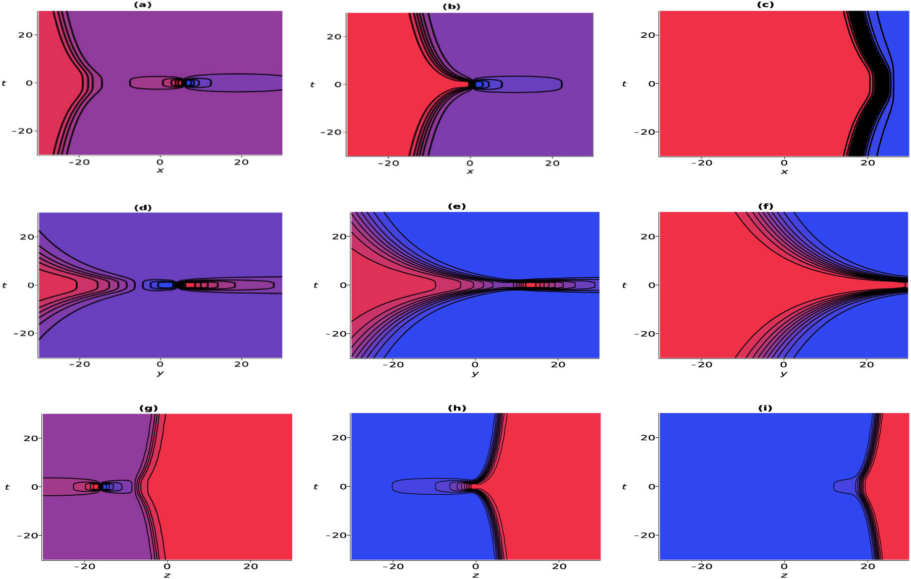
The contour propagation for the solution (10) with
3 Interaction solutions between stripe solitons and Jacobi elliptic function waves
This section is primarily concerned with the interaction between stripe solitons and Jacobi elliptic function waves. To this end, the function
where
where
By substituting Eq. (12) with Eqs. (13) into Eq. (3), the parameters can be obtained as follows:
from which the function
Then, the interaction solutions between stripe solitons and Jacobi elliptic function can be derived as follows:
Here, we take
Figure 2 presents the 3D evolution and density plots for the interaction solution (16) in the
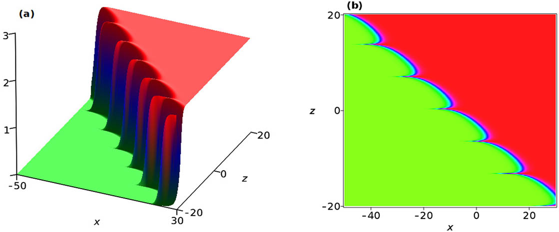
The evolution for the interaction solution (16) with parameters
4 Interaction solutions between lump and Jacobi elliptic function waves
The objective of this section is to obtain the interaction solutions between lump and Jacobi elliptic function waves for the HSIl Eq. (3). Here, we mainly give two construction methods.
Case 1
In this case, the function
with
where
By substituting function
from which the function
Then, the interaction between the lump and Jacobi elliptic function waves for the HSIl Eq. (3) can be given as follows:
where
It is obvious that the nonsingularity of solution (22) can be guaranteed by taking suitable values for the parameters
To demonstrate the evolution and interaction properties of the solution (22), we take parameters
which clearly has no singularity under condition

The 3D and contour propagation for the interaction solution (24) with parameters
Case 2
In this case, the function
with
where
where
from which the interaction solution between lump and Jacobi elliptic function waves for Eq. (3) can be obtained by substituting Eq. (28) into
Figure 4 shows the interaction process between the lump and Jacobi elliptic function waves at different times. It can be observed that as time
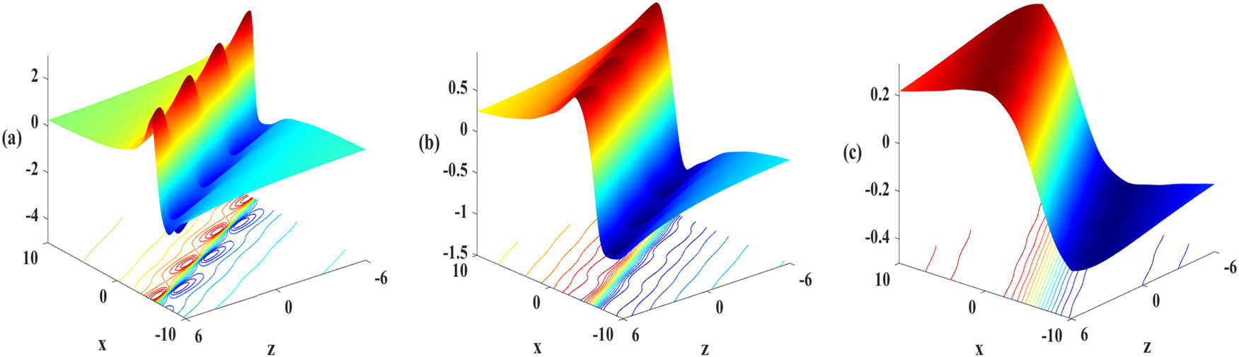
The 3D and contour propagation for the interaction solution (29) with parameters
5 Mixed interaction solutions
In this section, we attempt to construct the mixed interaction solutions combined with Jacobian, exponential, and integral quadratic functions. To this end, the function
with
where
By substituting Eq. (30) for Eq. (3), we have
where
Similar to the previous cases, the mixed solution

The 3D and contour propagation for the interaction solution (34) with parameters
In contrast to the case 2 figure presented in Section 4, Figure 5 depicts the presence of an additional striped soliton, which is more readily discernible from the expression of function
6 Conclusion and discussion
The present article examines the interactions between three distinct types of solutions, namely, lump, stripe solitons, and Jacobi elliptic function solutions. The (3+1)-dimensional HSIL equation has been constructed based on a modified direct method, with an accompanying discussion of its associated evolution and dynamics. In contrast to the independent variables of existing methods, which are typically represented by linear functions of spatial and temporal variables, the variables in this study represent a combination of linear functions of spatial variables and arbitrary spatial functions, thereby exhibiting a more intricate relationship with the dependent variables. As a result, a number of fascinating dynamical properties of the interaction solutions for the HSIl equation have been identified, which may provide theoretical insight into the underlying mechanisms of related nonlinear physical phenomena.
The study of interaction solutions enriches the structure of nonlinear local wave solutions for soliton equations, provides theoretical models for characterizing complex nonlinear phenomena in different physical fields, including nonlinear optics, plasma and oceanography, and provides theoretical guidance for predicting new nonlinear phenomena and designing new physical experiments. At the same time, it provides an information source for studying complex nonlinear waves using numerical simulation and deep learning method. Of course, there are still many issues that need further investigation, such as how to improve this method to obtain more physically meaningful interaction solutions and nonlinear dynamical properties? How to extend this method to more nonlinear evolution equations with practical physical significance? How to effectively combine numerical simulation and deep learning method to study the nonlinear dynamics of the interaction solutions in depth? These are also our upcoming studies in the near future.
Acknowledgments
This work was supported by the National Natural Science Foundation of China (Nos. 12075208 and 12171433).
-
Funding information: The authors state no funding involved.
-
Author contributions: Methodology: Xiaotian Liu; software: Xiaotian Liu; writing-original draft: Xiaotian Liu; writing-review and editing: Yunqing Yang; visualization: Xiaotian Liu and Yongshuai Zhang; supervision: Yongshuai Zhang and Yunqing Yang. All authors have accepted responsibility for the entire content of this manuscript and approved its submission.
-
Conflict of interest: The authors state no conflict of interest.
-
Data availability statement: All data generated or analysed during this study are included in this published article.
References
[1] Pitaevskii L, Stringari S. Bose–Einstein condensation and superfluidity. Oxford: Oxford University Press; 2016. 10.1093/acprof:oso/9780198758884.001.0001Search in Google Scholar
[2] Malomed BA. Nonlinear optics: symmetry breaking in laser cavities. Nat Photonics. 2015;9(5):287–9. 10.1038/nphoton.2015.66Search in Google Scholar
[3] Huchet M, Babarit A, Ducrozet G, Ferrant P, Gilloteaux JC, Droniou E. Experimental assessment of a nonlinear, deterministic sea wave prediction method using instantaneous velocity profiles. Ocean Eng. 2023;281:114739. 10.1016/j.oceaneng.2023.114739Search in Google Scholar
[4] Zabolotnykh AA. Nonlinear Schrödinger equation for a two-dimensional plasma: Solitons, breathers, and plane wave stability. Phys Rev B. 2023;108(11):115424. 10.1103/PhysRevB.108.115424Search in Google Scholar
[5] Yan ZY. Vector financial rogue waves. Phys Lett A. 2011;375(48):4274–9. 10.1016/j.physleta.2011.09.026Search in Google Scholar
[6] Hirota R. Direct methods in soliton theory. Berlin: Springer; 2004. 10.1017/CBO9780511543043Search in Google Scholar
[7] Matveev VB, Salle MA. Darboux transformation and solitons. Berlin: Springer-Verlag; 1991. 10.1007/978-3-662-00922-2Search in Google Scholar
[8] Ablowitz MJ, Clarkson PA. Solitons; nonlinear evolution equations and inverse scattering. Cambridge: Cambridge University Press; 1991. 10.1017/CBO9780511623998Search in Google Scholar
[9] Yang YL, Fan EG. Riemann–Hilbert approach to the modified nonlinear Schrödinger equation with non-vanishing asymptotic boundary conditions. Phys D. 2021;417:132811. 10.1016/j.physd.2020.132811Search in Google Scholar
[10] Raissi M, Perdikaris P, Karniadakis GE. Physics-informed neural networks: A deep learning framework for solving forward and inverse problems involving nonlinear partial differential equations. J Comput Phys. 2019;378:686–707. 10.1016/j.jcp.2018.10.045Search in Google Scholar
[11] Lin SN, Chen Y. Physics-informed neural network methods based on Miura transformations and discovery of new localized wave solutions. Phys D. 2023;445:133629. 10.1016/j.physd.2022.133629Search in Google Scholar
[12] Zhou ZJ, Yan ZY. Is the neural tangent kernel of PINNs deep learning general partial differential equations always convergent?. Phys D. 2024;457:133987. 10.1016/j.physd.2023.133987Search in Google Scholar
[13] Ullah N, Asjad MI, Rehman HU, A Akgül. Construction of optical solitons of Radhakrishnan-Kundu-Lakshmanan equation in birefringent fibers. Nonlinear Eng. 2022;11(1):80–91. 10.1515/nleng-2022-0010Search in Google Scholar
[14] Faridi WA, Asghar U, Asjad MI, Zidan AM, Eldin SM. Explicit propagating electrostatic potential waves formation and dynamical assessment of generalized Kadomtsev-Petviashvili modified equal width-Burgers model with sensitivity and modulation instability gain spectrum visualization. Results Phys. 2023;44:106167. 10.1016/j.rinp.2022.106167Search in Google Scholar
[15] Sagher AA, Asjad MI, Muhammad T. Advanced techniques for analyzing solitary waves in circular rods: a sensitivity visualization study. Opt Quant Electron. 2024;56:1673. 10.1007/s11082-024-07573-3Search in Google Scholar
[16] Strunin DV, Malomed BA. Symmetry-breaking transitions in quiescent and moving solitons in fractional couplers. Phys Rev E. 2023;107(6):064203. 10.1103/PhysRevE.107.064203Search in Google Scholar PubMed
[17] Rehman HU, Inc M, Asjad M, Habib A, Munir Q. New soliton solutions for the space-time fractional modified third order Korteweg-de Vries equation. J Ocean Eng Sci. 2022. 10.1016/j.joes.2022.05.032.Search in Google Scholar
[18] Asjad MI, Faridi WA, Alhazmi SE, Hussanan A. The modulation instability analysis and generalized fractional propagating patterns of the Peyrard-Bishop DNA dynamical equation. Opt Quant Electron. 2023;55:232. 10.1007/s11082-022-04477-ySearch in Google Scholar
[19] Liu M, Wang H, Yang H, Liu W. Study on propagation properties of fractional soliton in the inhomogeneous fiber with higher-order effects. Nonlinear Dyn. 2024;112:1327–37. 10.1007/s11071-023-09099-xSearch in Google Scholar
[20] Ma WX. Lump solutions to the Kadomtsev-Petviashvili equation. Phys Lett A. 2015;379(36):1975–8. 10.1016/j.physleta.2015.06.061Search in Google Scholar
[21] Ma WX. Interaction solutions to Hirota–Satsuma–Ito equation in (2+1)-dimensions. Front Math China. 2019;14:619–29. 10.1007/s11464-019-0771-ySearch in Google Scholar
[22] Wazwaz AM. Painlevé integrability and lump solutions for two extended (3+1)-and (2+1)-dimensional Kadomtsev-Petviashvili equations. Nonlinear Dyn. 2023;111:3623–32. 10.1007/s11071-022-08074-2Search in Google Scholar
[23] Wazwaz AM, Alhejaili W, El-Tantawy SA. On the Painlevé integrability and nonlinear structures to a (3+1)-dimensional Boussinesq-type equation in fluid mediums: Lumps and multiple soliton/shock solutions. Phys Fluids. 2024;36:033116. 10.1063/5.0194071Search in Google Scholar
[24] Zhang XE, Chen Y, Tang XY. Rogue wave and a pair of resonance stripe solitons to KP equation. Comput Math Appl. 2018;76(8):1938–49. 10.1016/j.camwa.2018.07.040Search in Google Scholar
[25] Chen ST, Ma WX. Lump solutions of a generalized Calogero-Bogoyavlenskii-Schiff equation. Comput Math Appl. 2018;76(7):1680–5. 10.1016/j.camwa.2018.07.019Search in Google Scholar
[26] Huang LL, Chen Y. Lump solutions and interaction phenomenon for (2+1)-dimensional Sawada-Kotera equation. Commun Theor Phys. 2017;67:473–8. 10.1088/0253-6102/67/5/473Search in Google Scholar
[27] Zhang XE, Chen Y. Rogue wave and a pair of resonance stripe solitons to a reduced (3+1)-dimensional Jimbo-Miwa equation. Commun Nonlinear Sci Numer Simul. 2017;52:24–31. 10.1016/j.cnsns.2017.03.021Search in Google Scholar
[28] Hirota R, Satsuma J. N-soliton solutions of model equations for shallow water waves. J Phys Soc Jpn. 1976;40(2):611–2. 10.1143/JPSJ.40.611Search in Google Scholar
[29] Zhou Y, Manukure S, Ma WX. Lump and lump soliton solutions to the Hirota–Satsuma–Ito equation. Commun Nonlinear Sci Numer Simul. 2019;68:56–62. 10.1016/j.cnsns.2018.07.038Search in Google Scholar
[30] Chen SJ, Ma WX, Lu X. Baaacklund transformation, exact solutions and interaction behaviour of the (3+1)-dimensional Hirota–Satsuma–Ito-like equation. Commun Nonlinear Sci Numer Simul. 2020;83:105–35. 10.1016/j.cnsns.2019.105135Search in Google Scholar
[31] Wang B, Ma Z, Liu X. Dynamics of nonlinear wave and interaction phenomenon in the (3+1)-dimensional Hirota–Satsuma–Ito-like equation. Eur Phys J D. 2022;76:165. 10.1140/epjd/s10053-022-00493-5Search in Google Scholar
[32] Liu S, Yang Z, Althobaiti A, Wang Y. Lump solution and lump-type solution to a class of water wave equation. Results Phys. 2023;45:106221. 10.1016/j.rinp.2023.106221Search in Google Scholar
[33] Liu JG, Eslami M, Rezazadeh H, Mirzazadeh M. Rational solutions and lump solutions to a non-isospectral and generalized variable-coefficient Kadomtsev-Petviashvili equation. Nonlinear Dyn. 2019;95:1027–33. 10.1007/s11071-018-4612-4Search in Google Scholar
[34] Ablowitz M, Satsuma J. Solitons and rational solutions of nonlinear evolution equations. J Math Phys. 1978;19(10):2180–6. 10.1063/1.523550Search in Google Scholar
© 2025 the author(s), published by De Gruyter
This work is licensed under the Creative Commons Attribution 4.0 International License.
Articles in the same Issue
- Research Articles
- Single-step fabrication of Ag2S/poly-2-mercaptoaniline nanoribbon photocathodes for green hydrogen generation from artificial and natural red-sea water
- Abundant new interaction solutions and nonlinear dynamics for the (3+1)-dimensional Hirota–Satsuma–Ito-like equation
- A novel gold and SiO2 material based planar 5-element high HPBW end-fire antenna array for 300 GHz applications
- Explicit exact solutions and bifurcation analysis for the mZK equation with truncated M-fractional derivatives utilizing two reliable methods
- Optical and laser damage resistance: Role of periodic cylindrical surfaces
- Numerical study of flow and heat transfer in the air-side metal foam partially filled channels of panel-type radiator under forced convection
- Water-based hybrid nanofluid flow containing CNT nanoparticles over an extending surface with velocity slips, thermal convective, and zero-mass flux conditions
- Dynamical wave structures for some diffusion--reaction equations with quadratic and quartic nonlinearities
- Solving an isotropic grey matter tumour model via a heat transfer equation
- Study on the penetration protection of a fiber-reinforced composite structure with CNTs/GFP clip STF/3DKevlar
- Influence of Hall current and acoustic pressure on nanostructured DPL thermoelastic plates under ramp heating in a double-temperature model
- Applications of the Belousov–Zhabotinsky reaction–diffusion system: Analytical and numerical approaches
- AC electroosmotic flow of Maxwell fluid in a pH-regulated parallel-plate silica nanochannel
- Interpreting optical effects with relativistic transformations adopting one-way synchronization to conserve simultaneity and space–time continuity
- Modeling and analysis of quantum communication channel in airborne platforms with boundary layer effects
- Theoretical and numerical investigation of a memristor system with a piecewise memductance under fractal–fractional derivatives
- Tuning the structure and electro-optical properties of α-Cr2O3 films by heat treatment/La doping for optoelectronic applications
- High-speed multi-spectral explosion temperature measurement using golden-section accelerated Pearson correlation algorithm
- Dynamic behavior and modulation instability of the generalized coupled fractional nonlinear Helmholtz equation with cubic–quintic term
- Study on the duration of laser-induced air plasma flash near thin film surface
- Exploring the dynamics of fractional-order nonlinear dispersive wave system through homotopy technique
- The mechanism of carbon monoxide fluorescence inside a femtosecond laser-induced plasma
- Numerical solution of a nonconstant coefficient advection diffusion equation in an irregular domain and analyses of numerical dispersion and dissipation
- Numerical examination of the chemically reactive MHD flow of hybrid nanofluids over a two-dimensional stretching surface with the Cattaneo–Christov model and slip conditions
- Impacts of sinusoidal heat flux and embraced heated rectangular cavity on natural convection within a square enclosure partially filled with porous medium and Casson-hybrid nanofluid
- Stability analysis of unsteady ternary nanofluid flow past a stretching/shrinking wedge
- Solitonic wave solutions of a Hamiltonian nonlinear atom chain model through the Hirota bilinear transformation method
- Bilinear form and soltion solutions for (3+1)-dimensional negative-order KdV-CBS equation
- Solitary chirp pulses and soliton control for variable coefficients cubic–quintic nonlinear Schrödinger equation in nonuniform management system
- Influence of decaying heat source and temperature-dependent thermal conductivity on photo-hydro-elasto semiconductor media
- Dissipative disorder optimization in the radiative thin film flow of partially ionized non-Newtonian hybrid nanofluid with second-order slip condition
- Bifurcation, chaotic behavior, and traveling wave solutions for the fractional (4+1)-dimensional Davey–Stewartson–Kadomtsev–Petviashvili model
- New investigation on soliton solutions of two nonlinear PDEs in mathematical physics with a dynamical property: Bifurcation analysis
- Mathematical analysis of nanoparticle type and volume fraction on heat transfer efficiency of nanofluids
- Creation of single-wing Lorenz-like attractors via a ten-ninths-degree term
- Optical soliton solutions, bifurcation analysis, chaotic behaviors of nonlinear Schrödinger equation and modulation instability in optical fiber
- Chaotic dynamics and some solutions for the (n + 1)-dimensional modified Zakharov–Kuznetsov equation in plasma physics
- Fractal formation and chaotic soliton phenomena in nonlinear conformable Heisenberg ferromagnetic spin chain equation
- Single-step fabrication of Mn(iv) oxide-Mn(ii) sulfide/poly-2-mercaptoaniline porous network nanocomposite for pseudo-supercapacitors and charge storage
- Novel constructed dynamical analytical solutions and conserved quantities of the new (2+1)-dimensional KdV model describing acoustic wave propagation
- Tavis–Cummings model in the presence of a deformed field and time-dependent coupling
- Spinning dynamics of stress-dependent viscosity of generalized Cross-nonlinear materials affected by gravitationally swirling disk
- Design and prediction of high optical density photovoltaic polymers using machine learning-DFT studies
- Robust control and preservation of quantum steering, nonlocality, and coherence in open atomic systems
- Coating thickness and process efficiency of reverse roll coating using a magnetized hybrid nanomaterial flow
- Dynamic analysis, circuit realization, and its synchronization of a new chaotic hyperjerk system
- Decoherence of steerability and coherence dynamics induced by nonlinear qubit–cavity interactions
- Finite element analysis of turbulent thermal enhancement in grooved channels with flat- and plus-shaped fins
- Modulational instability and associated ion-acoustic modulated envelope solitons in a quantum plasma having ion beams
- Statistical inference of constant-stress partially accelerated life tests under type II generalized hybrid censored data from Burr III distribution
- On solutions of the Dirac equation for 1D hydrogenic atoms or ions
- Entropy optimization for chemically reactive magnetized unsteady thin film hybrid nanofluid flow on inclined surface subject to nonlinear mixed convection and variable temperature
- Stability analysis, circuit simulation, and color image encryption of a novel four-dimensional hyperchaotic model with hidden and self-excited attractors
- A high-accuracy exponential time integration scheme for the Darcy–Forchheimer Williamson fluid flow with temperature-dependent conductivity
- Novel analysis of fractional regularized long-wave equation in plasma dynamics
- Development of a photoelectrode based on a bismuth(iii) oxyiodide/intercalated iodide-poly(1H-pyrrole) rough spherical nanocomposite for green hydrogen generation
- Investigation of solar radiation effects on the energy performance of the (Al2O3–CuO–Cu)/H2O ternary nanofluidic system through a convectively heated cylinder
- Quantum resources for a system of two atoms interacting with a deformed field in the presence of intensity-dependent coupling
- Studying bifurcations and chaotic dynamics in the generalized hyperelastic-rod wave equation through Hamiltonian mechanics
- A new numerical technique for the solution of time-fractional nonlinear Klein–Gordon equation involving Atangana–Baleanu derivative using cubic B-spline functions
- Interaction solutions of high-order breathers and lumps for a (3+1)-dimensional conformable fractional potential-YTSF-like model
- Hydraulic fracturing radioactive source tracing technology based on hydraulic fracturing tracing mechanics model
- Numerical solution and stability analysis of non-Newtonian hybrid nanofluid flow subject to exponential heat source/sink over a Riga sheet
- Numerical investigation of mixed convection and viscous dissipation in couple stress nanofluid flow: A merged Adomian decomposition method and Mohand transform
- Effectual quintic B-spline functions for solving the time fractional coupled Boussinesq–Burgers equation arising in shallow water waves
- Analysis of MHD hybrid nanofluid flow over cone and wedge with exponential and thermal heat source and activation energy
- Solitons and travelling waves structure for M-fractional Kairat-II equation using three explicit methods
- Impact of nanoparticle shapes on the heat transfer properties of Cu and CuO nanofluids flowing over a stretching surface with slip effects: A computational study
- Computational simulation of heat transfer and nanofluid flow for two-sided lid-driven square cavity under the influence of magnetic field
- Irreversibility analysis of a bioconvective two-phase nanofluid in a Maxwell (non-Newtonian) flow induced by a rotating disk with thermal radiation
- Hydrodynamic and sensitivity analysis of a polymeric calendering process for non-Newtonian fluids with temperature-dependent viscosity
- Exploring the peakon solitons molecules and solitary wave structure to the nonlinear damped Kortewege–de Vries equation through efficient technique
- Modeling and heat transfer analysis of magnetized hybrid micropolar blood-based nanofluid flow in Darcy–Forchheimer porous stenosis narrow arteries
- Activation energy and cross-diffusion effects on 3D rotating nanofluid flow in a Darcy–Forchheimer porous medium with radiation and convective heating
- Insights into chemical reactions occurring in generalized nanomaterials due to spinning surface with melting constraints
- Influence of a magnetic field on double-porosity photo-thermoelastic materials under Lord–Shulman theory
- Soliton-like solutions for a nonlinear doubly dispersive equation in an elastic Murnaghan's rod via Hirota's bilinear method
- Analytical and numerical investigation of exact wave patterns and chaotic dynamics in the extended improved Boussinesq equation
- Nonclassical correlation dynamics of Heisenberg XYZ states with (x, y)-spin--orbit interaction, x-magnetic field, and intrinsic decoherence effects
- Exact traveling wave and soliton solutions for chemotaxis model and (3+1)-dimensional Boiti–Leon–Manna–Pempinelli equation
- Unveiling the transformative role of samarium in ZnO: Exploring structural and optical modifications for advanced functional applications
- On the derivation of solitary wave solutions for the time-fractional Rosenau equation through two analytical techniques
- Analyzing the role of length and radius of MWCNTs in a nanofluid flow influenced by variable thermal conductivity and viscosity considering Marangoni convection
- Advanced mathematical analysis of heat and mass transfer in oscillatory micropolar bio-nanofluid flows via peristaltic waves and electroosmotic effects
- Exact bound state solutions of the radial Schrödinger equation for the Coulomb potential by conformable Nikiforov–Uvarov approach
- Some anisotropic and perfect fluid plane symmetric solutions of Einstein's field equations using killing symmetries
- Nonlinear dynamics of the dissipative ion-acoustic solitary waves in anisotropic rotating magnetoplasmas
- Curves in multiplicative equiaffine plane
- Exact solution of the three-dimensional (3D) Z2 lattice gauge theory
- Propagation properties of Airyprime pulses in relaxing nonlinear media
- Symbolic computation: Analytical solutions and dynamics of a shallow water wave equation in coastal engineering
- Wave propagation in nonlocal piezo-photo-hygrothermoelastic semiconductors subjected to heat and moisture flux
- Comparative reaction dynamics in rotating nanofluid systems: Quartic and cubic kinetics under MHD influence
- Laplace transform technique and probabilistic analysis-based hypothesis testing in medical and engineering applications
- Physical properties of ternary chloro-perovskites KTCl3 (T = Ge, Al) for optoelectronic applications
- Gravitational length stretching: Curvature-induced modulation of quantum probability densities
- The search for the cosmological cold dark matter axion – A new refined narrow mass window and detection scheme
- A comparative study of quantum resources in bipartite Lipkin–Meshkov–Glick model under DM interaction and Zeeman splitting
- PbO-doped K2O–BaO–Al2O3–B2O3–TeO2-glasses: Mechanical and shielding efficacy
- Nanospherical arsenic(iii) oxoiodide/iodide-intercalated poly(N-methylpyrrole) composite synthesis for broad-spectrum optical detection
- Sine power Burr X distribution with estimation and applications in physics and other fields
- Numerical modeling of enhanced reactive oxygen plasma in pulsed laser deposition of metal oxide thin films
- Dynamical analyses and dispersive soliton solutions to the nonlinear fractional model in stratified fluids
- Computation of exact analytical soliton solutions and their dynamics in advanced optical system
- An innovative approximation concerning the diffusion and electrical conductivity tensor at critical altitudes within the F-region of ionospheric plasma at low latitudes
- An analytical investigation to the (3+1)-dimensional Yu–Toda–Sassa–Fukuyama equation with dynamical analysis: Bifurcation
- Swirling-annular-flow-induced instability of a micro shell considering Knudsen number and viscosity effects
- Numerical analysis of non-similar convection flows of a two-phase nanofluid past a semi-infinite vertical plate with thermal radiation
- MgO NPs reinforced PCL/PVC nanocomposite films with enhanced UV shielding and thermal stability for packaging applications
- Optimal conditions for indoor air purification using non-thermal Corona discharge electrostatic precipitator
- Investigation of thermal conductivity and Raman spectra for HfAlB, TaAlB, and WAlB based on first-principles calculations
- Tunable double plasmon-induced transparency based on monolayer patterned graphene metamaterial
- DSC: depth data quality optimization framework for RGBD camouflaged object detection
- A new family of Poisson-exponential distributions with applications to cancer data and glass fiber reliability
- Numerical investigation of couple stress under slip conditions via modified Adomian decomposition method
- Monitoring plateau lake area changes in Yunnan province, southwestern China using medium-resolution remote sensing imagery: applicability of water indices and environmental dependencies
- Heterodyne interferometric fiber-optic gyroscope
- Exact solutions of Einstein’s field equations via homothetic symmetries of non-static plane symmetric spacetime
- A widespread study of discrete entropic model and its distribution along with fluctuations of energy
- Empirical model integration for accurate charge carrier mobility simulation in silicon MOSFETs
- The influence of scattering correction effect based on optical path distribution on CO2 retrieval
- Anisotropic dissociation and spectral response of 1-Bromo-4-chlorobenzene under static directional electric fields
- Role of tungsten oxide (WO3) on thermal and optical properties of smart polymer composites
- Analysis of iterative deblurring: no explicit noise
- The influence of anisotropy of InP on its elasticity and phonon properties
- Review Article
- Examination of the gamma radiation shielding properties of different clay and sand materials in the Adrar region
- Erratum
- Erratum to “On Soliton structures in optical fiber communications with Kundu–Mukherjee–Naskar model (Open Physics 2021;19:679–682)”
- Special Issue on Fundamental Physics from Atoms to Cosmos - Part II
- Possible explanation for the neutron lifetime puzzle
- Special Issue on Nanomaterial utilization and structural optimization - Part III
- Numerical investigation on fluid-thermal-electric performance of a thermoelectric-integrated helically coiled tube heat exchanger for coal mine air cooling
- Special Issue on Nonlinear Dynamics and Chaos in Physical Systems
- Analysis of the fractional relativistic isothermal gas sphere with application to neutron stars
- Abundant wave symmetries in the (3+1)-dimensional Chafee–Infante equation through the Hirota bilinear transformation technique
- Successive midpoint method for fractional differential equations with nonlocal kernels: Error analysis, stability, and applications
- Novel exact solitons to the fractional modified mixed-Korteweg--de Vries model with a stability analysis