Abundant wave symmetries in the (3+1)-dimensional Chafee–Infante equation through the Hirota bilinear transformation technique

1 Introduction

Solitons are solitary waves (or self-reinforcing waveforms) that travel at a constant speed, keeping their shape in the way. They form the core of nonlinear science, and they result from the balance of nonlinearity and dispersion. As a consequence, they are critical to understanding several fundamental physical and mathematical systems. Solitons abound in most fields, such as fluid [1], plasma physics [2], optical communication [3], stellar environments [4], and biology [5], to mention only a few. Among many equations modeling the behavior of solitons, such as the nonlinear chains of atoms model [6], the bistable Allen-Cahn equation [7], and the coupled nonlinear Schrüdinger-type equations [8], as well as the ( 3 + 1 ) -dimensional Calogero–Bogoyavlenskii–Schiff (CBS) equation, the CBS–Bogoyavlensky–Konopelchenko (CBS-BK) equation [9], the unstable NLSE and the modify unstable NLSE [10], and so on, the Chafee–Infante equation (CIE) can rightly be classified as a celebrated reaction–diffusion model [11]. This equation describes the energy balance between equator and pole of the solar system, which transmit energy via heat diffusion [12].

The one-dimensional CIE has emerged as one important topic of mathematical research. This equation has been analyzed with the sole aim of discovering its attractor structure and developing various stability characteristics [13]. For example, Caraballo et al. [14] shed light on the effects of stochastic perturbations on this equation through their investigations, which led to an intriguing conclusion on the noise and system synthesis. Such investigations showed how multiplicative Itô noise could stabilize the origin, while Stratonovich noise preserved the attractor’s dimension. They also showed that sufficiently rich additive noise could reduce the random attractor to a single point. They also emphasized the importance of noise in modulating the dynamics of reaction–diffusion systems. In turn, Debussche et al. [15] addressed thoroughly the deterministic CIE with special reference to its long-time dynamics and attractor structures. Their work showed how stable and unstable manifolds direct solutions toward equilibrium. The initial results formed a basis for future research efforts concerning the equation’s response to perturbations and modification of parameters.

Undoubtedly, the CIE has been extended from the one-dimensional case into higher-dimensional transitions. An application of the equation to mass transport, particle diffusion, and energy transfer has been made for two and three spatial dimensions. Rosa [16] applied the inertial manifold theory in designing exact finite-dimensional feedback control laws for the equation to demonstrate its potential in control theory. The investigation highlighted the capacity of the CIE as a model for the controlled nonlinear systems. As a follow-up, Carvalho et al. [17] studied the nonautonomous version of the equation, providing a detailed analysis of its pullback attractor structure and the bifurcations that arise when parameters are varied. Such works are examples of dynamic behavior captured with this versatile equation in various settings. In addition, stochastic modifications of the CIE have also attracted much interest. Blumenthal [18] investigated pitchfork bifurcations in the face of stochastics and found that, even with the destruction of random pullbacks, finite-time Lyapunov exponents persist. The contribution provides new prospects the regarding bifurcation theory in stochastic systems by demonstrating that noise acts to simultaneously destabilize and preserve important dynamical features.

On the other hand, analytical techniques have played a very vital role in exploring the solutions and properties of the CIE. For example, using the modified F-expansion method, Tang and Wang [19] derive bright and kink soliton solutions and provide stability analyses of their behavior. Hossain et al. [20] have contributed to this work by incorporating conformable fractional derivatives into this equation and discovering multisoliton interactions and waveforms in trigonometric, hyperbolic, and exponential forms by applying the nonlinear M-shaped expansion method. More work has been done concerning novel solutions of the CIE. Rached [21] used the enhanced modified simple equation method to construct exact solutions and extend the range of analytical solutions known until now. Mahmood et al. [22] presented the modified Khater method for solving the (2+1)-dimensional version of the equation that describes a wide variety of propagating wave patterns, including bright and dark solitons, as well as periodic solitons. Arshed et al. [23] employed this equation to gain soliton solutions in hyperbolic, trigonometric, and rational form with the extended G ′ G 2 -expansion method and new F G -expansion method. The applicability of the equation was further highlighted for phenomena in fluid-dynamics, plasma physics, and nonlinear optical systems. They stressed the role of conservation laws in understanding the integrability of the equation.

Furthermore, Arshed et al. [24] hastened the study of this equation by finding solutions such as bright, dark, periodic, kink, anti-kink, and singular traveling wave patterns with the extended sinh-Gordon equation expansion technique. Kumar et al. [25] employed the generalized exponential rational function (GERF) technique to derive quite a number of soliton solutions to the (2+1)-dimensional CIE. Their work yielded closed-form solutions in the form of bright soliton and dark solitons, combined and singular profiles, periodic oscillatory waves, and kink-wave structures. Akbar et al. [26] used first integral method to realize solitary wave solution for NLEEs such as CIE. They showed how the solutions obtained can be used in physical applications. Also, Cimpoiasu [27] put forth an introduction of a modified auxiliary equation (MAE) method associated with stochastic differential equations for soliton solution investigation of the CIE. This new method uses stochastic processes such as Wiener process to study magnitude and behavior of solitons under their stochastic influences. Their work brought in new insights into the stochastic dynamics of solitons and helps for understanding soliton behavior against random perturbations. Khater and Ghanbari [28] also employed the generalized expansion method to solve this equation under time-variable coefficients. Such an approach included nonlinear wave variables along with auxiliary equations such as Riccati equations and Jacobian elliptic equations to present nonautonomous solutions formed by triangular, rational, or doubly-periodic structures showing the effect of variable coefficients on the performance of solitons.

It is worth noting that the studies mentioned earlier were all based on either ( 1 + 1 ) or ( 2 + 1 ) -dimensions. From the literature, one of the few works on the ( 3 + 1 ) -dimensional CIE are those by Sebogodi et al. [29], who derived soliton solutions using methods such as GERF, first integral, and expansion techniques. Likewise, Khater and Alfalq [30] employed the fractional nonlinear generalized ( 3 + 1 ) -dimensional CIE to model wave propagation in dispersive media. However, these include analytical and numerical solutions that demonstrate that wave dynamics were simulated efficiently using the Khat II and He’s variational iteration method. Collectively, these works speak of the multifunctional character of the equation as a model of nonlinear systems. The results embody the efforts to create and sustain high-level computations for the interpretation of analytical solutions. The generalized (3+1)-dimensional CIE provides an important ground to harvest nonlinear wave dynamics in multidimensional systems. This equation is formulated in the form [29]

where N ( x , y , z , t ) represents the wave function in the entering parameters a , b , c , and d , which govern the nonlinearity and dispersion as well as the reaction–diffusion effects. Also, higher dimensional terms make this equation a candidate for very complex interactions, like in the case of high energy physical processes, environmental systems, or optical waveguides. The model is an essential generalization of the reaction–diffusion model, where extra spatial directions are added to explain intricate wave behavior in systems of higher dimension. The model has important implications in nonlinear optics for explaining propagation of ultrashort pulses through multimode fibers, in plasma physics for understanding ion-acoustic waves in magnetized plasmas, and in fluid mechanics for studying formation of rogue waves in three-dimensional oceanic domains. The inclusion of multiple spatial dimensions ( y , z ) enables cross-directional wave interaction and pattern formation to be examined, making it especially applicable for the understanding of energy transport in anisotropic media. In the quantum field theory, it can be used as a model for the investigation of spontaneous symmetry breaking in ( 3 + 1 ) -dimensional systems. The nonlinear terms of the model account for key aspects of wave self-focusing and modulation instability, while its dispersive terms explain wave broadening effects, making it important in predicting extreme wave events in natural and engineered systems. Recent uses include biophysics to model signal propagation in three-dimensional neural networks and materials science to analyze nonlinear elastic waves in crystalline materials. The versatility of the equation to accommodate various solution types (solitons, breathers, rogue waves) under various parameter regimes renders it a valuable instrument for exploring nonlinear wave phenomena across various disciplines.

The Hirota bilinear transformation technique has proven to be a very capable device both for the solving of nonlinear partial differential equations and the discovery of different forms of wave phenomena, such as solitons, breathers, lumps, M-shaped, periodic, kink, and rogue waves. By demonstrating the versatility of this technique, Yin et al. [31] took this procedure into ( 3 + 1 ) -dimensional equations to facilitate rational transformations for deriving complex solutions of generalized shallow water wave equations that present rogue waves and interaction solutions. Furthermore, Li et al. [32] proposed an extended Hirota’s method developing modification rules in summation to reveal more complicated structures as M -shaped, molecular, or web-like solitons in the (2+1) Sawada-Kotera equation and much more. These improvements highlight the flexibility of the method to give suitable treatment for complex wave motions within a variety of dimensions and contexts. More researchers delve into real-life application and computational techniques for Hirota’s method. However Yokus and Isah [33] go a step further and combine it with a new exponential function technique to study sections of KdV solutions about soliton stability and nonlinear wave interaction. Zhang et al. [34] considered shock wave responses of equations of type KdV–Burgers and Zakharov–Kuznetsov–Burgers and tried to relate them to dissipation effects with physical wave behavior. According to Ceesay et al. [35] about M -soliton solutions of the modified regularized long wave equation, these reflect real life in terms of coastal dynamics with possible insights into sediment transport and erosion effects. Kumar and Mohan [36] on the hand gain multi-soliton solutions to high-dimensional equations using this method. Ahmad et al. [37] applied to nonlocal KdV equations and came out with bright soliton solutions with some interesting features. By using the Hirota bilinear transformation technique, Gu et al. [38] analyzed the (2+1)-dimensional Kadomtsev–Petviashvili–Sawada–Kotera–Ramani (KPSKR) equation, obtaining its soliton, breather, and lump solutions, and explore their interactions along with the concerned chaotic dynamics of the model. In a similar work, Gu et al. [39] also explore the (3+1)-dimensional Kadomtsev–Petviashvili–Boussinesq-like equation employing the same approach to derive soliton, lump, and traveling wave solutions as well as exploring the model’s chaotic behavior. Shehzad et al. [40] used the Hirota bilinear method for a wider set of nonlinear wave structures such as lump, rogue, breather, and periodic waves, with focus on their interactions and physical importance in plasma systems, ocean wave dynamics, and other realistic applications. These works and numerous others prove the profound effect that the Hirota bilinear method has on mathematical physics, applied sciences, and the changing of theoretical insights into the practical domain.

Despite significant advances in studying the CIE in lower dimensions, not much work has been done investigating its (3+1)-dimensional version using the Hirota bilinear transformation method. This research fills that void by deriving a wide range of exact wave solutions such as bright and dark solitons, breathers, lumps, M-shaped waves, and periodic cross kink waves within this higher dimensional context. The novelty of this work lies in the rigorous application of Hirota’s technique for deriving and visualizing intricate wave interactions that are still analytically manageable but dynamically complex. These results not only deepen the theory of soliton dynamics in multidimensional systems but also expand the applicability of the CIE to nonlinear waves in physics and engineering. Hence, this work enhances the study of nonlinear wave analysis and provides a solid base for further theoretical research and applications in real-life situations concerning multidimensional soliton phenomena.

The rest of this article is structured as follows. In Section 2, the Hirota bilinear approach is briefly reviewed, and the bilinear form of the (3+1)-dimensional CIE is established. We also exhibits a set of exact solutions for this model. In Section 3, we highlight the graphical representations and a detailed analysis of the dynamical behavior of these solutions. Section 4 shows the results comparison of the manuscript, and Section 5 ends the article by summarizing main findings and possible areas of the future work.

2 The Hirota bilinear method

The Hirota bilinear technique is a popular and powerful analytical method for determining exact solutions of nonlinear partial differential equations (NLPDEs). Its main advantage consists of being systematic and constructive in nature, enabling to derive soliton, lump, breather, and other interactive solutions without needing to linearize or approximate. The technique operates effectively by transforming the NLPDE into a bilinear form through dependent variable transformations so that the process of solution can be treated algebraically. Another benefit is that it can treat multisoliton and higher-dimensional solutions, and it is appropriate for the investigation of complex wave structures such as those in the (3+1)-dimensional CIE examined in this research. In addition, it allows one to build up solutions with controllable parameters for in-depth wave behavior, stability, and interactions analysis.

There are, however, some weaknesses in the approach. One is that it commonly depends on specific transformations and assumptions (e.g., exponential forms of the solutions), which are not necessary for all forms of nonlinear equations especially nonpolynomial or nonintegrable ones. Also, the approach does not deal with boundary or initial conditions directly, so its use is mainly within the framework of determining formal exact solutions but not complete boundary value problems. Moreover, although the bilinear form is compact, the algebra may grow more complicated when dealing with higher-order or generalized equations, necessitating the use of symbolic computation tools for effective application. In spite of these constraints, the Hirota method is still a very efficient and flexible method, particularly for researchers who wish to investigate the rich structure of nonlinear wave dynamics in both lower and higher dimensions.

We now proceed to use this method in Eq. (1). To do so, first, we make the Cole–Hopf transformation; that is, we take the logarithmic transformation of the dependent variable N , giving us the assumption that the solution to Eq. (1) is,

where R is a constant to be determine. To find R , we begin by using the following function:

where α i , β i , and λ i represent the wave numbers, and ω i represents the dispersion. By putting Eq. (3) into the linear parts of Eq. (1), we obtain the dispersion relation as follows:

We now replace the function

into the Cole–Hopf transformation in Eq. (2), and by using the result in Eq. (1), we can solve for R to obtain

Therefore, the logarithmic transformation becomes

We transformed the linear terms of Eq. (1) into bilinear form as follows:

We would enter into Eq. (8) all forms of wave functions under study with means of Mathematica. Then for each specific case, we will expand and evaluate and arrange related terms as related to one another, setting them to 0. This will lead us to solutions of these systems of equations, finding various potential families corresponding to each case.

1. Interaction via double exponents: This wave structure is given in the following equation [41]:

   (9) k ( x , y , z , t ) = P 1 exp ( h ( L 1 ( t w + x + y + z ) + L 2 ) ) + P 2 exp ( h ( L 3 ( t w + x + y + z ) + L 4 ) ) .

Category 1: L 1 = 0 , L 3 = − i b 2 h , w = − 3 i b 2 − c − d . If we put them into Eq. (9) and inject the outcome into Eq. (7), we obtain the result as follows:

Category 2: L 1 = i b 2 h , L 3 = − i b 2 h , w = − c − d . If we put them into Eq. (9) and inject the outcome into Eq. (7), we obtain the result as follows:

1. Interaction of M-shaped rational wave with one kink: This wave configuration is provided in the following equation [41]:

   (12) k ( x , y , z , t ) = P 1 exp ( L 1 ( t w + x + y + z ) + L 2 ) + ( L 3 ( t w + x + y + z ) + L 4 ) 2 + ( L 5 ( t w + x + y + z ) + L 6 ) 2 + L 7 .

Category 1: L 1 = − i b 2 , L 3 = 0 , L 5 = 0 , w = − 3 i b 2 − c − d . By substituting them into Eq. (12) and then substituting the result into Eq. (7), we obtain

1. Interaction of M-shaped rational wave with rogue and kink: This wave configuration is provided in the following equation [41]:

Eq. (14) and its partial derivatives up to third order are substituted into Eq. (8), followed by simplification. The like terms are then collected so that for every expression, the coefficients of each expression set to zero. Thus, a category of constant values emerges from this system of equations:

Category 1: L 1 = − i b 2 , L 3 = − i b 2 , L 5 = − i L 7 , L 6 = 0 , L 8 = 0 , L 9 = 0 , w = − c − d . When we substitute these into Eq. (14) and insert the outcome into Eq. (7), we then end up with the result as follows:

1. Mixed waves: This wave configuration is provided in the following equation [42]:

   (16) k ( x , y , z , t ) = P 1 exp ( h ( L 1 ( t w + x + y + z ) + L 2 ) ) + P 2 exp ( − h ( L 1 ( t w + x + y + z ) + L 2 ) ) + P 3 sin ( h ( L 3 ( t w + x + y + z ) + L 4 ) ) + P 4 sinh ( h ( L 5 ( t w + x + y + z ) + L 6 ) ) .

Category 1: L 1 = − i b 2 h , L 3 = b 2 h , L 5 = − i b 2 h , w = − c − d . By inserting them into Eq. (16), and then the result into Eq. (7), we have

where

Category 2: P 2 = 0 , L 1 = i b 2 h , L 3 = b 2 h , L 5 = − i b 2 h , w = − c − d . If we substitute them into Eq. (16) and then that result into Eq. (7), we have

where

1. Multiwaves: This pattern of waves is offered in [42]

   (19) k ( x , y , z , t ) = P 2 cos ( L 3 ( t w + x + y + z ) + L 4 ) + P 1 cosh ( L 1 ( t w + x + y + z ) + L 2 ) + P 3 cosh ( L 5 ( t w + x + y + z ) + L 6 ) .

Category 1: P 3 = 0 , L 1 = i b 2 , L 3 = b 2 , w = − c − d . By plugging them into Eq. (19) and subsequently into Eq. (7), we obtain

1. Periodic lump: This wave structure is given in the following equation [43]:

   (21) k ( x , y , z , t ) = ( L 1 ( t w + x + y + z ) + L 2 ) 2 + ( L 3 ( t w + x + y + z ) + L 4 ) 2 + cos ( L 5 ( t w + x + y + z ) + L 6 ) + L 7 .

Category 1: L 1 = i L 3 , L 2 = 0 , L 4 = 0 , L 5 = b 2 , L 7 = 0 , w = − c − d . By placing them into Eq. (21) and the outcome into Eq. (7), we obtain the result as follows:

1. Periodic cross kink: This pattern of waves is offered in the following equation [43]:

   (23) k ( x , y , z , t ) = P 1 exp ( h ( L 3 ( t w + x + y + z ) + L 4 ) ) + exp ( h ( L 1 ( t w + x + y + z ) + L 2 ) ) + P 2 cos ( h ( L 5 ( t w + x + y + z ) + L 6 ) ) + P 3 cosh ( h ( L 7 ( t w + x + y + z ) + L 8 ) ) + L 9 .

Category 1: L 1 = i b 2 h , L 3 = i b 2 h , L 5 = − b 2 h , L 7 = − i b 2 h , L 9 = 0 , w = − c − d . By replacing these into Eq. (23) and then the result into Eq. (7), we obtain

where

Category 2: P 1 = 0 , L 1 = − i b 2 h , L 5 = − b 2 h , L 7 = − i b 2 h , L 9 = 0 , w = − c − d . By substituting them into Eq. (23) and then the result into Eq. (7), we have

where

1. Homoclinic breather: This form of waves is given in the following equation [44]:

   (26) k ( x , y , z , t ) = P 1 exp ( h ( L 1 ( t w + x + y + z ) + L 2 ) ) + P 2 exp ( − h ( L 3 ( t w + x + y + z ) + L 4 ) ) + P 3 cos ( h ( L 5 ( t w + x + y + z ) + L 6 ) ) .

   With the substitution of Eq. (26) and its first four partial derivatives into (8), and simplified. We then assemble and group together similar terms and equate zeroes to each one’s coefficient. Thus, we obtain the following categories of constant values: Category 1: L 1 = i L 5 , L 3 = i L 5 , w = − c − d , h = b 2 L 5 . By inserting these into Eq. (26) and then the result into Eq. (7), we obtain

   (27) N 1 H B ( x , y , z , t ) = i 3 b − F 9 + P 1 exp b ( − 2 i L 5 ( c t + d t − x − y − z ) + L 2 + L 4 ) 2 L 5 a F 10 + P 1 exp b ( − 2 i L 5 ( c t + d t − x − y − z ) + L 2 + L 4 ) 2 L 5 ,

   where

   F 9 = P 2 + i P 3 exp b ( L 4 + i L 5 ( − c t − d t + x + y + z ) ) 2 L 5 × sin b ( L 5 ( − c t − d t + x + y + z ) + L 6 ) 2 L 5 , F 10 = P 2 + P 3 exp b ( L 4 + i L 5 ( − c t − d t + x + y + z ) ) 2 L 5 × cos b ( L 5 ( − c t − d t + x + y + z ) + L 6 ) 2 L 5 .

   Category 2: P 1 = 0 , L 3 = − i L 5 , w = − c − d , h = b 2 L 5 . By exporting them into Eq. (26) and then the result into Eq. (7), we have

   (28) N 2 H B ( x , y , z , t ) = i 3 b P 2 + i P 3 exp b ( L 4 − i L 5 ( − c t − d t + x + y + z ) ) 2 L 5 sin b ( L 5 ( − c t − d t + x + y + z ) + L 6 ) 2 L 5 a P 2 + P 3 exp b ( L 4 − i L 5 ( − c t − d t + x + y + z ) ) 2 L 5 cos b ( L 5 ( − c t − d t + x + y + z ) + L 6 ) 2 L 5 .

3 Discussion

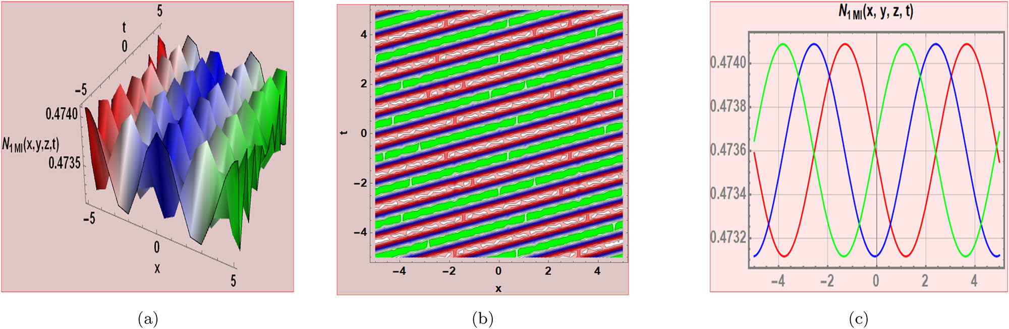
The 3D figures, their corresponding contours, and 2D plots for the obtained solutions are constructed using Mathematica and are displayed in Figures 1–12, which aid in the visualization of the solutions’ characteristics. The 3D surface plot in Figure 1(a) describes the event from the superposition of two exponentially propagating waves that yield a bright solitons, localized wave packets that keep their amplitude and shape while propagating along a certain medium. These solitons are formed as a balance of nonlinearity and dispersion in a single energetic and stable compact form, which is a property common for solitons in nonlinear systems such as shallow water waves and plasmas. The contour plot in Figure 1(b) shows how the soliton’s space changes as time progresses. This set of contours is able to visualize the translation of the wave along the x-axis at fixed amplitudes. In Figure 1(c), the 2D plot depicts the amplitude of the solitary wave at t = 0 (in red), t = 1 (in blue), and t = 2 (in green). This indicates that the solitary wave propagates without dispersion, an important feature of soliton dynamics. The 3D graph shown in Figure 2(a) describes wave interactions from two exponential functions demonstrating the interaction of two solitons as they coalescence and then again repulse each other with time, and represents dark solitons which are trough-like structures found within the wave profile. The significant property of soliton dynamics indicates that the solitons have an elastic collision, preserving the shape and velocity. The interaction itself shows the system’s nonlinearity and stability. The contour plot in Figure 2(b) shows dark soliton stability in space and time. The oscillating regions of high and low energy density indicate stable wave profiles with dark troughs retaining their positions. In Figure 2(c), the coexistence of dark solitons is depicted in the 2D plots – they are at different moments, with depth and all shapes remaining constant at t = 0 (red), t = 1 (blue), and t = 2 (green), showing a strong robustness and stable dynamics as well as showing how the amplitudes and structures are preserved after the collision. Profiles verify that the interaction is elastic, and no energy is lost during the process.

Figure 1

The 3D, contour, and 2D representations depict the interaction through a two-exponent type wave.

Figure 2

The 3D, contour, and 2D representations depict the interaction through a two-exponent type wave.

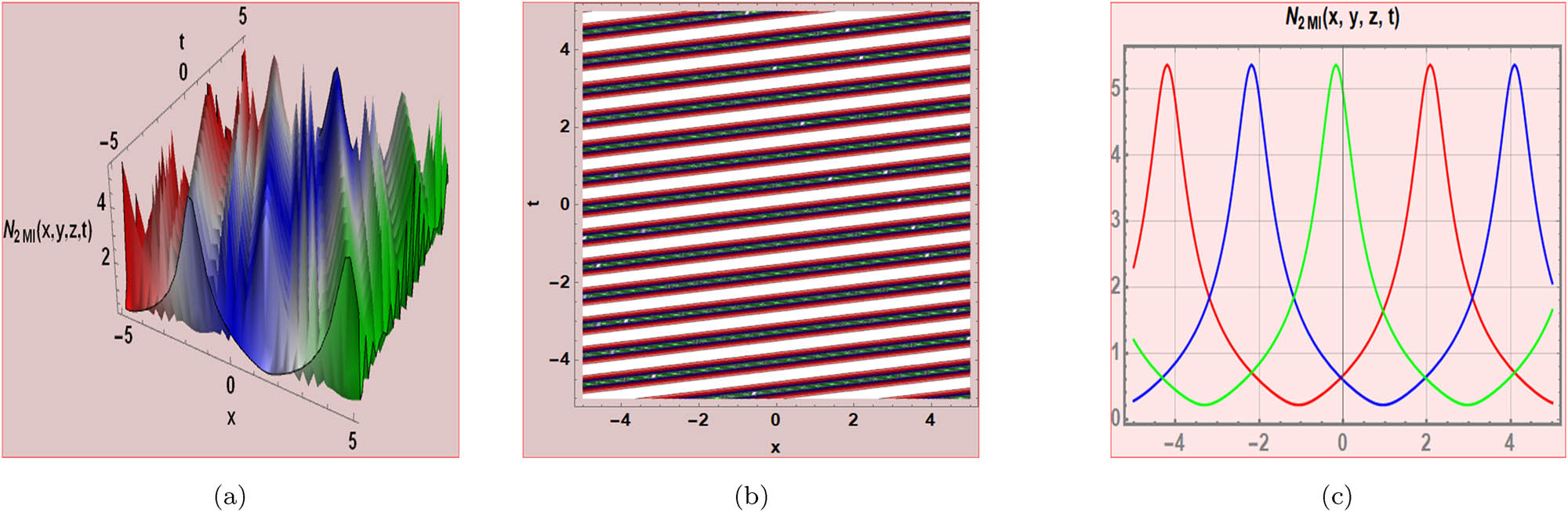
Figure 3(a) deals with a 3D plot obtained from an M-shaped wave interaction with single kink. It reveals a pronounced M-shaped wave with solely one side being kinked, with the M-shape propagating along the space domain over the time. The kink is a site-specific and abrupt transition in the amplitude of the wave, which may be associated with a nonlinear phenomenon. Such a wave is a traveling wave that bears localized perturbations that, in course of time, do not change their configuration. Figure 3(b) is a contour map showing the M-like structure propagating periodically along with the kink as a sudden and time-consistent discontinuity in phase across space and time. This implies that the system is dynamically stable living under a balance of dispersion and nonlinearity characteristics typical of, for instance, a solitonic wave. The 2D graph in Figure 3(c) shows the M-shaped wave profiles at varying time steps ( t = 0 ) red, ( t = 1 ) blue, and ( t = 2 ) green, and how the wave moves while keeping the spatial configuration intact. This is indicative of robustness under propagation, which seems to characterize nonlinear wave systems or traveling wave solutions. Figure 4(a) is a 3D plot showing a wave with an M-shape and acting with rogue and kink. The point of a double peak due to the nonlinear interaction effects. The peaks are symmetric, indicating the equilibrium between effects due to amplitude and dispersion. Figure 4(b) is a contour plot depicting the coherent propagation of M-shaped waves, which exhibit a perfect double-peak structure. An identical geometry of double peaks is thus a sign of their nonlinear stability in time and space. The 2D plots in Figure 4(c) illustrate the propagation of the M-shaped waves. They have the same symmetrical double peaks, which do not change for t = 0 (red), t = 1 (blue), and t = 2 (green) this confirms its persistence stability.

Figure 3

Shows the 3D, contour, and 2D graphs of an M-shaped rational wave containing a single kink.

Figure 4

Exhibits a 3D, contour, and 2D charts of an M-shaped rational wave interacting with rogue and kink.

The 3D illustration in Figure 5(a) is obtained from mixed waves structure. The mixed-frequency wave shows several modes oscillating, thus superimposing the waves as a representation of phenomena like wave interference. The contour plot of Figure 5(b) shows the superposed wave forms and in semblance to the structure of a grid, which indicates interaction between different wave frequencies or wavelengths; it may signify constructive and destructive interferences. As indicated in Figure 5(c), the 2D plots of wave amplitude for t = 0 (red), t = 1 (blue), and t = 2 (green). The profiles display the phase and amplitude shifts due to combined effects of waves signifying dynamic interference. The 3D graph of Figure 6(a) is gained from a mixed wave configuration. It shows oscillatory solitons that combine the two features of periodic wave forms as well as localized wave structures in their manifestation. Their motion suggests an equilibrium between the nonlinearity and dispersion, which results in that these repetitive states are always observed to be present even as they oscillate for long periods of time. The contour plot in Figure 6(b) captures the solitons repetitive and oscillatory features whereby the crests of the wave form traces a consistent shape revealing an indication that they propagate through time in a stable fashion with an overall periodic redistribution of energy. The 2D plot in Figure 6(c) indicates representation at t = 0 (red), t = 1 (blue), and t = 2 (green), showing how their movement is oscillatory. The amplitude periodically varies due to the contribution of the effects of focusing and defocusing. Figure 7(a) depicts the 3D plot that shows multi waves interacting. In fact, it show some periodic breather waves. Amplitude oscillation represents the energy exchanged within the system, a phenomenon typical of breather solutions. Figure 7(b) depicts contour plot corresponding to the periodical spatial distribution of the breather waves, confirming the evidence that they form a pattern and grants dynamism with the energy exchange and localization itself. The 2D plot is shown in Figure 7(c) illustrates the oscillatory behavior of the breather waves at t = 0 (red), t = 1 (blue), and t = 2 (green). The stable modulation is what affirms that the breather solution remains so through time.

Figure 5

The 3D, contour, and 2D diagrams are obtained from the mixed waves function.

Figure 6

The 3D, contour, and 2D diagrams are obtained from the mixed waves function.

Figure 7

Displays multiwave types’ 3D, contour, and 2D plots.

Figure 8(a) shows a periodic lump wave in a 3D plot that consists of a periodic arrangement of lumps in the spatial domain. Each lump exhibits the behavior of a solitary localized wave, similar to a typical lump wave and has an area of decay on either side from the center of each peak. The periodic structure in a lump wave configuration arises out of nonlinear interactions in the system that make it possible to obtain a stable repetitive configuration. Contour plot display in Figure 8(b) displays the time stable states of the multisolitons. Clearly defined peaks in them attest their coherent propagation. The 2D plot in Figure 8(c) present the formation and movement of multi-soliton waves. The t = 0 (red), t = 1 (blue), and t = 2 (green) profiles are distinct and stable, characteristic of the solitonic interaction. The 3D representation of a periodic cross-kink wave is shown in Figure 9(a). It captures repetitive periodicities of cross-kinks. Periodic overlap of structures indicates possible nonlinear interaction effects of wave propagation by kink-like waves propagating at different orientations. The contour plot of Figure 9(b) captures the cross-pattern of periodic distribution of the kinks, indicating stable propagation and periodic overlaps of the kink structures. The 2D plot of Figure 9(c) demonstrate the stability of cross-kinks. The coherent dynamics and robust structure of the periodic waveforms are shown at t = 0 (red), t = 1 (blue), and t = 2 (green). The 3D representation of a periodic cross-kink wave is shown in Figure 10(a). It flexes the traveling solitons periodically with a train structure. These solitons maintain their amplitude and phase during propagation uniformly in the medium. It reflects soliton stability and periodicity in the wave system. The contour plot of Figure 10(b) captures its periodic nature with equally spaced and uniform stripes of solitons. Such patterns show the coherent propagation of solitons without any amplitude decay and with minimal interaction. The 2D plot of Figure 10(c) with varying time at t = 0 (red), t = 1 (blue), and t = 2 (green) shows the solitons keeping their amplitude and the wavelength remain the same with shape over time, thus proving its solitary nature and stable periodic soliton trains supported by the medium. The 3D surface plot delineated in Figure 11(a) is derived from a homoclinic breather wave structure; it depicts the breather solution, with oscillatory growth and decay localized within certain regions. While in Figure 11(b), the contour plot highlights periodic localizing and delocalizing of the wave energy, which is a feature of breather solutions observed in nonlinear systems. In Figure 11(c), the 2D graph shows t = 0 (red), t = 1 (blue), and t = 2 (green), where there is an oscillatory amplitude increase and decrease, conferring to the period energy trapping and releasing of the breather. In Figure 12(a), it is evident from the 3D plot, which indicates a unique energy concentration in the center and has oscillations decayed symmetrically toward the boundaries, which this localized oscillatory form is indicative of the localized oscillatory nature of homoclinic breathers. The contour plot in Figure 12(b) emphasizes the central localization of energy, with oscillatory patterns tapering off in the surrounding areas, also supports the interpretation homoclinic breather in this regard. The 2D plot in Figure 12(c) show plots at t = 0 (red) and t = 1 (blue) representing the wave amplitude. They demonstrate localized oscillations, which grow and decay symmetrically; it indicates homoclinic breather dynamics. The amplitude decreases as the oscillations move outward, a characteristic feature of homoclinic structures.

Figure 8

The 3D, contour, and 2D representations depict the periodic lump-type wave.

Figure 9

The 3D, contour, and 2D plots show a periodic cross-kink wave.

Figure 10

The 3D, contour, and 2D plots show a periodic cross-kink wave.

Figure 11

The homoclinic breather wave is represented via 3D, contour, and 2D diagrams.

Figure 12

The homoclinic breather wave is represented via 3D, contour, and 2D diagrams.

These analysis provides overall insight into the rich dynamical behaviors displayed by the exact solutions of the (3+1)-dimensional CIE. Figure 1 shows shape and amplitude preserving bright solitons in propagation, indicating stability. Figure 2 shows localized dips (dark solitons) that move without distortion, which suggests elastic interactions. Figure 3 shows an M-shaped wave with a single kink that displays a sudden amplitude transition along with symmetric wave motion. In Figure 4, the interaction of an M-shaped wave with a rogue structure and a kink displays intense nonlinear effects such as the sudden amplification of energy. Figure 5 depicts mixed waves created by several functional components, resulting in interference complexity and oscillatory modulation. Figure 6 shows oscillatory solitons with periodic modulation of the amplitude, supported by nonlinear dispersion balance. Figure 7 presents multi wave structures with breather-like behavior, wherein periodic exchange of energy takes place between wave modes. Figure 8 illustrates periodic lump waves with sharp, localized crests and periodic intervals, indicating strong spatial confinement. Figure 9 illustrates periodic cross-kinks resulting from the intersection of kink structures, exhibiting multidimensionality propagation. Figure 10 shows periodic kink trains that travel uniformly, which is characteristic of repeated nonlinear transitions with phase coherence. Figure 11 displays homoclinic breathers with space- and time-localized symmetric oscillations, indicative of temporary energy trapping. Finally, Figure 12 highlights a sharper and more localized homoclinic breather with intense central localization and controlled decay of oscillations. Collectively, these confirm the analytical results and illustrate the wealth of nonlinear wave dynamics described by the Hirota bilinear technique in a multidimensional context.

Figure 1(a) illustrates the 3D plot of solution N 1 I E ( x , y , z , t ) for Eq. (12) for choosing parameters L 2 = 0.2 , L 4 = 12.5 , P 1 = 8.7 , P 2 = 15.3 , a = 6.8 , b = 0.3 , c = 0.7 , d = 6.1 , h = 0.7 , y = 1.8 , z = 11.2 . Figure 1(b) provides the contour diagram, and Figure 1(c) presents its 2D plot.

Figure 2(a) illustrates the 3D plot of solution N 2 I E ( x , y , z , t ) for Eq. (13) for choosing parameters L 2 = 1.9 , L 4 = 1.2 , P 1 = 1.1 , P 2 = 7.4 , a = 3.1 , b = 0.09 , c = 1.1 , d = 1.1 , h = 3.7 , y = 6.4 , z = 2.7 . Figure 2(b) provides the contour diagram, and Figure 2(c) presents its 2D plot.

Solution N 1 M 1 K ( x , y , z , t ) associated with Eq. (15) is portrayed as a 3D in Figure 3(a) by the choice of parameter values L 2 = 14.7 , L 4 = 2.2 , L 6 = 2.1 , L 7 = 10.1 , P 1 = 3.6 , a = 8.8 , b = 0.1 , c = 4.3 , d = 2.4 , y = 1.7 , z = 3.7 . Figure 3(b) and (c) demonstrate, respectively, its contour and 2D plots.

The 3D plot for solution ( N 1 M R K ( x , y , z , t ) ) of Eq. (17) at the chosen parameter values of L 2 = 0.35 , L 4 = 1.3 , P 1 = 2.6 , P 2 = 0.9 , P 4 = 9.9 , a = 1.6 , b = 2.0 , c = 0.2 , d = 0.1 , y = 1.0 , z = 5.5 is shown in Figure 4(a). Figure 4(b) and (c) provide its contour and 2D plots, respectively.

The 3D in Figure 5(a) is depicted from the solution N 1 M I ( x , y , z , t ) corresponding to Eq. (19) for chosen parameter values L 2 = 2.3 , L 4 = 13.3 , L 6 = 4.1 , P 1 = 2.7 , P 2 = 1.6 , P 3 = 2.7 , P 4 = 1.6 , a = 10.7 , b = 0.8 , c = 2.5 , d = 1.2 , h = 1.9 , y = 1.6 , z = 18.2 . Figure 5(b) and (c) show the corresponding contour and 2D plots.

The 3D in Figure 6(a) is depicted from the solution N 2 M I ( x , y , z , t ) corresponding to Eq. (20) for chosen parameter values L 2 = 5.6 , L 4 = 12.6 , L 6 = 9.3 , P 1 = 3.6 , P 3 = 4.1 , P 4 = 1.7 , a = 1.3 , b = 0.5 , c = 1.8 , d = 6.5 , h = 0.5 , y = 5.1 , z = 2.3 . Figures 6(b) and (c) show the corresponding contour and 2D plots, respectively.

The 3D plot in Figure 7(a), corresponding to Eq. (22), generated from solution N 1 M U ( x , y , z , t ) for the parameter values L 2 = 0.09 , L 4 = 8.9 , P 1 = 2.8 , P 2 = 17.3 , a = 1.9 , b = 15.9 , c = 14.8 , d = 10.2 , y = 11.2 , z = 15.8 . Figure 7(b) provides the contour, while Figure 7(c) shows the 2D plot.

Figure 8(a) illustrates the 3D plot of solution N 1 P L ( x , y , z , t ) for Eq. (24) for choosing parameters L 6 = 2.5 , a = 0.8 , b = 16.7 , c = 1.5 , d = 1.05 , y = 10.3 , z = 3.5 . Figure 8(b) provides the contour diagram, and Figure 8(c) presents its 2D plot.

The 3D graph of solution N 1 P C K ( x , y , z , t ) , corresponding to Eq. (26), Figure 9(a) is obtained by selecting parameter values L 2 = 10.7 , L 4 = 5.3 , L 6 = 14.5 , L 8 = 11.2 , P 1 = 9.5 , P 2 = 12.3 , P 3 = 7.8 , a = 7.1 , b = 1.2 , c = 8.7 , d = 1.7 , h = 8.6 , y = 2.3 , z = 4.5 . Figure 9(b) and (c) shows the contours and 2D images, respectively.

The 3D graph of solution N 2 P C K ( x , y , z , t ) , corresponding to Eq. (27), Figure 10(a) is obtained by selecting parameter values L 2 = 5.4 , L 6 = 2.8 , L 8 = 4.3 , P 2 = 12.3 , P 3 = 3.2 , a = 2.2 , b = 0.6 , c = 8.7 . d = 1.7 , h = 0.1 , y = 10.3 , z = 12.2 . Figure 10(b) and (c) shows the contours and 2D images, respectively.

References

[1] Mohan B, Kumar S. Generalization and analytic exploration of soliton solutions for nonlinear evolution equations via a novel symbolic approach in fluids and nonlinear sciences. Chin J Phys. 2024;92:10–21. 10.1016/j.cjph.2024.09.004Search in Google Scholar
[2] Kumar S, Mohan B, Kumar R. Lump, soliton, and interaction solutions to a generalized two-mode higher-order nonlinear evolution equation in plasma physics. Nonlinear Dyn. 2022;110(1):693–704. 10.1007/s11071-022-07647-5Search in Google Scholar
[3] AlQahtani SA, Alngar ME, Shohib RM, Alawwad AM. Enhancing the performance and efficiency of optical communications through soliton solutions in birefringent fibers. J Optics. 2024;53:1–11. 10.1007/s12596-023-01490-6Search in Google Scholar
[4] Shohaib M, Masood W, Shah HA, Almuqrin AH, Ismaeel SM, El-Tantawy SA. On the dynamics of soliton interactions in the stellar environments. Phys Fluids. 2024;36(2):025164. 10.1063/5.0191954Search in Google Scholar
[5] Dauda UM, Musa SS, Iyanda FK. Dynamics of DNA: nonlinear interaction of solitons. 2024. Available at SSRN 4929897. 10.2139/ssrn.4929897Search in Google Scholar
[6] Shakeel M, Liu X, Mostafa AM, AlQahtani NF, Alameri A. Dynamic solitary wave solutions arising in nonlinear chains of atoms model. J Nonl Math Phys. 2024;31(1):70. 10.1007/s44198-024-00231-ySearch in Google Scholar
[7] Shakeel M, Abbas N, Rehman MJU, Alshammari FS, Al-Yaari A. Lie symmetry analysis and solitary wave solution of biofilm model Allen-Cahn. Sci Rep. 2024;14(1):12844. 10.1038/s41598-024-62315-5Search in Google Scholar PubMed PubMed Central
[8] Abbas N, Shakeel M, Fouly A, Ahmadian H. Numerical simulations and analytical approach for three-component coupled NLS-type equations in fiber optics. Modern Phys Let B, 2025;39(2):2450390. 10.1142/S0217984924503901Search in Google Scholar
[9] Sahoo AK, Gupta AK, Seadawy AR On the solutions of space-time fractional CBS and CBS-BK equations describing the dynamics of Riemann wave interaction. Int J Modern Phys B. 2025;39(04):2540001. 10.1142/S0217979225400016Search in Google Scholar
[10] Seadawy AR, Alsaedi BA. Variational principle for generalized unstable and modify unstable nonlinear Schrödinger dynamical equations and their optical soliton solutions. Opt Quantum Electron. 2024;56(5):844. 10.1007/s11082-024-06417-4Search in Google Scholar
[11] Constantin P, Foias C, Nicolaenko B, Temam R. Integral manifolds and inertial manifolds for dissipative partial differential equations. Vol. 70. New York: Springer Science Business Media; 2012. Search in Google Scholar
[12] Hossain MM, Akter S, Roshid MM, Sheikh MAN. Dynamical property of interaction solutions to the Chafee–Infante equation via NMSE method. Heliyon. 2024;10(16):e36168. Search in Google Scholar
[13] Caraballo T, Langa JA, Robinson JC. Stability and random attractors for a reaction–diffusion equation with multiplicative noise. Discrete Contin Dyn Syst. 2000;6(4):875–92. 10.3934/dcds.2000.6.875Search in Google Scholar
[14] Caraballo T, Crauel H, Langa J, Robinson J. The effect of noise on the Chafee–Infante equation: a nonlinear case study. Proc Am Math Soc. 2007;135(2):373–82. 10.1090/S0002-9939-06-08593-5Search in Google Scholar
[15] Debussche A, Högele M, Imkeller P. Asymptotic first exit times of the Chafee–Infante equation with small heavy-tailed Lévy noise. Berlin: Springer;2011. 10.1214/ECP.v16-1622Search in Google Scholar
[16] Rosa R. Exact finite dimensional feedback control via inertial manifold theory with application to the Chafee–Infante equation. J Dyn Differ Equ. 2003;15(1):61–86. 10.1023/A:1026153311546Search in Google Scholar
[17] Carvalho A, Langa J, Robinson J. Structure and bifurcation of pullback attractors in a non-autonomous Chafee–Infante equation. Proc Am Math Soc. 2012;140(7):2357–73. 10.1090/S0002-9939-2011-11071-2Search in Google Scholar
[18] Blumenthal A, Engel M, Neamtu A. On the pitchfork bifurcation for the Chafee–Infante equation with additive noise. Probability Theory Related Fields. 2023;187(3):603–27. 10.1007/s00440-023-01235-3Search in Google Scholar
[19] Tang X, Wang Y. Soliton dynamics for generalized Chafee–Infante equation with power-law nonlinearity. Europ Phys J D. 2023;77(10):179. 10.1140/epjd/s10053-023-00756-9Search in Google Scholar
[20] Hossain MM, Akter S, Roshid MM, Sheikh MAN. Dynamical property of interaction solutions to the Chafee–Infante equation via NMSE method. Heliyon. 2024;10(16):e36168. 10.1016/j.heliyon.2024.e36168Search in Google Scholar PubMed PubMed Central
[21] Rached Z. On exact solutions of Chafee–Infante differential equation using enhanced modified simple equation method. J Interdiscipl Math. 2019;22(6):969–74. 10.1080/09720502.2019.1696922Search in Google Scholar
[22] Mahmood A, Abbas M, Akram G, Sadaf M, Riaz MB, Abdeljawad T. Solitary wave solution of (2+1)-dimensional Chaffee-Infante equation using the modified Khater method. Results Phys. 2023;48:106416. 10.1016/j.rinp.2023.106416Search in Google Scholar
[23] Arshed S, Akram G, Sadaf M, Irfan M, Inc M. Extraction of exact soliton solutions of (2+1)-dimensional Chaffee-Infante equation using two exact integration techniques. Opt Quantum Electron. 2024;56(6):1–15. 10.1007/s11082-024-06470-zSearch in Google Scholar
[24] Arshed S, Akram G, Sadaf M, Bilal Riaz M, Wojciechowski A. Solitary wave behavior of (2+1)-dimensional Chaffee-Infante equation. Plos One. 2023;18(1):e0276961. 10.1371/journal.pone.0276961Search in Google Scholar PubMed PubMed Central
[25] Kumar S, Almusawa H, Hamid I, Akbar MA, Abdou MA. Abundant analytical soliton solutions and evolutionary behaviors of various wave profiles to the Chaffee-Infante equation with gas diffusion in a homogeneous medium. Results Phys. 2021;30:104866. 10.1016/j.rinp.2021.104866Search in Google Scholar
[26] Akbar MA, Ali NHM, Hussain J. Optical soliton solutions to the (2+1)-dimensional Chaffee-Infante equation and the dimensionless form of the Zakharov equation. Adv Differ Equ. 2019;2019(1):446. 10.1186/s13662-019-2377-9Search in Google Scholar
[27] Cimpoiasu R. Multiple explicit solutions of the 2D variable coefficients Chafee–Infante model via a generalized expansion method. Modern Phys Let B. 2021;35(19):2150312. 10.1142/S0217984921503127Search in Google Scholar
[28] Khater M, Ghanbari B. On the solitary wave solutions and physical characterization of gas diffusion in a homogeneous medium via some efficient techniques. Europ Phys J Plus. 2021;136(4):1–28. 10.1140/epjp/s13360-021-01457-1Search in Google Scholar
[29] Sebogodi MC, Muatjetjeja B, Adem AR. Traveling wave solutions and conservation laws of a generalized Chaffee-Infante equation in (1+3) dimensions. Universe. 2023;9(5):224. 10.3390/universe9050224Search in Google Scholar
[30] Khater MM, Alfalqi SH. Dissipation and dispersion in fractional nonlinear wave dynamics: Analytical and numerical explorations. Fractals. 2024;32(07–08):1–19. 10.1142/S0218348X24400383Search in Google Scholar
[31] Yin T, Xing Z, Pang J. Modified Hirota bilinear method to (3+1)-D variable coefficients generalized shallow water wave equation. Nonlinear Dyn. 2023;111(11):9741–52. 10.1007/s11071-023-08356-3Search in Google Scholar
[32] Li Y, Yao R, Lou S. An extended Hirota bilinear method and new wave structures of (2+1)-dimensional Sawada-Kotera equation. Appl Math Lett. 2023;145:108760. 10.1016/j.aml.2023.108760Search in Google Scholar
[33] Yokus A, Isah MA. Dynamical behaviors of different wave structures to the Korteweg-de Vries equation with the Hirota bilinear technique. Phys A Stat Mech Appl. 2023;622:128819. 10.1016/j.physa.2023.128819Search in Google Scholar
[34] Zhang J, Manafian J, Raut S, Roy S, Mahmoud KH, Alsubaie ASA. Study of two soliton and shock wave structures by weighted residual method and Hirota bilinear approach. Nonlinear Dyn. 2024;112:1–17. 10.1007/s11071-024-09706-5Search in Google Scholar
[35] Ceesay B, Ahmed N, Macías-Díaz JE. Construction of M-shaped solitons for a modified regularized long-wave equation via Hirotaas bilinear method. Open Phys. 2024;22(1):20240057. 10.1515/phys-2024-0057Search in Google Scholar
[36] Kumar S, Mohan B. A novel and efficient method for obtaining Hirotaas bilinear form for the nonlinear evolution equation parque Pikillactain (n+1) dimensions. Partial Differ Equ Appl Math. 2022;5:100274. 10.1016/j.padiff.2022.100274Search in Google Scholar
[37] Ahmad S, Saifullah S, Khan A, Inc M. New local and nonlocal soliton solutions of a nonlocal reverse space-time mKdV equation using improved Hirota bilinear method. Phys Lett A. 2022;450:128393. 10.1016/j.physleta.2022.128393Search in Google Scholar
[38] Gu Y, Peng L, Huang Z, Lai Y. Soliton, breather, lump, interaction solutions and chaotic behavior for the (2+1)-dimensional KPSKR equation. Chaos Solitons Fractals. 2024;187:115351. 10.1016/j.chaos.2024.115351Search in Google Scholar
[39] Gu Y, Zhang X, Huang Z, Peng L, Lai Y, Aminakbari N. Soliton and lump and travelling wave solutions of the (3+1)-dimensional KPB like equation with analysis of chaotic behaviors. Scientif Reports. 2024;14(1):20966. 10.1038/s41598-024-71821-5Search in Google Scholar PubMed PubMed Central
[40] Shehzad F, Zahed H, Rizvi ST, Ahmed S, Abdel-Khalek S, Seadawy AR. Generalized breather, solitons, rogue waves, and lumps for superconductivity and drift cyclotron waves in plasma. Brazilian J Phys. 2025;55(3):118. 10.1007/s13538-025-01738-5Search in Google Scholar
[41] Ceesay B, Baber MZ, Ahmed N, Akgül A, Cordero A, Torregrosa JR. Modelling symmetric ion-acoustic wave structures for the BBMPB equation in fluid ions using Hirota’s bilinear technique. Symmetry. 2023;15(9):1682. 10.3390/sym15091682Search in Google Scholar
[42] Ozsahin DU, Ceesay B, Baber MZ, Ahmed N, Raza A, Rafiq M, et al. Multiwaves, breathers, lump and other solutions for the Heimburg model in biomembranes and nerves. Sci Rep. 2024;14(1):10180. 10.1038/s41598-024-60689-0Search in Google Scholar PubMed PubMed Central
[43] Ceesay B, Ahmed N, Baber MZ, Akgül A. Breather, lump, M-shape and other interaction for the Poisson-Nernst-Planck equation in biological membranes. Opt Quantum Electron. 2024;56(5):853. 10.1007/s11082-024-06376-wSearch in Google Scholar
[44] Ceesay B, Baber MZ, Ahmed N, Yasin MW, Mohammed WW. Breather, lump and other wave profiles for the nonlinear Rosenau equation arising in physical systems. Scientif Reports. 2025;15(1):3067. 10.1038/s41598-024-82678-zSearch in Google Scholar PubMed PubMed Central
© 2025 the author(s), published by De Gruyter
This work is licensed under the Creative Commons Attribution 4.0 International License.
Articles in the same Issue
- Research Articles
- Single-step fabrication of Ag2S/poly-2-mercaptoaniline nanoribbon photocathodes for green hydrogen generation from artificial and natural red-sea water
- Abundant new interaction solutions and nonlinear dynamics for the (3+1)-dimensional Hirota–Satsuma–Ito-like equation
- A novel gold and SiO2 material based planar 5-element high HPBW end-fire antenna array for 300 GHz applications
- Explicit exact solutions and bifurcation analysis for the mZK equation with truncated M-fractional derivatives utilizing two reliable methods
- Optical and laser damage resistance: Role of periodic cylindrical surfaces
- Numerical study of flow and heat transfer in the air-side metal foam partially filled channels of panel-type radiator under forced convection
- Water-based hybrid nanofluid flow containing CNT nanoparticles over an extending surface with velocity slips, thermal convective, and zero-mass flux conditions
- Dynamical wave structures for some diffusion--reaction equations with quadratic and quartic nonlinearities
- Solving an isotropic grey matter tumour model via a heat transfer equation
- Study on the penetration protection of a fiber-reinforced composite structure with CNTs/GFP clip STF/3DKevlar
- Influence of Hall current and acoustic pressure on nanostructured DPL thermoelastic plates under ramp heating in a double-temperature model
- Applications of the Belousov–Zhabotinsky reaction–diffusion system: Analytical and numerical approaches
- AC electroosmotic flow of Maxwell fluid in a pH-regulated parallel-plate silica nanochannel
- Interpreting optical effects with relativistic transformations adopting one-way synchronization to conserve simultaneity and space–time continuity
- Modeling and analysis of quantum communication channel in airborne platforms with boundary layer effects
- Theoretical and numerical investigation of a memristor system with a piecewise memductance under fractal–fractional derivatives
- Tuning the structure and electro-optical properties of α-Cr2O3 films by heat treatment/La doping for optoelectronic applications
- High-speed multi-spectral explosion temperature measurement using golden-section accelerated Pearson correlation algorithm
- Dynamic behavior and modulation instability of the generalized coupled fractional nonlinear Helmholtz equation with cubic–quintic term
- Study on the duration of laser-induced air plasma flash near thin film surface
- Exploring the dynamics of fractional-order nonlinear dispersive wave system through homotopy technique
- The mechanism of carbon monoxide fluorescence inside a femtosecond laser-induced plasma
- Numerical solution of a nonconstant coefficient advection diffusion equation in an irregular domain and analyses of numerical dispersion and dissipation
- Numerical examination of the chemically reactive MHD flow of hybrid nanofluids over a two-dimensional stretching surface with the Cattaneo–Christov model and slip conditions
- Impacts of sinusoidal heat flux and embraced heated rectangular cavity on natural convection within a square enclosure partially filled with porous medium and Casson-hybrid nanofluid
- Stability analysis of unsteady ternary nanofluid flow past a stretching/shrinking wedge
- Solitonic wave solutions of a Hamiltonian nonlinear atom chain model through the Hirota bilinear transformation method
- Bilinear form and soltion solutions for (3+1)-dimensional negative-order KdV-CBS equation
- Solitary chirp pulses and soliton control for variable coefficients cubic–quintic nonlinear Schrödinger equation in nonuniform management system
- Influence of decaying heat source and temperature-dependent thermal conductivity on photo-hydro-elasto semiconductor media
- Dissipative disorder optimization in the radiative thin film flow of partially ionized non-Newtonian hybrid nanofluid with second-order slip condition
- Bifurcation, chaotic behavior, and traveling wave solutions for the fractional (4+1)-dimensional Davey–Stewartson–Kadomtsev–Petviashvili model
- New investigation on soliton solutions of two nonlinear PDEs in mathematical physics with a dynamical property: Bifurcation analysis
- Mathematical analysis of nanoparticle type and volume fraction on heat transfer efficiency of nanofluids
- Creation of single-wing Lorenz-like attractors via a ten-ninths-degree term
- Optical soliton solutions, bifurcation analysis, chaotic behaviors of nonlinear Schrödinger equation and modulation instability in optical fiber
- Chaotic dynamics and some solutions for the (n + 1)-dimensional modified Zakharov–Kuznetsov equation in plasma physics
- Fractal formation and chaotic soliton phenomena in nonlinear conformable Heisenberg ferromagnetic spin chain equation
- Single-step fabrication of Mn(iv) oxide-Mn(ii) sulfide/poly-2-mercaptoaniline porous network nanocomposite for pseudo-supercapacitors and charge storage
- Novel constructed dynamical analytical solutions and conserved quantities of the new (2+1)-dimensional KdV model describing acoustic wave propagation
- Tavis–Cummings model in the presence of a deformed field and time-dependent coupling
- Spinning dynamics of stress-dependent viscosity of generalized Cross-nonlinear materials affected by gravitationally swirling disk
- Design and prediction of high optical density photovoltaic polymers using machine learning-DFT studies
- Robust control and preservation of quantum steering, nonlocality, and coherence in open atomic systems
- Coating thickness and process efficiency of reverse roll coating using a magnetized hybrid nanomaterial flow
- Dynamic analysis, circuit realization, and its synchronization of a new chaotic hyperjerk system
- Decoherence of steerability and coherence dynamics induced by nonlinear qubit–cavity interactions
- Finite element analysis of turbulent thermal enhancement in grooved channels with flat- and plus-shaped fins
- Modulational instability and associated ion-acoustic modulated envelope solitons in a quantum plasma having ion beams
- Statistical inference of constant-stress partially accelerated life tests under type II generalized hybrid censored data from Burr III distribution
- On solutions of the Dirac equation for 1D hydrogenic atoms or ions
- Entropy optimization for chemically reactive magnetized unsteady thin film hybrid nanofluid flow on inclined surface subject to nonlinear mixed convection and variable temperature
- Stability analysis, circuit simulation, and color image encryption of a novel four-dimensional hyperchaotic model with hidden and self-excited attractors
- A high-accuracy exponential time integration scheme for the Darcy–Forchheimer Williamson fluid flow with temperature-dependent conductivity
- Novel analysis of fractional regularized long-wave equation in plasma dynamics
- Development of a photoelectrode based on a bismuth(iii) oxyiodide/intercalated iodide-poly(1H-pyrrole) rough spherical nanocomposite for green hydrogen generation
- Investigation of solar radiation effects on the energy performance of the (Al2O3–CuO–Cu)/H2O ternary nanofluidic system through a convectively heated cylinder
- Quantum resources for a system of two atoms interacting with a deformed field in the presence of intensity-dependent coupling
- Studying bifurcations and chaotic dynamics in the generalized hyperelastic-rod wave equation through Hamiltonian mechanics
- A new numerical technique for the solution of time-fractional nonlinear Klein–Gordon equation involving Atangana–Baleanu derivative using cubic B-spline functions
- Interaction solutions of high-order breathers and lumps for a (3+1)-dimensional conformable fractional potential-YTSF-like model
- Hydraulic fracturing radioactive source tracing technology based on hydraulic fracturing tracing mechanics model
- Numerical solution and stability analysis of non-Newtonian hybrid nanofluid flow subject to exponential heat source/sink over a Riga sheet
- Numerical investigation of mixed convection and viscous dissipation in couple stress nanofluid flow: A merged Adomian decomposition method and Mohand transform
- Effectual quintic B-spline functions for solving the time fractional coupled Boussinesq–Burgers equation arising in shallow water waves
- Analysis of MHD hybrid nanofluid flow over cone and wedge with exponential and thermal heat source and activation energy
- Solitons and travelling waves structure for M-fractional Kairat-II equation using three explicit methods
- Impact of nanoparticle shapes on the heat transfer properties of Cu and CuO nanofluids flowing over a stretching surface with slip effects: A computational study
- Computational simulation of heat transfer and nanofluid flow for two-sided lid-driven square cavity under the influence of magnetic field
- Irreversibility analysis of a bioconvective two-phase nanofluid in a Maxwell (non-Newtonian) flow induced by a rotating disk with thermal radiation
- Hydrodynamic and sensitivity analysis of a polymeric calendering process for non-Newtonian fluids with temperature-dependent viscosity
- Exploring the peakon solitons molecules and solitary wave structure to the nonlinear damped Kortewege–de Vries equation through efficient technique
- Modeling and heat transfer analysis of magnetized hybrid micropolar blood-based nanofluid flow in Darcy–Forchheimer porous stenosis narrow arteries
- Activation energy and cross-diffusion effects on 3D rotating nanofluid flow in a Darcy–Forchheimer porous medium with radiation and convective heating
- Insights into chemical reactions occurring in generalized nanomaterials due to spinning surface with melting constraints
- Influence of a magnetic field on double-porosity photo-thermoelastic materials under Lord–Shulman theory
- Soliton-like solutions for a nonlinear doubly dispersive equation in an elastic Murnaghan's rod via Hirota's bilinear method
- Analytical and numerical investigation of exact wave patterns and chaotic dynamics in the extended improved Boussinesq equation
- Nonclassical correlation dynamics of Heisenberg XYZ states with (x, y)-spin--orbit interaction, x-magnetic field, and intrinsic decoherence effects
- Exact traveling wave and soliton solutions for chemotaxis model and (3+1)-dimensional Boiti–Leon–Manna–Pempinelli equation
- Unveiling the transformative role of samarium in ZnO: Exploring structural and optical modifications for advanced functional applications
- On the derivation of solitary wave solutions for the time-fractional Rosenau equation through two analytical techniques
- Analyzing the role of length and radius of MWCNTs in a nanofluid flow influenced by variable thermal conductivity and viscosity considering Marangoni convection
- Advanced mathematical analysis of heat and mass transfer in oscillatory micropolar bio-nanofluid flows via peristaltic waves and electroosmotic effects
- Exact bound state solutions of the radial Schrödinger equation for the Coulomb potential by conformable Nikiforov–Uvarov approach
- Some anisotropic and perfect fluid plane symmetric solutions of Einstein's field equations using killing symmetries
- Nonlinear dynamics of the dissipative ion-acoustic solitary waves in anisotropic rotating magnetoplasmas
- Curves in multiplicative equiaffine plane
- Exact solution of the three-dimensional (3D) Z2 lattice gauge theory
- Propagation properties of Airyprime pulses in relaxing nonlinear media
- Symbolic computation: Analytical solutions and dynamics of a shallow water wave equation in coastal engineering
- Wave propagation in nonlocal piezo-photo-hygrothermoelastic semiconductors subjected to heat and moisture flux
- Comparative reaction dynamics in rotating nanofluid systems: Quartic and cubic kinetics under MHD influence
- Laplace transform technique and probabilistic analysis-based hypothesis testing in medical and engineering applications
- Physical properties of ternary chloro-perovskites KTCl3 (T = Ge, Al) for optoelectronic applications
- Gravitational length stretching: Curvature-induced modulation of quantum probability densities
- The search for the cosmological cold dark matter axion – A new refined narrow mass window and detection scheme
- A comparative study of quantum resources in bipartite Lipkin–Meshkov–Glick model under DM interaction and Zeeman splitting
- PbO-doped K2O–BaO–Al2O3–B2O3–TeO2-glasses: Mechanical and shielding efficacy
- Nanospherical arsenic(iii) oxoiodide/iodide-intercalated poly(N-methylpyrrole) composite synthesis for broad-spectrum optical detection
- Sine power Burr X distribution with estimation and applications in physics and other fields
- Numerical modeling of enhanced reactive oxygen plasma in pulsed laser deposition of metal oxide thin films
- Dynamical analyses and dispersive soliton solutions to the nonlinear fractional model in stratified fluids
- Computation of exact analytical soliton solutions and their dynamics in advanced optical system
- An innovative approximation concerning the diffusion and electrical conductivity tensor at critical altitudes within the F-region of ionospheric plasma at low latitudes
- An analytical investigation to the (3+1)-dimensional Yu–Toda–Sassa–Fukuyama equation with dynamical analysis: Bifurcation
- Swirling-annular-flow-induced instability of a micro shell considering Knudsen number and viscosity effects
- Numerical analysis of non-similar convection flows of a two-phase nanofluid past a semi-infinite vertical plate with thermal radiation
- MgO NPs reinforced PCL/PVC nanocomposite films with enhanced UV shielding and thermal stability for packaging applications
- Optimal conditions for indoor air purification using non-thermal Corona discharge electrostatic precipitator
- Investigation of thermal conductivity and Raman spectra for HfAlB, TaAlB, and WAlB based on first-principles calculations
- Tunable double plasmon-induced transparency based on monolayer patterned graphene metamaterial
- DSC: depth data quality optimization framework for RGBD camouflaged object detection
- A new family of Poisson-exponential distributions with applications to cancer data and glass fiber reliability
- Numerical investigation of couple stress under slip conditions via modified Adomian decomposition method
- Monitoring plateau lake area changes in Yunnan province, southwestern China using medium-resolution remote sensing imagery: applicability of water indices and environmental dependencies
- Heterodyne interferometric fiber-optic gyroscope
- Exact solutions of Einstein’s field equations via homothetic symmetries of non-static plane symmetric spacetime
- A widespread study of discrete entropic model and its distribution along with fluctuations of energy
- Empirical model integration for accurate charge carrier mobility simulation in silicon MOSFETs
- The influence of scattering correction effect based on optical path distribution on CO2 retrieval
- Anisotropic dissociation and spectral response of 1-Bromo-4-chlorobenzene under static directional electric fields
- Role of tungsten oxide (WO3) on thermal and optical properties of smart polymer composites
- Analysis of iterative deblurring: no explicit noise
- The influence of anisotropy of InP on its elasticity and phonon properties
- Review Article
- Examination of the gamma radiation shielding properties of different clay and sand materials in the Adrar region
- Erratum
- Erratum to “On Soliton structures in optical fiber communications with Kundu–Mukherjee–Naskar model (Open Physics 2021;19:679–682)”
- Special Issue on Fundamental Physics from Atoms to Cosmos - Part II
- Possible explanation for the neutron lifetime puzzle
- Special Issue on Nanomaterial utilization and structural optimization - Part III
- Numerical investigation on fluid-thermal-electric performance of a thermoelectric-integrated helically coiled tube heat exchanger for coal mine air cooling
- Special Issue on Nonlinear Dynamics and Chaos in Physical Systems
- Analysis of the fractional relativistic isothermal gas sphere with application to neutron stars