Solitons and travelling waves structure for M-fractional Kairat-II equation using three explicit methods
-
Aly R. Seadawy
 ,
Ali Altalbe
,
Ali Altalbe

Abstract
Exact solutions of (1+1)-dimensional M-fractional Kairat-II equation are obtained via proposed three extended mathematical methods with the help of the computational software Mathematica. This model has many applications in optical fibers, which is used to describe the trajectory of optical pulses in optical fibers. The derived solutions are novel and newer existing in any kind of literature. The constructed solutions are in distinct form, such as trigonometric, hyperbolic, exponential, and rational functions. For the physical phenomena of concern fractional model, some obtained solutions are plotted in two-dimensional and three-dimensional by assigning the specific values to the parameters under the constrain conditions. Moreover, the proposed methods are enormously superbly mathematical tools to review wave solutions of several fractional models in nonlinear science.
1 Introduction
The whole world around us is fundamentally nonlinear. Most of the convoluted phenomena in real life such as fluid dynamics mass transfer, the propagation of waves, and evolution of gases in fluid dynamics, which are modelled by partial differential equations (PDEs). The understanding PDEs permit making a much better prediction and much broader applications on nature and life. These advanced models demonstrate to humanity why understanding solving PDEs are so imperative.
Fractional calculus was formulated in 1695, shortly after the enlargement of classical calculus. Fractional calculus is intensely related to the dynamics of intricated real-world problems. The subject of fractional calculus has seemed as influential and proficient mathematical tools during the past six decades, mainly due to its demonstrated applications in plentiful seemingly diverse and widespread fields of science and engineering. Naturally occurring phenomena are expressed in the form of fractional nonlinear PDEs, for example, fractional Bogoyavlensky–Konopelchenko equation [1], fractional Drinfeld–Sokolov equation [2], fractional Kuralay equation [3–7], fractional Zoomeron equation [8], fractional Kadomtsev–Petviashvili equation [9], fractional higher-order Sasa–Satsuma equation [10]. There have been settled sundry methods to solve the fractional nonlinear PDEs, such as Lie symmetry analysis [11], efficient
Shallow water waves, plasma physics, differential geometry physics, and optical fibers are among the numerous physical phenomena that are governed by the nonlinear Kairat model, a prominent evolution equation. The Kairat model is a valuable instrument for describing the propagation of nonlinear waves in a variety of fields, precisely capturing the complex interplay between dispersion and nonlinearity.
Consider the (1+1)-dimensional M-fractional Kairat-II equation given in [34,35]
where
where
The fractional Kairat-II equation is an integrable equation, and it is used to explain the deferential geometry of curves and equivalence aspects [38]. This equation is also helpful to study the behavior of optical solitons and pulses in nonlinear media, such as optical fibers [39]. This is a fact that very limited work had been done on Eq. (1) in the existing literature. For example, geometrical description of integrable Kairat equations has been discussed in Myrzakulova [34]. Furthermore, three mathematical methods called
The arrangement of this work is as follows: in Section 2, proposed methods are explained. In Section 3, exact solutions of Eq. (1) are derived. In Section 4, Results and Discussion is explained, and finally, in Section 5, conclusion of the work has been explored.
2 Overview of the integration algorithms
In this section, we describe the algorithm of the three methods for finding the exact solutions to a nonlinear PDE. Consider the nonlinear PDE,
Let
Substituting Eq. (3) into Eq. (2),
2.1 Extended simple equation method
Let Eq. (5) have solution
Let
Substitute Eq. (6) with Eq. (7) into Eq. (5) and solve for Eq. (3).
2.2 Extended
(
G
′
∕
G
)
-expansion method
Let (5) have solution
Let
Substitute Eq. (8) with Eq. (9) into Eq. (5) and solve for Eq. (3).
2.3 Extended
Exp
(
−
Ψ
(
ϕ
)
)
-expansion method
Suppose Eq. (5) has solution
Let
3 Applications
Consider
Substituting Eq. (12) into Eq. (1),
3.1 Application of extended simple equation method
We recover different forms of the solutions for the studied model. Let Eq. (13) have solution
Substituting (14) with (7) into (13),
Case 1:
Family-I
Substituting Eq. (15) into Eq. (14),
Family-II
Substituting Eq. (17) into Eq. (14),
Case 2:
Substituting Eq. (19) into Eq. (14),
Case 3:
Family-I
Substituting Eq. (22) into Eq. (14),
Family-II
Substituting Eq. (27) into Eq. (16),
Family-III
Substituting Eq. (28) into Eq. (14),
3.2 Application of extended
(
G
′
∕
G
)
-expansion method
We recover different forms of the solutions for the studied model. Let (3) have solution
Substituting (31) with (9) into (3),
Family-I:
Substituting Eq. (32) into Eq. (31).
When
When
When
Family-II:
Substituting Eq. (36) into Eq. (31).
When
When
When
3.3 Application of extended
Exp
(
−
Ψ
(
ϕ
)
)
-expansion method
We recover different forms of the solutions for the studied model. Let (3) have solution as
Substituting (40) with (11) into (3),
Family-I:
When
When
When
When
Family-II:
When
When
When
When
The different graphs are sketched by the assistance of parametric values, and it is observed that the fractional operator has deep impact on physical behaviour of the solutions. Figures 1, 2, 3, 4, 5 illustrate the nonlinear dynamic nature of the M-fractional Kairat-II equation. The inferred graphical renderings illustrate several forms of travelling waves and solitons.

Profile of solutions
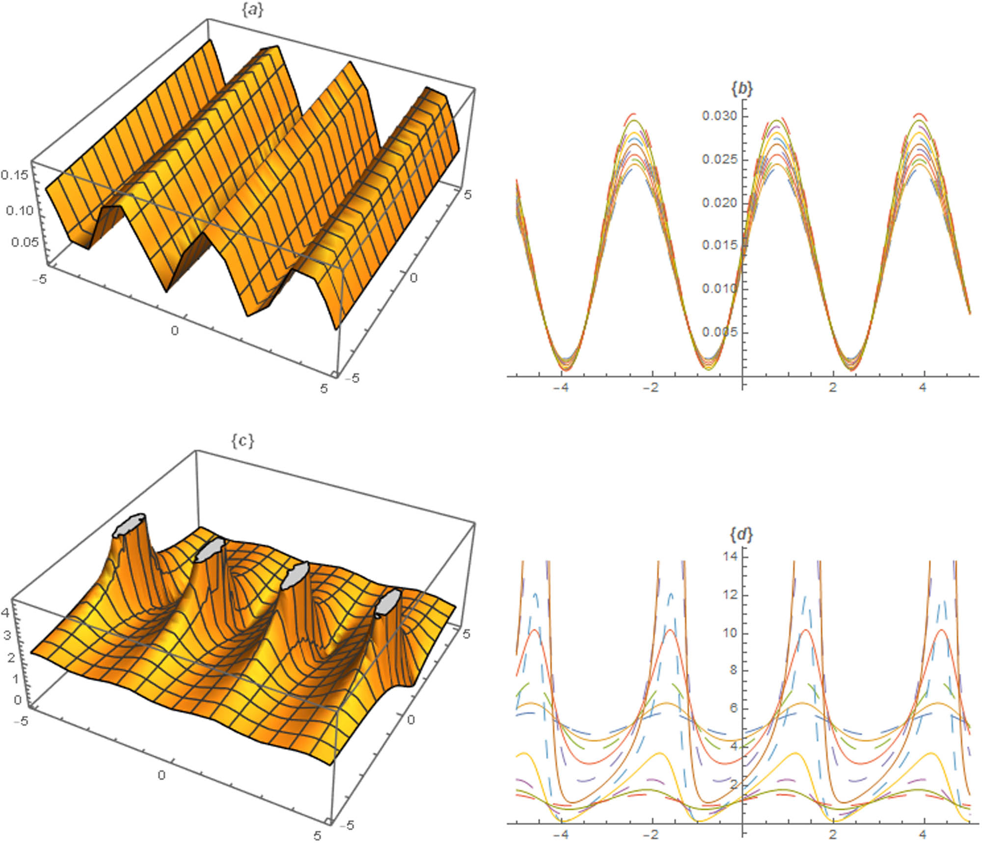
Profiles of solutions
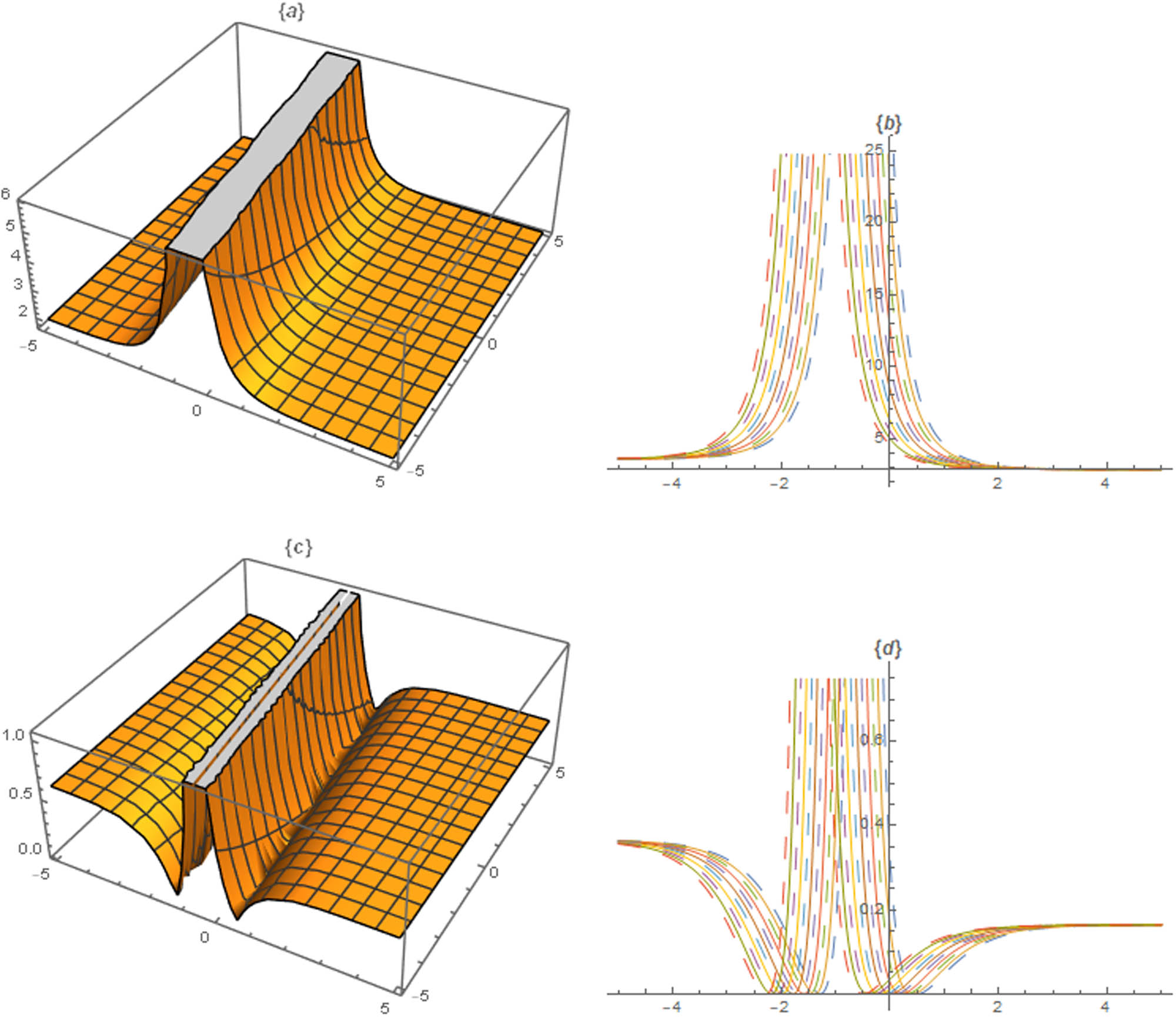
Profile of solutions
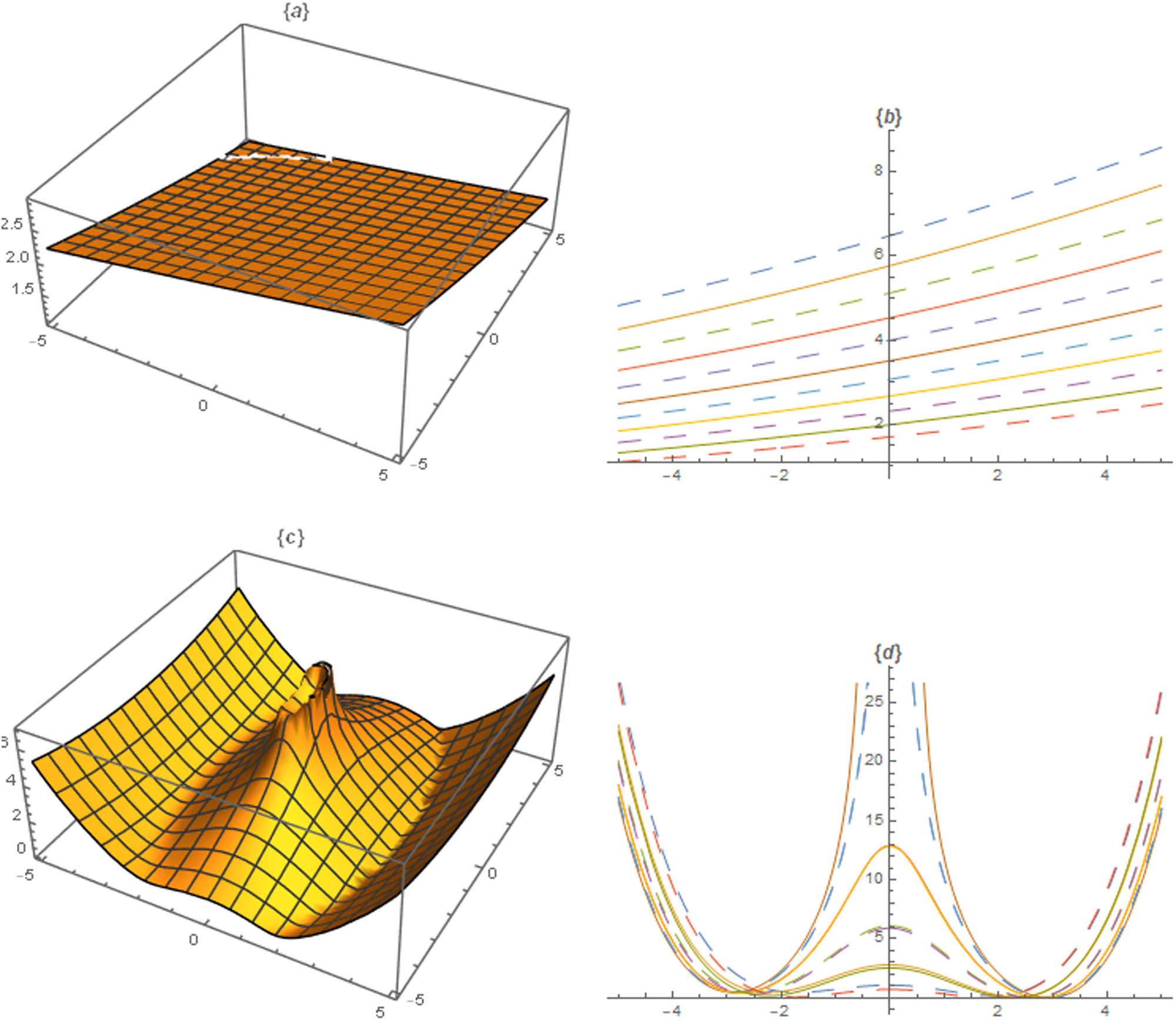
Profiles of solutions

Profiles of solutions
4 Results and discussion
We have discussed our derived results of Eq. (1) via application of three methods with the others results in the literature. Our obtained exact solutions have different forms such as trigonometric function, hyperbolic function, exponential function, and rational function after obtaining the values of
5 Conclusion
In this article, we have constructed several type exact solutions of M-fractional Kairat-II model via successfully implementation of three extended mathematical methods with the support of computational software Mathematica 13.0. The concern model has many applications in optical fibers, which is used to describe the trajectory of optical pulses in optical fibers. The work formally furnishes algorithms for studying newly constructed systems that examine plasma physics, optical communications, oceans and seas, and the differential geometry of curves, among others. The derived exact solutions are in the form of trigonometric function, hyperbolic function, rational function, and exponential function. Moreover, many of the solutions obtained are new and have not been found before. For the physically description, few investigated solutions are plotted 2D and 3D by assigning the particular values to the parameters. This is fact that in current existing literature only two authors [34,35] derived few results of the concern model but here we have established many type exact solutions of Eq. (1). The constructed results show that the applied techniques are trustworthy, competent, and dominant in the analysis of various nonlinear fractional differential equations in diverse field of nonlinear science.
-
Funding information: The authors state no funding involved.
-
Author contributions: A. R. Seadawy: methodology, conceptualization, software, resources and planning, writing original draft. A. Ali: formal analysis, investigation, validation, review, and editing. Ahmet Bekir: supervision, project administration, visualizations, review, and editing. Ali Altalbe: funding acquisition, methodology, investigation, writing original draft. Murat Alp: formal analysis, methodology, validation, review, and editing. All authors have accepted responsibility for the entire content of this manuscript and approved its submission.
-
Conflict of interest: The authors state no conflict of interest.
-
Data availability statement: The datasets used and/or analyzed during the current study available from the corresponding author on reasonable request.
References
[1] Khater MM, Ghanbari B, Nisar KS, Kumar D Novel exact solutions of the fractional Bogoyavlensky-Konopelchenko equation involving the Atangana-Baleanu-Riemann derivative. Alex Eng J. 2020;59(5):2957–67. 10.1016/j.aej.2020.03.032Search in Google Scholar
[2] Ali HM, Ali AS, Mahmoud M, Abdel-Aty AH. Analytical approximate solutions of fractional nonlinear Drinfeld-Sokolov-Wilson model using modified Mittag–Leffer function. J Ocean Eng Sci. 2022. 10.1016/j.joes.2022.06.006Search in Google Scholar
[3] Zafar A, Raheel M, Ali MR, Myrzakulova Z, Bekir A, Myrzakulov R. Exact solutions of M-fractional Kuralay equation via three analytical schemes. Symmetry. 2023;15(10):1862. 10.3390/sym15101862Search in Google Scholar
[4] Yesmakhanova K, Myrzakulova Z, Myrzakulov R, Nugmanova G. Soliton surfaces induced by the Kuralay, Kairat and Akbota equations, July 2023. In: Conference: 15th Symposium on Integrable Systems, Bialystok, Poland, June 29–30. 2023. 10.13140/RG.2.2.16410.41928. Search in Google Scholar
[5] Faridi WA, Bakar MA, Myrzakulova Z, Myrzakulov R, Akgul A, Eldin SM. The formation of solitary wave solutions and their propagation for Kuralay equation. Results Phys. 2023;52(2):2211–3797. 10.1016/j.rinp.2023.106774Search in Google Scholar
[6] Mathanaranjan T. Optical soliton, linear stability analysis and conservation laws via multipliers to the integrable Kuralay equation. Optik. 2023;290:171266. 10.1016/j.ijleo.2023.171266Search in Google Scholar
[7] Kong H-Y, Guo R. Dynamic behaviors of novel nonlinear wave solutions for the Akbota equation. Optik. 2023;282:170863. 10.1016/j.ijleo.2023.170863Search in Google Scholar
[8] Demirbilek U, Ala V, Mamedov KR. Exact solutions of conformable time fractional Zoomeron equation via IBSEFM. Appl Math A J Chin Univ. 2021;36:554–63. 10.1007/s11766-021-4145-3Search in Google Scholar
[9] Hong B, Wang J. Exact solutions for the generalized Atangana-Baleanu-Riemann fractional (3+1)-Dimensional Kadomtsev–Petviashvili equation. Symmetry. 2022;15(1):3. 10.3390/sym15010003Search in Google Scholar
[10] Fadhal E, Akbulut A, Kaplan M, Awadalla M, Abuasbeh K. Extraction of exact solutions of higher order Sasa–Satsuma equation in the sense of beta derivative. Symmetry. 2022;14(11):2390. 10.3390/sym14112390Search in Google Scholar
[11] Sahoo S, Saha R, Santanu, Abdou MAM, Inc M, Chu Y-M. New soliton solutions of fractional Jaulent-Miodek system with symmetry analysis. Symmetry. 2020;12(6):1001. 10.3390/sym12061001Search in Google Scholar
[12] Aniqa A, Ahmad J. Soliton solution of fractional Sharma-Tasso-Olever equation via an effcient (G∕G′)-expansion method. Ain Shams Eng J. 2022;13(1):101528. 10.1016/j.asej.2021.06.014Search in Google Scholar
[13] Riaz MB, Wojciechowski A, Oros GI, Rahman RU. Soliton solutions and sensitive analysis of modified equal-width equation using fractional operators. Symmetry. 2022. 14(8):1731. 10.3390/sym14081731Search in Google Scholar
[14] Faridi WA, Bakar MA, Akgul A, Abd El-Rahman M, El Din SM. Exact fractional soliton solutions of thin-flim ferroelectric material equation by analytical approaches. Alex Eng J. 2023;78:483–97. 10.1016/j.aej.2023.07.049Search in Google Scholar
[15] Roshid MM, Rahman MM, Bashar MH, Hossain MM, Mannaf MA, et al. Dynamical simulation of wave solutions for the M-fractional Lonngren-wave equation using two distinct methods. Alex Eng J. 2023;81:460–8. 10.1016/j.aej.2023.09.045Search in Google Scholar
[16] Alam MN, Aktar S, Tunc C. New solitary wave structures to time fractional biological population model. J Math Anal. 2020;11(3):59–70. Search in Google Scholar
[17] Yu J. Some new exact wave solutions for the ZK-BBM equation. J Appl Sci Eng. 2022;26(7):981–8. Search in Google Scholar
[18] Zafar A, Ali KK, Raheel M, Nisar KS, Bekir A. Abundant M-fractional optical solitons to the pertubed Gerdjikov-Ivanov equation treating the mathematical nonlinear optics. Opt Quantum Electr. 2022;54(1):25. 10.1007/s11082-021-03394-wSearch in Google Scholar
[19] Raheel M, Zafar A, Inc M, Tala-Tebue E. Optical solitons to time-fractional Sasa–Satsuma higher-order non-linear Schrodinger equation via three analytical techniques. Opt Quantum Electr. 2023;55(4):307. 10.1007/s11082-023-04565-7Search in Google Scholar
[20] Chen Z, Manafan J, Raheel M, Zafar A, Alsaikhan F, Abotaleb M. Extracting the exact solitons of time-fractional three coupled nonlinear Maccarias system with complex form via four different methods. Results Phys. 2022;36:105400. 10.1016/j.rinp.2022.105400Search in Google Scholar
[21] Zafa A, Raheel M, Hosseini K, Mirzazadeh M, Salahshour S, Park C, et al. Diverse approaches to search for solitary wave solutions of the fractional modified Camassa-Holm equation. Results Phys. 2021;31:104882. 10.1016/j.rinp.2021.104882Search in Google Scholar
[22] Razzaq W, Habib M, Nadeem M, Zafa A, Khan I, Mwanakatwea PK. Solitary wave solutions of conformable time fractional equations using modified simplest equation method. Complexity. 2022;2022. 10.1155/2022/8705388Search in Google Scholar
[23] Razzaq W, Zafa A, Akbulut A. The modified simplest equation procedure for conformable time-fractional Boussinesq equations. Int J Modern Phys B. 2022;36(17):2250095. 10.1142/S0217979222500953Search in Google Scholar
[24] Barman HK, Roy R, Mahmud F, Akbar MA, Osman MS. Harmonizing wave solutions to the Fokas-Lenells model through the generalized Kudryashov method. Optik. 2021;229:166294. 10.1016/j.ijleo.2021.166294Search in Google Scholar
[25] Ghazanfar S, Ahmed N, Iqbal MS, Akgul A, Bayram M, De la Sen M. Imaging ultrasound propagation using the Westervelt equation by the generalized Kudryashov and modified Kudryashov methods. Appl Sci. 2022;12(22):11813. 10.3390/app122211813Search in Google Scholar
[26] Akter R, Sarker S, Adhikary A, Ali Akbar M, Dey P, MS Osman. Dynamics of geometric shape solutions for space-time fractional modified equal width equation with beta derivative. Partial Differ Equ Appl Math. 2024;11:100841. 10.1016/j.padiff.2024.100841Search in Google Scholar
[27] Haque A, Islam MT, Akbar MA, Osman MS. Analysis of the propagation of nonlinear waves arise in the Heisenberg ferromagnetic spin chain. Opt Quantum Electr. 2024;56:1381. 10.1007/s11082-024-07181-1Search in Google Scholar
[28] Dehingia K, Boulaaras S, Hinçal E, Hosseini K, Abdeljawad T, MS Osman. On the dynamics of a financial system with the effect financial information. Alex Eng J. 2024;106:438–47. 10.1016/j.aej.2024.08.049Search in Google Scholar
[29] Raza N, Osman MS, A.-H. Abdel-Aty, Abdel-Khalek S, Besbes HR. Optical solitons of space-time fractional Fokas-Lenells equation with two versatile integration architectures. Adv Differ Equ. 2020;2020:1–15. 10.1186/s13662-020-02973-7Search in Google Scholar
[30] Y.-Q. Chen, Y.-H. Tang, Manafian J, Rezazadeh H, Osman MS. Dark wave, rogue wave and perturbation solutions of Ivancevic option pricing model. Nonlinear Dyn. 2021;105:2539–48. 10.1007/s11071-021-06642-6Search in Google Scholar
[31] Akinyemi L., Senol M, Osman MS. Analytical and approximate solutions of nonlinear Schrödinger equation with higher dimension in the anomalous dispersion regime. J Ocean Eng Sci. 2022;7:143–54. 10.1016/j.joes.2021.07.006Search in Google Scholar
[32] Iqbal MA, Hamid Ganie A, Miah MM, Osman MS. Extracting the ultimate new soliton solutions of some nonlinear time fractional PDEs via the conformable fractional derivative. Fract Fract. 2024;8(4):210. 10.3390/fractalfract8040210Search in Google Scholar
[33] Özkan YS, Yaşar E, Osman MS. Novel multiple soliton and front wave solutions for the 3D-Vakhnenko-Parkes equation. Modern Phys Lett B. 2022;36(9):2250003. 10.1142/S0217984922500038Search in Google Scholar
[34] Myrzakulova Z, Manukure S, Myrzakulov R, Nugmanova G. Integrability, geometry and wave solutions of some Kairat equations. 2023. arXiv:2307.00027v3. Search in Google Scholar
[35] Awadalla M, Zafar A, Taishiyeva A, Raheel M, Myrzakulov R, Bekir A. Exact soliton solutions of M-fractional Kairat-II and Kairat-X equations via three analytical methods. Preprint. 2023. 10.13140/RG.2.2.18605.26080. Search in Google Scholar
[36] Sulaiman TA, Yel G, Bulut H. M-fractional solitons and periodic wave solutions to the Hirota- Maccari system. Modern Phys Lett B. 2019;33:1950052. 10.1142/S0217984919500520Search in Google Scholar
[37] Vanterler J, Sousa DAC, Capelas E, DE Oliveira. A new truncated M-fractional derivative type unifying some fractional derivative types with classical properties. Int J Anal Appl. 2018;16(1):83–96. Search in Google Scholar
[38] Iqbal M, Lu D, Alammari M, Seadawy AR, Alsubaie NE, Umurzakhova Z, et al. A construction of novel soliton solutions to the nonlinear fractional Kairat-II equation through computational simulation. Opt Quantum Electr. 2024;56(845):845. 10.1007/s11082-024-06467-8Search in Google Scholar
[39] Muhammad J, Rehman SU, Nasreen N, Bilal M, Younas U. Exploring the fractional effect to the optical wave propagation for the extended Kairat-II equation. Nonlinear Dynam. 2025;113(2):1501–12. 10.1007/s11071-024-10139-3Search in Google Scholar
[40] Ali A, Seadawy AR, Lu D. Soliton solutions of the nonlinear Schrödinger equation with the dual power law nonlinearity and resonant nonlinear Schrödinger equation and their modulation instability analysis. Optik. 2017;145:79–88. 10.1016/j.ijleo.2017.07.016Search in Google Scholar
[41] Ali A, Seadawy AR, Lu D. Dispersive solitary wave soliton solutions of (2+1)-dimensional Boussineq dynamical equation via extended simple equation method. J King Saud Univ Sci. 2019;31:653–8. 10.1016/j.jksus.2017.12.015Search in Google Scholar
[42] Seadawy A, Ali A, Aljahdaly N. The nonlinear integro-differential Ito dynamical equation via three modified mathematical methods and its analytical solutions. Open Phys. 2020;18:24–32. 10.1515/phys-2020-0004Search in Google Scholar
[43] Seadawy A, Aliy A, Jhangeer A. Analytical methods: Nonlinear longitudinal wave equation in a magnetoelectro-elastic circular rod, foam drainage and modified Degasperis-Procesi models arising in nonlinear water wave models. Modern Phys Lett B. 2020;34(26):2050278. 10.1142/S0217984920502784Search in Google Scholar
[44] Seadawy AR, Ali A. Novel wave behaviors of the generalized Kadomtsev–Petviashvili modified equal Width-Burgers equation via modified mathematical methods. Int J Modern Phys B. 2023;37(20):2350198. 10.1142/S0217979223501989Search in Google Scholar
[45] Alruwaili AD, Seadawy AR, Ali A, Aldandani MM. Dynamical and physical characteristics of soliton solutions to the (2+1)-dimensional Konopelchenko-Dubrovsky system. Open Phys. 2023;21:20230129. 10.1515/phys-2023-0129Search in Google Scholar
[46] Seadawy AR, Ali A, Altalbe A, Bekir A. Exact solutions of the (3+1)-generalized fractional nonlinear wave equation with gas bubbles. Sci Reports (natureportfolio). 2024;14:1862. 10.1038/s41598-024-52249-3Search in Google Scholar PubMed PubMed Central
[47] Zhu S. The extended (G∕G′)-expansion method and travelling wave solutions of nonlinear evolution equations. Math Comput Appl. 2010;15(5):924–9. 10.3390/mca15050924Search in Google Scholar
[48] E. M. E. Zayed, Al-Joudi S. Applications of an extended (G∕G′)-expansion method to find exact solutions of nonlinear PDEs in mathematical physics. Math Problems Eng. 2010;2010:768573. 10.1155/2010/768573Search in Google Scholar
[49] Chen G, Xin X, Liu H. The improved exp(−Ψ(ξ))-expansion method and new exact solutions of nonlinear evolution equations in mathematical physics. Adv Math Phys. 2019;2019:4354310. 10.1155/2019/4354310Search in Google Scholar
[50] Khater MMA. Extended exp(−Ψ(ξ))-expansion method for solving the generalized Hirota-Satsuma coupled KdV system. Math Decision Sci. 2015;15(7):1–10. Search in Google Scholar
[51] Khan MI, Marwat DN, Sabiu J, Inc M. Exact solutions of Shynaray-IIA equation (S-IIAE) using the improved modified Sardar sub-equation method. Opt Quantum Electr. 2024;56:459. 10.1007/s11082-023-06051-6Search in Google Scholar
[52] Ali K, Seadawy AR, Aziz N, Rizvi STR. Soliton solutions to generalized (2+1)-dimensional Hietarinta-type equation and resonant NLSE along with stability analysis. Int J Modern Phys B. 2024;38:2450009. 10.1142/S0217979224500097Search in Google Scholar
© 2025 the author(s), published by De Gruyter
This work is licensed under the Creative Commons Attribution 4.0 International License.
Articles in the same Issue
- Research Articles
- Single-step fabrication of Ag2S/poly-2-mercaptoaniline nanoribbon photocathodes for green hydrogen generation from artificial and natural red-sea water
- Abundant new interaction solutions and nonlinear dynamics for the (3+1)-dimensional Hirota–Satsuma–Ito-like equation
- A novel gold and SiO2 material based planar 5-element high HPBW end-fire antenna array for 300 GHz applications
- Explicit exact solutions and bifurcation analysis for the mZK equation with truncated M-fractional derivatives utilizing two reliable methods
- Optical and laser damage resistance: Role of periodic cylindrical surfaces
- Numerical study of flow and heat transfer in the air-side metal foam partially filled channels of panel-type radiator under forced convection
- Water-based hybrid nanofluid flow containing CNT nanoparticles over an extending surface with velocity slips, thermal convective, and zero-mass flux conditions
- Dynamical wave structures for some diffusion--reaction equations with quadratic and quartic nonlinearities
- Solving an isotropic grey matter tumour model via a heat transfer equation
- Study on the penetration protection of a fiber-reinforced composite structure with CNTs/GFP clip STF/3DKevlar
- Influence of Hall current and acoustic pressure on nanostructured DPL thermoelastic plates under ramp heating in a double-temperature model
- Applications of the Belousov–Zhabotinsky reaction–diffusion system: Analytical and numerical approaches
- AC electroosmotic flow of Maxwell fluid in a pH-regulated parallel-plate silica nanochannel
- Interpreting optical effects with relativistic transformations adopting one-way synchronization to conserve simultaneity and space–time continuity
- Modeling and analysis of quantum communication channel in airborne platforms with boundary layer effects
- Theoretical and numerical investigation of a memristor system with a piecewise memductance under fractal–fractional derivatives
- Tuning the structure and electro-optical properties of α-Cr2O3 films by heat treatment/La doping for optoelectronic applications
- High-speed multi-spectral explosion temperature measurement using golden-section accelerated Pearson correlation algorithm
- Dynamic behavior and modulation instability of the generalized coupled fractional nonlinear Helmholtz equation with cubic–quintic term
- Study on the duration of laser-induced air plasma flash near thin film surface
- Exploring the dynamics of fractional-order nonlinear dispersive wave system through homotopy technique
- The mechanism of carbon monoxide fluorescence inside a femtosecond laser-induced plasma
- Numerical solution of a nonconstant coefficient advection diffusion equation in an irregular domain and analyses of numerical dispersion and dissipation
- Numerical examination of the chemically reactive MHD flow of hybrid nanofluids over a two-dimensional stretching surface with the Cattaneo–Christov model and slip conditions
- Impacts of sinusoidal heat flux and embraced heated rectangular cavity on natural convection within a square enclosure partially filled with porous medium and Casson-hybrid nanofluid
- Stability analysis of unsteady ternary nanofluid flow past a stretching/shrinking wedge
- Solitonic wave solutions of a Hamiltonian nonlinear atom chain model through the Hirota bilinear transformation method
- Bilinear form and soltion solutions for (3+1)-dimensional negative-order KdV-CBS equation
- Solitary chirp pulses and soliton control for variable coefficients cubic–quintic nonlinear Schrödinger equation in nonuniform management system
- Influence of decaying heat source and temperature-dependent thermal conductivity on photo-hydro-elasto semiconductor media
- Dissipative disorder optimization in the radiative thin film flow of partially ionized non-Newtonian hybrid nanofluid with second-order slip condition
- Bifurcation, chaotic behavior, and traveling wave solutions for the fractional (4+1)-dimensional Davey–Stewartson–Kadomtsev–Petviashvili model
- New investigation on soliton solutions of two nonlinear PDEs in mathematical physics with a dynamical property: Bifurcation analysis
- Mathematical analysis of nanoparticle type and volume fraction on heat transfer efficiency of nanofluids
- Creation of single-wing Lorenz-like attractors via a ten-ninths-degree term
- Optical soliton solutions, bifurcation analysis, chaotic behaviors of nonlinear Schrödinger equation and modulation instability in optical fiber
- Chaotic dynamics and some solutions for the (n + 1)-dimensional modified Zakharov–Kuznetsov equation in plasma physics
- Fractal formation and chaotic soliton phenomena in nonlinear conformable Heisenberg ferromagnetic spin chain equation
- Single-step fabrication of Mn(iv) oxide-Mn(ii) sulfide/poly-2-mercaptoaniline porous network nanocomposite for pseudo-supercapacitors and charge storage
- Novel constructed dynamical analytical solutions and conserved quantities of the new (2+1)-dimensional KdV model describing acoustic wave propagation
- Tavis–Cummings model in the presence of a deformed field and time-dependent coupling
- Spinning dynamics of stress-dependent viscosity of generalized Cross-nonlinear materials affected by gravitationally swirling disk
- Design and prediction of high optical density photovoltaic polymers using machine learning-DFT studies
- Robust control and preservation of quantum steering, nonlocality, and coherence in open atomic systems
- Coating thickness and process efficiency of reverse roll coating using a magnetized hybrid nanomaterial flow
- Dynamic analysis, circuit realization, and its synchronization of a new chaotic hyperjerk system
- Decoherence of steerability and coherence dynamics induced by nonlinear qubit–cavity interactions
- Finite element analysis of turbulent thermal enhancement in grooved channels with flat- and plus-shaped fins
- Modulational instability and associated ion-acoustic modulated envelope solitons in a quantum plasma having ion beams
- Statistical inference of constant-stress partially accelerated life tests under type II generalized hybrid censored data from Burr III distribution
- On solutions of the Dirac equation for 1D hydrogenic atoms or ions
- Entropy optimization for chemically reactive magnetized unsteady thin film hybrid nanofluid flow on inclined surface subject to nonlinear mixed convection and variable temperature
- Stability analysis, circuit simulation, and color image encryption of a novel four-dimensional hyperchaotic model with hidden and self-excited attractors
- A high-accuracy exponential time integration scheme for the Darcy–Forchheimer Williamson fluid flow with temperature-dependent conductivity
- Novel analysis of fractional regularized long-wave equation in plasma dynamics
- Development of a photoelectrode based on a bismuth(iii) oxyiodide/intercalated iodide-poly(1H-pyrrole) rough spherical nanocomposite for green hydrogen generation
- Investigation of solar radiation effects on the energy performance of the (Al2O3–CuO–Cu)/H2O ternary nanofluidic system through a convectively heated cylinder
- Quantum resources for a system of two atoms interacting with a deformed field in the presence of intensity-dependent coupling
- Studying bifurcations and chaotic dynamics in the generalized hyperelastic-rod wave equation through Hamiltonian mechanics
- A new numerical technique for the solution of time-fractional nonlinear Klein–Gordon equation involving Atangana–Baleanu derivative using cubic B-spline functions
- Interaction solutions of high-order breathers and lumps for a (3+1)-dimensional conformable fractional potential-YTSF-like model
- Hydraulic fracturing radioactive source tracing technology based on hydraulic fracturing tracing mechanics model
- Numerical solution and stability analysis of non-Newtonian hybrid nanofluid flow subject to exponential heat source/sink over a Riga sheet
- Numerical investigation of mixed convection and viscous dissipation in couple stress nanofluid flow: A merged Adomian decomposition method and Mohand transform
- Effectual quintic B-spline functions for solving the time fractional coupled Boussinesq–Burgers equation arising in shallow water waves
- Analysis of MHD hybrid nanofluid flow over cone and wedge with exponential and thermal heat source and activation energy
- Solitons and travelling waves structure for M-fractional Kairat-II equation using three explicit methods
- Impact of nanoparticle shapes on the heat transfer properties of Cu and CuO nanofluids flowing over a stretching surface with slip effects: A computational study
- Computational simulation of heat transfer and nanofluid flow for two-sided lid-driven square cavity under the influence of magnetic field
- Irreversibility analysis of a bioconvective two-phase nanofluid in a Maxwell (non-Newtonian) flow induced by a rotating disk with thermal radiation
- Hydrodynamic and sensitivity analysis of a polymeric calendering process for non-Newtonian fluids with temperature-dependent viscosity
- Exploring the peakon solitons molecules and solitary wave structure to the nonlinear damped Kortewege–de Vries equation through efficient technique
- Modeling and heat transfer analysis of magnetized hybrid micropolar blood-based nanofluid flow in Darcy–Forchheimer porous stenosis narrow arteries
- Activation energy and cross-diffusion effects on 3D rotating nanofluid flow in a Darcy–Forchheimer porous medium with radiation and convective heating
- Insights into chemical reactions occurring in generalized nanomaterials due to spinning surface with melting constraints
- Influence of a magnetic field on double-porosity photo-thermoelastic materials under Lord–Shulman theory
- Soliton-like solutions for a nonlinear doubly dispersive equation in an elastic Murnaghan's rod via Hirota's bilinear method
- Analytical and numerical investigation of exact wave patterns and chaotic dynamics in the extended improved Boussinesq equation
- Nonclassical correlation dynamics of Heisenberg XYZ states with (x, y)-spin--orbit interaction, x-magnetic field, and intrinsic decoherence effects
- Exact traveling wave and soliton solutions for chemotaxis model and (3+1)-dimensional Boiti–Leon–Manna–Pempinelli equation
- Unveiling the transformative role of samarium in ZnO: Exploring structural and optical modifications for advanced functional applications
- On the derivation of solitary wave solutions for the time-fractional Rosenau equation through two analytical techniques
- Analyzing the role of length and radius of MWCNTs in a nanofluid flow influenced by variable thermal conductivity and viscosity considering Marangoni convection
- Advanced mathematical analysis of heat and mass transfer in oscillatory micropolar bio-nanofluid flows via peristaltic waves and electroosmotic effects
- Exact bound state solutions of the radial Schrödinger equation for the Coulomb potential by conformable Nikiforov–Uvarov approach
- Some anisotropic and perfect fluid plane symmetric solutions of Einstein's field equations using killing symmetries
- Nonlinear dynamics of the dissipative ion-acoustic solitary waves in anisotropic rotating magnetoplasmas
- Curves in multiplicative equiaffine plane
- Exact solution of the three-dimensional (3D) Z2 lattice gauge theory
- Propagation properties of Airyprime pulses in relaxing nonlinear media
- Symbolic computation: Analytical solutions and dynamics of a shallow water wave equation in coastal engineering
- Wave propagation in nonlocal piezo-photo-hygrothermoelastic semiconductors subjected to heat and moisture flux
- Comparative reaction dynamics in rotating nanofluid systems: Quartic and cubic kinetics under MHD influence
- Laplace transform technique and probabilistic analysis-based hypothesis testing in medical and engineering applications
- Physical properties of ternary chloro-perovskites KTCl3 (T = Ge, Al) for optoelectronic applications
- Gravitational length stretching: Curvature-induced modulation of quantum probability densities
- The search for the cosmological cold dark matter axion – A new refined narrow mass window and detection scheme
- A comparative study of quantum resources in bipartite Lipkin–Meshkov–Glick model under DM interaction and Zeeman splitting
- PbO-doped K2O–BaO–Al2O3–B2O3–TeO2-glasses: Mechanical and shielding efficacy
- Nanospherical arsenic(iii) oxoiodide/iodide-intercalated poly(N-methylpyrrole) composite synthesis for broad-spectrum optical detection
- Sine power Burr X distribution with estimation and applications in physics and other fields
- Numerical modeling of enhanced reactive oxygen plasma in pulsed laser deposition of metal oxide thin films
- Dynamical analyses and dispersive soliton solutions to the nonlinear fractional model in stratified fluids
- Computation of exact analytical soliton solutions and their dynamics in advanced optical system
- An innovative approximation concerning the diffusion and electrical conductivity tensor at critical altitudes within the F-region of ionospheric plasma at low latitudes
- An analytical investigation to the (3+1)-dimensional Yu–Toda–Sassa–Fukuyama equation with dynamical analysis: Bifurcation
- Swirling-annular-flow-induced instability of a micro shell considering Knudsen number and viscosity effects
- Numerical analysis of non-similar convection flows of a two-phase nanofluid past a semi-infinite vertical plate with thermal radiation
- MgO NPs reinforced PCL/PVC nanocomposite films with enhanced UV shielding and thermal stability for packaging applications
- Optimal conditions for indoor air purification using non-thermal Corona discharge electrostatic precipitator
- Investigation of thermal conductivity and Raman spectra for HfAlB, TaAlB, and WAlB based on first-principles calculations
- Tunable double plasmon-induced transparency based on monolayer patterned graphene metamaterial
- DSC: depth data quality optimization framework for RGBD camouflaged object detection
- A new family of Poisson-exponential distributions with applications to cancer data and glass fiber reliability
- Numerical investigation of couple stress under slip conditions via modified Adomian decomposition method
- Monitoring plateau lake area changes in Yunnan province, southwestern China using medium-resolution remote sensing imagery: applicability of water indices and environmental dependencies
- Heterodyne interferometric fiber-optic gyroscope
- Exact solutions of Einstein’s field equations via homothetic symmetries of non-static plane symmetric spacetime
- A widespread study of discrete entropic model and its distribution along with fluctuations of energy
- Empirical model integration for accurate charge carrier mobility simulation in silicon MOSFETs
- The influence of scattering correction effect based on optical path distribution on CO2 retrieval
- Anisotropic dissociation and spectral response of 1-Bromo-4-chlorobenzene under static directional electric fields
- Role of tungsten oxide (WO3) on thermal and optical properties of smart polymer composites
- Analysis of iterative deblurring: no explicit noise
- Review Article
- Examination of the gamma radiation shielding properties of different clay and sand materials in the Adrar region
- Erratum
- Erratum to “On Soliton structures in optical fiber communications with Kundu–Mukherjee–Naskar model (Open Physics 2021;19:679–682)”
- Special Issue on Fundamental Physics from Atoms to Cosmos - Part II
- Possible explanation for the neutron lifetime puzzle
- Special Issue on Nanomaterial utilization and structural optimization - Part III
- Numerical investigation on fluid-thermal-electric performance of a thermoelectric-integrated helically coiled tube heat exchanger for coal mine air cooling
- Special Issue on Nonlinear Dynamics and Chaos in Physical Systems
- Analysis of the fractional relativistic isothermal gas sphere with application to neutron stars
- Abundant wave symmetries in the (3+1)-dimensional Chafee–Infante equation through the Hirota bilinear transformation technique
- Successive midpoint method for fractional differential equations with nonlocal kernels: Error analysis, stability, and applications
- Novel exact solitons to the fractional modified mixed-Korteweg--de Vries model with a stability analysis