Solitary chirp pulses and soliton control for variable coefficients cubic–quintic nonlinear Schrödinger equation in nonuniform management system
-
Rehab M. El-Shiekh
 and
Mahmoud Gaballah
and
Mahmoud Gaballah

Abstract
This study investigates the variable coefficient cubic–quintic nonlinear Schrödinger equation, which models the propagation of ultrashort femtosecond pulses in optical fibers and three-body recombination losses in Bose–Einstein condensates. Using a mapping technique combined with an extended chirp wave transformation, 20 chirp wave solutions were derived, including bright and dark solitons, kink waves, periodic and singular waves. These solutions encompass previously reported results and introduce novel ones. Three-dimensional plots illustrate the soliton and kink chirp wave solutions for both constant and exponentially varying group velocity dispersion (GVD) and Raman effect parameters. Analysis reveals that the sign of the Raman effect parameter influences the soliton type, yielding bright solitons for positive values and dark solitons for negative values. Furthermore, both GVD and Raman effect significantly impact the wave shape, inducing oscillations in the case of exponentially distributed fiber. The stability of the soliton wave solution is also analyzed. These diverse wave profiles have potential applications in nonlinear optics and plasma physics.
1 Introduction
The variable coefficient nonlinear Schrödinger (VCNLS) equation is a generalization of the nonlinear Schrödinger (NLS) equation that allows for the coefficients to vary with position and time. This makes it a more versatile equation for modeling a wider range of physical phenomena. It can be used to describe the propagation of light pulses through optical fibers and other nonlinear materials with varying properties [1], the behavior of ultracold atoms trapped in inhomogeneous potentials [2], the dynamics of plasma waves in nonuniform plasmas [3], and the propagation of sound waves through nonlinear materials with variable properties [4]. This equation, which generalizes the NLS equation by allowing for variable coefficients, is essential for studying the complex interactions between waves and their environments [4–10]. The VCNLS equation can be written as:
where
One of the very important VCNLS equations is the variable coefficients cubic–quintic nonlinear Schrödinger (VCQNLS) equation, which can be used to describe the ultrashort optical pulses obtained by increasing the intensity of the incident light field in the presence of higher-order nonlinear terms, like self-steepening and self-frequency shift [11,12]. Additionally, the existence of quintic nonlinearity is vital for studying three-body recombination losses in the circumstances of Bose–Einstein condensates [12–17]. Therefore, in this work, we are going to study the VCQNLS, which is given by
By comparison between Eqs (1) and (2), we can see that there are two additional terms, the quintic term
The VCQNLS Eq. (2) was investigated by Wang et al. [11] using a similarity transformation. They converted it into the KE equation with constant coefficients and employed known solutions from the literature to derive one and two soliton solutions under specific conditions on the variable coefficients. Subsequently, Xie and Yan [12] utilized the bilinear form to construct one and two soliton solutions, albeit under different relationships between the variable coefficients.
However, the mentioned research works focus on soliton wave-type solutions, and to the best of our knowledge, other wave solutions like kink and periodic types have not been obtained before. From our review on constant coefficients version of Eq. (2) [12–24], we have found that chirp wave solution was obtained, and this inspired us to generalize the chirp wave transformation to be dependent on variable functions and combined it with the mapping method [26–28] to be able to find different chirp wave solutions for Eq. (2). Moreover, it was the first time the mapping method was applied to nonlinear partial differential equations (NPDEs) with variable coefficients like the VCQNLS equation.
This study is devoted to five sections, Section 1 gives the introduction and literature review, Section 2 describes methodology, in Section 3, the application of the methodology and novel wave solutions are given, then in Section 4, physical applications containing dynamic behavior of some chirp wave solutions and its stability are given, and, finally, conclusion and important remarks are given in Section 5.
2 Methodology
In recent times, numerous novel techniques have been explored for solving NPDEs [29–31], then mean focusing has been done on extending and generalizing these methodologies to address NPDEs with variable coefficients [27–31]. One of those techniques is the mapping method introduced by Zayed et al. [26–28], it stands out as one such technique with extensive applications in NPDEs featuring constant coefficients. However, its generalization to solve NPDEs with variable coefficients is yet to be realized. Based on our literature review of the constant KE equation [21–25], we have devised a generalization of the traveling wave transformation presented therein. This generalization enables us to derive chirp solitary wave for the VCQNLS, as follows:
(1) If a complex NPDE defined as
where
where
(2) By using transformation (4) in Eq. (3), it transformed to an NODE in
(3) If
where
The positive real number
3 Novel solitary waves for the VCQNLS
To derive solitary and periodic chirp wave solutions, we must employ the transformation defined by Eq. (4) to convert the VCQNLS into an NODE. Subsequently, we separate the NODE into its real and imaginary components as follows:
By integrating Eq. (9) for
Substituting Eq. (10) in Eq. (8) yields the following NODE:
Divide all terms of Eq. (11) by
Then, assume that the variable coefficients are nonzero constants
We can see that all variable parameters depend on only two variables
From Eq. (6), we should first determine the value of
where
The coeff. of
The coeff. of
The coeff. of
The coeff. of
The coeff. of
The coeff. of
Upon solving the preceding system, we arrive at the following values:
Using the 20 values of
where
4 Physical applications
Chirp waves, whose frequency changes over time, and solitons, self-reinforcing solitary waves, have a complex interplay. Chirp waves can compress solitons, generate new ones, and influence their dynamics [32]. This interaction is crucial in various fields, including optical communications, nonlinear optics, and plasma physics. By understanding and controlling chirp wave-soliton interactions, researchers can advance technologies such as high-speed data transmission, laser systems, and plasma-based energy generation [33–35]. We calculate the chirp for our problem using the following equation:
From Eq. (10),
Using
4.1 Dynamic behavior of solutions
Nonuniform management system refers to a system where the control parameters are not uniform, leading to a more complex and realistic scenario. Therefore, this variability in the VCQNLE coefficients allows it to effectively model the dynamics of nonuniform management systems [11]. By mapping the parameters of the management system to the VCQNLE, we can use the equation to present more complicated phenomena in optics and plasma physics [3–5]. According to that, we will now concentrate on how specific parameters influence wave propagation, drawing primarily from Eqs (39) and (13). Of these, only two parameters significantly impact wave propagation: the group velocity
Case I: To isolate the effects of


In Figure 1(a) and (b), it is clear that in the case of nonlinearity management system where the GVD is taken as a constant value
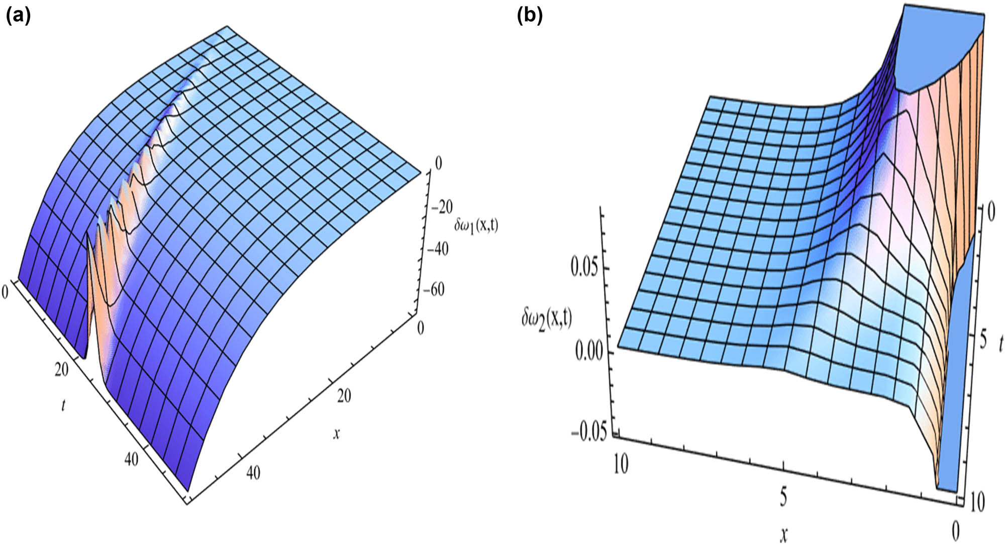
The evolution 3D plot of the bright soliton chirp wave

The 3D plot of the dark soliton chirp wave
4.2 Solution stability
The motion of conservative systems in classical mechanics is described by the Hamiltonian system. The momentum is given as [10]
where
If we take
Therefore, the important conditions for the solitary wave solution
5 Conclusion
Using mapping method combined with variable chirp wave transformation (4), we have successfully constructed different types of chirp wave solutions including bright soliton, dark soliton solutions, kink shaped profiles, and singular periodic solutions of the VCQNLE. We have provided graphical and physical explanations by creating 3D diagrams, illustrating how the variables GVD
The utilization of these obtained solutions shows simplicity, effectiveness, and power of the mapping method.
The visualization of the soliton and kink chirp waves shows that their shape can be changed by controlling the GVD
When we have fixed the value of
The stability of the obtained solutions was studied for
The obtained solutions can have many applications in optic fiber communications and plasma physics.
Acknowledgments
The authors would like to thank the Deanship of Scientific Research, Majmaah University, Saudi Arabia, for funding this work under project Number R-2025-1688.
-
Funding information: This work was funded by the Deanship of Scientific Research, Majmaah University, Saudi Arabia under project Number R-2025-1688.
-
Author contributions: All authors have accepted responsibility for the entire content of this manuscript and approved its submission.
-
Conflict of interest: The authors state no conflict of interest.
-
Data availability statement: All data generated or analysed during this study are included in this published article.
References
[1] Raza N, Hassan Z, Seadawy A. Computational soliton solutions for the variable coefficient nonlinear Schrödinger equation by collective variable method. Opt Quantum Electron. 2021;53:1–16. 10.1007/S11082-021-03052-1/FIGURES/2. Search in Google Scholar
[2] Nchejane JN, Gbenro SO. Nonlinear Schrödinger equations with variable coefficients: numerical integration. J Adv Math Comput Sci. 2022;37:56–69. 10.9734/JAMCS/2022/v37i330442. Search in Google Scholar
[3] Chen SS, Tian B, Qu QX, Li H, Sun Y, Du XX. Alfvén solitons and generalized Darboux transformation for a variable-coefficient derivative nonlinear Schrödinger equation in an inhomogeneous plasma. Chaos Solitons Fractals. 2021;148:111029. 10.1016/J.CHAOS.2021.111029. Search in Google Scholar
[4] González-Gaxiola O, Biswas A, Alzahrani AK, Belic MR. Highly dispersive optical solitons with a polynomial law of refractive index by Laplace-Adomian decomposition. J Comput Electron. 2021;20:1216–23. 10.1007/S10825-021-01710-X/FIGURES/6. Search in Google Scholar
[5] Xu SL, Petrović N, Belić MR, Deng W. Exact solutions for the quintic nonlinear Schrödinger equation with time and space. Nonlinear Dyn. 2016;84:251–9. 10.1007/S11071-015-2426-1/FIGURES/8. Search in Google Scholar
[6] Dai C, Wang Y, Yan C. Chirped and chirp-free self-similar cnoidal and solitary wave solutions of the cubic-quintic nonlinear Schrödinger equation with distributed coefficients. Opt Commun. 2010;283:1489–94. 10.1016/J.OPTCOM.2009.11.082. Search in Google Scholar
[7] El-Shiekh RM, Gaballah M. Novel solitary and periodic waves for the extended cubic (3+1)-dimensional Schrödinger equation. Opt Quantum Electron 2023;55:1–12. 10.1007/S11082-023-04965-9/METRICS. Search in Google Scholar
[8] El-Shiekh RM, Gaballah M. Solitary wave solutions for the variable-coefficient coupled nonlinear Schrödinger equations and Davey-Stewartson system using modified sine-Gordon equation method. J Ocean Eng Sci. 2020;5:180–5. 10.1016/J.JOES.2019.10.003. Search in Google Scholar
[9] El-Shiekh RM, Gaballah M. New rogon waves for the nonautonomous variable coefficients Schrödinger equation. Opt Quantum Electron. 2021;53:1–12. 10.1007/S11082-021-03066-9/FIGURES/3. Search in Google Scholar
[10] Gaballah M, El-Shiekh RM. Novel picosecond wave solutions and soliton control for a higher-order nonlinear Schrödinger equation with variable coefficient. Alexandria Eng. J 2025;114:419–25. 10.1016/J.AEJ.2024.11.078. Search in Google Scholar
[11] Wang P, Feng L, Shang T, Guo L, Cheng G, Du Y. Analytical soliton solutions for the cubic-quintic nonlinear Schrödinger equation with Raman effect in the nonuniform management systems. Nonlinear Dyn. 2015;79:387–95. 10.1007/S11071-014-1672-Y/FIGURES/9. Search in Google Scholar
[12] Xie XY, Yan ZH. Soliton collisions for the Kundu-Eckhaus equation with variable coefficients in an optical fiber. Appl Math Lett. 2018;80:48–53. 10.1016/J.AML.2018.01.003. Search in Google Scholar
[13] Baylndlr C. Rogue wave spectra of the Kundu-Eckhaus equation. Phys Rev E. 2016;93:062215. 10.1103/PHYSREVE.93.062215/FIGURES/9/MEDIUM. Search in Google Scholar
[14] Mirzazadeh M, Yıldırım Y, Yaşar E, Triki H, Zhou Q, Moshokoa SP, et al. Optical solitons and conservation law of Kundu-Eckhaus equation. Optik (Stuttg). 2018;154:551–7. 10.1016/J.IJLEO.2017.10.084. Search in Google Scholar
[15] Kumar D, Manafian J, Hawlader F, Ranjbaran A. New closed form soliton and other solutions of the Kundu-Eckhaus equation via the extended sinh-Gordon equation expansion method. Optik (Stuttg) 2018;160:159–67. 10.1016/J.IJLEO.2018.01.137. Search in Google Scholar
[16] El-Borai MM, El-Owaidy HM, Ahmed HM, Arnous AH, Moshokoa S, Biswas A, et al. Topological and singular soliton solution to Kundu-Eckhaus equation with extended Kudryashov’s method. Optik (Stuttg). 2017;128:57–62. 10.1016/J.IJLEO.2016.10.011. Search in Google Scholar
[17] Rezazadeh H, Korkmaz A, Eslami M, Mirhosseini-Alizamini SM. A large family of optical solutions to Kundu-Eckhaus model by a new auxiliary equation method. Opt Quantum Electron. 2019;51:1–12. 10.1007/S11082-019-1801-4/METRICS. Search in Google Scholar
[18] Xie XY, Tian B, Sun WR, Sun Y. Rogue-wave solutions for the Kundu-Eckhaus equation with variable coefficients in an optical fiber. Nonlinear Dyn. 2015;81:1349–54. 10.1007/S11071-015-2073-6/FIGURES/2. Search in Google Scholar
[19] Wang DS, Guo B, Wang X. Long-time asymptotics of the focusing Kundu-Eckhaus equation with nonzero boundary conditions. J Differ Equ. 2019;266:5209–53. 10.1016/J.JDE.2018.10.053. Search in Google Scholar
[20] Wang X, Yang B, Chen Y, Yang Y. Higher-order rogue wave solutions of the Kundu-Eckhaus equation. Phys Scr. 2014;89:095210. 10.1088/0031-8949/89/9/095210. Search in Google Scholar
[21] Baskonus HM, Bulut H. On the complex structures of Kundu-Eckhaus equation via improved Bernoulli sub-equation function method. Waves Random Complex Media. 2015;25:720–8. 10.1080/17455030.2015.1080392. Search in Google Scholar
[22] Islam SMR, Ahmad H, Khan K, Wang H, Akbar MA, Awwad FA, et al. Stability analysis, phase plane analysis, and isolated soliton solution to the LGH equation in mathematical physics. Open Phys. 2023;21:20230104. 10.1515/PHYS-2023-0104/ASSET/GRAPHIC/J_PHYS-2023-0104_FIG._008.JPG. Search in Google Scholar
[23] El-Shiekh RM, Gaballah M. Ultrashort chirp pulses for Kundu-Eckhaus equation in nonlinear optics. Opt Quantum Electron. 2024;56:1–10. 10.1007/S11082-024-07222-9/METRICS. Search in Google Scholar
[24] Triki H, Sun Y, Biswas A, Zhou Q, Yıldırım Y, Zhong Y, et al. On the existence of chirped algebraic solitary waves in optical fibers governed by Kundu-Eckhaus equation. Results Phys. 2022;34:105272. 10.1016/J.RINP.2022.105272. Search in Google Scholar
[25] Daoui AK, Messouber A, Triki H, Zhou Q, Biswas A, Liu W, et al. Propagation of chirped periodic and localized waves with higher-order effects through optical fibers. Chaos Solitons Fractals. 2021;146:110873. 10.1016/J.CHAOS.2021.110873. Search in Google Scholar
[26] Zayed EME, Alurrfi KAE. Solitons and other solutions for two nonlinear Schrödinger equations using the new mapping method. Optik (Stuttg). 2017;144:132–48. 10.1016/J.IJLEO.2017.06.101. Search in Google Scholar
[27] Zayed EME, Alurrfi KAE, Alshbear RA. On application of the new mapping method to magneto-optic waveguides having Kudryashov’s law of refractive index. Optik (Stuttg). 2023;287:171072. 10.1016/J.IJLEO.2023.171072. Search in Google Scholar
[28] Zayed EME, Alngar MEM, Shohib RMA, Biswas A, Yıldırım Y, Alshomrani AS, et al. Optical solitons having Kudryashov’s self-phase modulation with multiplicative white noise via Itô Calculus using new mapping approach. Optik (Stuttg). 2022;264:169369. 10.1016/J.IJLEO.2022.169369. Search in Google Scholar
[29] Islam SMR, Arafat SMY, Alotaibi H, Inc M. Some optical soliton solution with bifurcation analysis of the paraxial nonlinear Schrödinger equation. Opt Quantum Electron. 2024;56:1–16. 10.1007/S11082-023-05783-9/METRICS. Search in Google Scholar
[30] Islam SMR, Basak US. On traveling wave solutions with bifurcation analysis for the nonlinear potential Kadomtsev-Petviashvili and Calogero-Degasperis equations. Partial Differ Equations Appl Math. 2023;8:100561. 10.1016/J.PADIFF.2023.100561. Search in Google Scholar
[31] Islam SMR, Khan K, Akbar MA. Optical soliton solutions, bifurcation, and stability analysis of the Chen-Lee-Liu model. Results Phys. 2023;51:106620. 10.1016/J.RINP.2023.106620. Search in Google Scholar
[32] Spiess C, Yang Q, Dong X, Renninger WH, Bucklew VG. Chirped dissipative solitons in driven optical resonators. Opt 2021;8(6):861– 9. 10.1364/OPTICA.419771. Search in Google Scholar
[33] Kivshar Y, Agrawal G. Optical solitons: from fibers to photonic crystals. New York: Academic Press; 2003. 10.1016/B978-012410590-4/50012-7Search in Google Scholar
[34] Mandeng LM, Tchawoua C, Tagwo H, Zghal M, Cherif I, Mohamadou A. Role of the input profile asymmetry and the Chirp on the propagation in highly dispersive and nonlinear fibers. J Light Technol 2016;34:5635–41. 10.1109/JLT.2016.2624699. Search in Google Scholar
[35] Cai W, Yang Z, Wu H, Wang L, Zhang J, Zhang L, et al. Effect of chirp on pulse reflection and refraction at a moving temporal boundary. Opt Express. 2022;30:34875–86. 10.1364/OE.462333. Search in Google Scholar PubMed
© 2025 the author(s), published by De Gruyter
This work is licensed under the Creative Commons Attribution 4.0 International License.
Articles in the same Issue
- Research Articles
- Single-step fabrication of Ag2S/poly-2-mercaptoaniline nanoribbon photocathodes for green hydrogen generation from artificial and natural red-sea water
- Abundant new interaction solutions and nonlinear dynamics for the (3+1)-dimensional Hirota–Satsuma–Ito-like equation
- A novel gold and SiO2 material based planar 5-element high HPBW end-fire antenna array for 300 GHz applications
- Explicit exact solutions and bifurcation analysis for the mZK equation with truncated M-fractional derivatives utilizing two reliable methods
- Optical and laser damage resistance: Role of periodic cylindrical surfaces
- Numerical study of flow and heat transfer in the air-side metal foam partially filled channels of panel-type radiator under forced convection
- Water-based hybrid nanofluid flow containing CNT nanoparticles over an extending surface with velocity slips, thermal convective, and zero-mass flux conditions
- Dynamical wave structures for some diffusion--reaction equations with quadratic and quartic nonlinearities
- Solving an isotropic grey matter tumour model via a heat transfer equation
- Study on the penetration protection of a fiber-reinforced composite structure with CNTs/GFP clip STF/3DKevlar
- Influence of Hall current and acoustic pressure on nanostructured DPL thermoelastic plates under ramp heating in a double-temperature model
- Applications of the Belousov–Zhabotinsky reaction–diffusion system: Analytical and numerical approaches
- AC electroosmotic flow of Maxwell fluid in a pH-regulated parallel-plate silica nanochannel
- Interpreting optical effects with relativistic transformations adopting one-way synchronization to conserve simultaneity and space–time continuity
- Modeling and analysis of quantum communication channel in airborne platforms with boundary layer effects
- Theoretical and numerical investigation of a memristor system with a piecewise memductance under fractal–fractional derivatives
- Tuning the structure and electro-optical properties of α-Cr2O3 films by heat treatment/La doping for optoelectronic applications
- High-speed multi-spectral explosion temperature measurement using golden-section accelerated Pearson correlation algorithm
- Dynamic behavior and modulation instability of the generalized coupled fractional nonlinear Helmholtz equation with cubic–quintic term
- Study on the duration of laser-induced air plasma flash near thin film surface
- Exploring the dynamics of fractional-order nonlinear dispersive wave system through homotopy technique
- The mechanism of carbon monoxide fluorescence inside a femtosecond laser-induced plasma
- Numerical solution of a nonconstant coefficient advection diffusion equation in an irregular domain and analyses of numerical dispersion and dissipation
- Numerical examination of the chemically reactive MHD flow of hybrid nanofluids over a two-dimensional stretching surface with the Cattaneo–Christov model and slip conditions
- Impacts of sinusoidal heat flux and embraced heated rectangular cavity on natural convection within a square enclosure partially filled with porous medium and Casson-hybrid nanofluid
- Stability analysis of unsteady ternary nanofluid flow past a stretching/shrinking wedge
- Solitonic wave solutions of a Hamiltonian nonlinear atom chain model through the Hirota bilinear transformation method
- Bilinear form and soltion solutions for (3+1)-dimensional negative-order KdV-CBS equation
- Solitary chirp pulses and soliton control for variable coefficients cubic–quintic nonlinear Schrödinger equation in nonuniform management system
- Influence of decaying heat source and temperature-dependent thermal conductivity on photo-hydro-elasto semiconductor media
- Dissipative disorder optimization in the radiative thin film flow of partially ionized non-Newtonian hybrid nanofluid with second-order slip condition
- Bifurcation, chaotic behavior, and traveling wave solutions for the fractional (4+1)-dimensional Davey–Stewartson–Kadomtsev–Petviashvili model
- New investigation on soliton solutions of two nonlinear PDEs in mathematical physics with a dynamical property: Bifurcation analysis
- Mathematical analysis of nanoparticle type and volume fraction on heat transfer efficiency of nanofluids
- Creation of single-wing Lorenz-like attractors via a ten-ninths-degree term
- Optical soliton solutions, bifurcation analysis, chaotic behaviors of nonlinear Schrödinger equation and modulation instability in optical fiber
- Chaotic dynamics and some solutions for the (n + 1)-dimensional modified Zakharov–Kuznetsov equation in plasma physics
- Fractal formation and chaotic soliton phenomena in nonlinear conformable Heisenberg ferromagnetic spin chain equation
- Single-step fabrication of Mn(iv) oxide-Mn(ii) sulfide/poly-2-mercaptoaniline porous network nanocomposite for pseudo-supercapacitors and charge storage
- Novel constructed dynamical analytical solutions and conserved quantities of the new (2+1)-dimensional KdV model describing acoustic wave propagation
- Tavis–Cummings model in the presence of a deformed field and time-dependent coupling
- Spinning dynamics of stress-dependent viscosity of generalized Cross-nonlinear materials affected by gravitationally swirling disk
- Design and prediction of high optical density photovoltaic polymers using machine learning-DFT studies
- Robust control and preservation of quantum steering, nonlocality, and coherence in open atomic systems
- Coating thickness and process efficiency of reverse roll coating using a magnetized hybrid nanomaterial flow
- Dynamic analysis, circuit realization, and its synchronization of a new chaotic hyperjerk system
- Decoherence of steerability and coherence dynamics induced by nonlinear qubit–cavity interactions
- Finite element analysis of turbulent thermal enhancement in grooved channels with flat- and plus-shaped fins
- Modulational instability and associated ion-acoustic modulated envelope solitons in a quantum plasma having ion beams
- Statistical inference of constant-stress partially accelerated life tests under type II generalized hybrid censored data from Burr III distribution
- On solutions of the Dirac equation for 1D hydrogenic atoms or ions
- Entropy optimization for chemically reactive magnetized unsteady thin film hybrid nanofluid flow on inclined surface subject to nonlinear mixed convection and variable temperature
- Stability analysis, circuit simulation, and color image encryption of a novel four-dimensional hyperchaotic model with hidden and self-excited attractors
- A high-accuracy exponential time integration scheme for the Darcy–Forchheimer Williamson fluid flow with temperature-dependent conductivity
- Novel analysis of fractional regularized long-wave equation in plasma dynamics
- Development of a photoelectrode based on a bismuth(iii) oxyiodide/intercalated iodide-poly(1H-pyrrole) rough spherical nanocomposite for green hydrogen generation
- Investigation of solar radiation effects on the energy performance of the (Al2O3–CuO–Cu)/H2O ternary nanofluidic system through a convectively heated cylinder
- Quantum resources for a system of two atoms interacting with a deformed field in the presence of intensity-dependent coupling
- Studying bifurcations and chaotic dynamics in the generalized hyperelastic-rod wave equation through Hamiltonian mechanics
- A new numerical technique for the solution of time-fractional nonlinear Klein–Gordon equation involving Atangana–Baleanu derivative using cubic B-spline functions
- Interaction solutions of high-order breathers and lumps for a (3+1)-dimensional conformable fractional potential-YTSF-like model
- Hydraulic fracturing radioactive source tracing technology based on hydraulic fracturing tracing mechanics model
- Numerical solution and stability analysis of non-Newtonian hybrid nanofluid flow subject to exponential heat source/sink over a Riga sheet
- Numerical investigation of mixed convection and viscous dissipation in couple stress nanofluid flow: A merged Adomian decomposition method and Mohand transform
- Effectual quintic B-spline functions for solving the time fractional coupled Boussinesq–Burgers equation arising in shallow water waves
- Analysis of MHD hybrid nanofluid flow over cone and wedge with exponential and thermal heat source and activation energy
- Solitons and travelling waves structure for M-fractional Kairat-II equation using three explicit methods
- Impact of nanoparticle shapes on the heat transfer properties of Cu and CuO nanofluids flowing over a stretching surface with slip effects: A computational study
- Computational simulation of heat transfer and nanofluid flow for two-sided lid-driven square cavity under the influence of magnetic field
- Irreversibility analysis of a bioconvective two-phase nanofluid in a Maxwell (non-Newtonian) flow induced by a rotating disk with thermal radiation
- Hydrodynamic and sensitivity analysis of a polymeric calendering process for non-Newtonian fluids with temperature-dependent viscosity
- Exploring the peakon solitons molecules and solitary wave structure to the nonlinear damped Kortewege–de Vries equation through efficient technique
- Modeling and heat transfer analysis of magnetized hybrid micropolar blood-based nanofluid flow in Darcy–Forchheimer porous stenosis narrow arteries
- Activation energy and cross-diffusion effects on 3D rotating nanofluid flow in a Darcy–Forchheimer porous medium with radiation and convective heating
- Insights into chemical reactions occurring in generalized nanomaterials due to spinning surface with melting constraints
- Influence of a magnetic field on double-porosity photo-thermoelastic materials under Lord–Shulman theory
- Soliton-like solutions for a nonlinear doubly dispersive equation in an elastic Murnaghan's rod via Hirota's bilinear method
- Analytical and numerical investigation of exact wave patterns and chaotic dynamics in the extended improved Boussinesq equation
- Nonclassical correlation dynamics of Heisenberg XYZ states with (x, y)-spin--orbit interaction, x-magnetic field, and intrinsic decoherence effects
- Exact traveling wave and soliton solutions for chemotaxis model and (3+1)-dimensional Boiti–Leon–Manna–Pempinelli equation
- Unveiling the transformative role of samarium in ZnO: Exploring structural and optical modifications for advanced functional applications
- On the derivation of solitary wave solutions for the time-fractional Rosenau equation through two analytical techniques
- Analyzing the role of length and radius of MWCNTs in a nanofluid flow influenced by variable thermal conductivity and viscosity considering Marangoni convection
- Advanced mathematical analysis of heat and mass transfer in oscillatory micropolar bio-nanofluid flows via peristaltic waves and electroosmotic effects
- Exact bound state solutions of the radial Schrödinger equation for the Coulomb potential by conformable Nikiforov–Uvarov approach
- Some anisotropic and perfect fluid plane symmetric solutions of Einstein's field equations using killing symmetries
- Nonlinear dynamics of the dissipative ion-acoustic solitary waves in anisotropic rotating magnetoplasmas
- Curves in multiplicative equiaffine plane
- Exact solution of the three-dimensional (3D) Z2 lattice gauge theory
- Propagation properties of Airyprime pulses in relaxing nonlinear media
- Symbolic computation: Analytical solutions and dynamics of a shallow water wave equation in coastal engineering
- Wave propagation in nonlocal piezo-photo-hygrothermoelastic semiconductors subjected to heat and moisture flux
- Comparative reaction dynamics in rotating nanofluid systems: Quartic and cubic kinetics under MHD influence
- Laplace transform technique and probabilistic analysis-based hypothesis testing in medical and engineering applications
- Physical properties of ternary chloro-perovskites KTCl3 (T = Ge, Al) for optoelectronic applications
- Gravitational length stretching: Curvature-induced modulation of quantum probability densities
- The search for the cosmological cold dark matter axion – A new refined narrow mass window and detection scheme
- A comparative study of quantum resources in bipartite Lipkin–Meshkov–Glick model under DM interaction and Zeeman splitting
- PbO-doped K2O–BaO–Al2O3–B2O3–TeO2-glasses: Mechanical and shielding efficacy
- Nanospherical arsenic(iii) oxoiodide/iodide-intercalated poly(N-methylpyrrole) composite synthesis for broad-spectrum optical detection
- Sine power Burr X distribution with estimation and applications in physics and other fields
- Numerical modeling of enhanced reactive oxygen plasma in pulsed laser deposition of metal oxide thin films
- Dynamical analyses and dispersive soliton solutions to the nonlinear fractional model in stratified fluids
- Computation of exact analytical soliton solutions and their dynamics in advanced optical system
- An innovative approximation concerning the diffusion and electrical conductivity tensor at critical altitudes within the F-region of ionospheric plasma at low latitudes
- An analytical investigation to the (3+1)-dimensional Yu–Toda–Sassa–Fukuyama equation with dynamical analysis: Bifurcation
- Swirling-annular-flow-induced instability of a micro shell considering Knudsen number and viscosity effects
- Numerical analysis of non-similar convection flows of a two-phase nanofluid past a semi-infinite vertical plate with thermal radiation
- MgO NPs reinforced PCL/PVC nanocomposite films with enhanced UV shielding and thermal stability for packaging applications
- Optimal conditions for indoor air purification using non-thermal Corona discharge electrostatic precipitator
- Investigation of thermal conductivity and Raman spectra for HfAlB, TaAlB, and WAlB based on first-principles calculations
- Tunable double plasmon-induced transparency based on monolayer patterned graphene metamaterial
- DSC: depth data quality optimization framework for RGBD camouflaged object detection
- A new family of Poisson-exponential distributions with applications to cancer data and glass fiber reliability
- Numerical investigation of couple stress under slip conditions via modified Adomian decomposition method
- Monitoring plateau lake area changes in Yunnan province, southwestern China using medium-resolution remote sensing imagery: applicability of water indices and environmental dependencies
- Heterodyne interferometric fiber-optic gyroscope
- Exact solutions of Einstein’s field equations via homothetic symmetries of non-static plane symmetric spacetime
- A widespread study of discrete entropic model and its distribution along with fluctuations of energy
- Empirical model integration for accurate charge carrier mobility simulation in silicon MOSFETs
- The influence of scattering correction effect based on optical path distribution on CO2 retrieval
- Anisotropic dissociation and spectral response of 1-Bromo-4-chlorobenzene under static directional electric fields
- Role of tungsten oxide (WO3) on thermal and optical properties of smart polymer composites
- Analysis of iterative deblurring: no explicit noise
- Review Article
- Examination of the gamma radiation shielding properties of different clay and sand materials in the Adrar region
- Erratum
- Erratum to “On Soliton structures in optical fiber communications with Kundu–Mukherjee–Naskar model (Open Physics 2021;19:679–682)”
- Special Issue on Fundamental Physics from Atoms to Cosmos - Part II
- Possible explanation for the neutron lifetime puzzle
- Special Issue on Nanomaterial utilization and structural optimization - Part III
- Numerical investigation on fluid-thermal-electric performance of a thermoelectric-integrated helically coiled tube heat exchanger for coal mine air cooling
- Special Issue on Nonlinear Dynamics and Chaos in Physical Systems
- Analysis of the fractional relativistic isothermal gas sphere with application to neutron stars
- Abundant wave symmetries in the (3+1)-dimensional Chafee–Infante equation through the Hirota bilinear transformation technique
- Successive midpoint method for fractional differential equations with nonlocal kernels: Error analysis, stability, and applications
- Novel exact solitons to the fractional modified mixed-Korteweg--de Vries model with a stability analysis