Hydraulic fracturing radioactive source tracing technology based on hydraulic fracturing tracing mechanics model

2.1 Construction of hydraulic fracturing technology

Low permeability reservoirs are often encountered in oil and coal mining, making it impossible for oil wells to rely on reservoir pressure to transport crude oil. Hydraulic fracturing technology is a reservoir modification technique that utilizes hydraulic action to form artificial fractures in oil and gas reservoirs, thereby improving the fluid flow capacity in the reservoirs. It can effectively address this issue. The core concept of this technology is to use pressure to open one or several horizontal or vertical fractures in the formation, and then use proppants to support the fractures to reduce the flow resistance of oil, gas, and water, communicate the flow channels of oil, gas, and water, and achieve the effect of augmenting output and infusion [9,10]. The specific process is shown in Figure 1.

Figure 1

Process flow of hydraulic fracturing technology.

Figure 1 shows the process flow of hydraulic fracturing technology. From Figure 1, it can be seen that hydraulic fracturing technology strictly follows four consecutive operating stages. The first step is to hold the pressure, which mainly uses a surface high-pressure pump set with a rated power of 2,000–3,000 hp to effectively pump the fracturing fluid into the well by precisely controlling the pump injection rate within the range of 4–6 m³/min, and hold a high pressure of 60–100 MPa in the wellbore. When the high pressure formed by holding pressure exceeds the geostress near the wellbore (usually 15–25 MPa) and reaches the tensile strength of the rock (2–10 MPa), initial cracks will occur in the formation near the wellbore, and the direction of the cracks is controlled by the regional stress field. This process is called “crack formation” [11]. After the crack appears, under the continuous injection pressure, the crack extends forward at a speed of 0.1–0.5 m/s. At this time, a precise sanding program is used to inject high-strength ceramic proppant with 20/40 mesh or 40/70 mesh, gradually increasing the proppant concentration from 5 to 20% to ensure effective filling of the crack and prevent its closure. Finally, after completing the extension of the fracture and filling the proppant, the controlled backflow technique is used to gradually discharge the fracturing fluid at a rate of 2–3 m³/min, and the formation pressure decreases regularly. The fracture maintains a stable opening of 2–5 mm under the action of the proppant, forming a new fluid channel with a conductivity of 50–200 d cm [12,13]. From the process flow in Figure 1, it can be observed that one of the reasons why this technology can increase production of oil, natural gas, etc., is that it changes the form of the fluid, as in Figure 2.

Figure 2

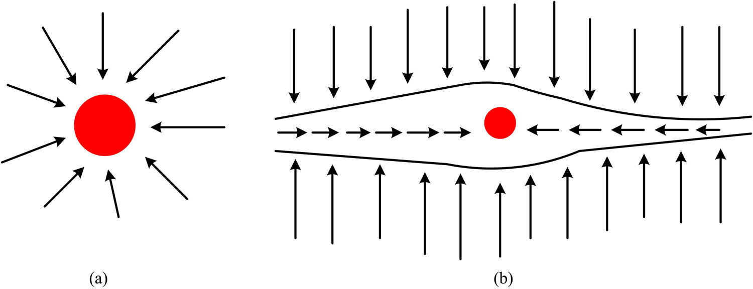
Fluid morphology. (a) Before fracturing and (b) after fracturing.

Figure 2 shows the changes in fluid morphology. In Figure 2(a), the arrow radiates outward from the wellbore, indicating that the fracturing fluid is injected into the formation from the wellbore, forming an initial radial flow. With the injection of fracturing fluid, the formation pressure gradually increases until it exceeds the tensile strength of the rock, leading to the formation of cracks near the wellbore. In Figure 2(b), the arrow shows that the fractured area extends deep into the formation, and the oil and gas flow changes from the original radial flow to a bilinear unidirectional flow. The advantage of this unidirectional flow is that it allows fluid to flow more directly from the reservoir to the wellbore, reducing fluid diffusion and flow around complex pore structures. As a result, compared to before fracturing, the changed linear fluid greatly reduces flow resistance. In addition, communication with oil and gas storage areas is another major reason why this technology can achieve increased production [14]. Due to the heterogeneity of the formation, there is a situation where the oil and gas accumulation zone is not connected to the wellbore. Therefore, artificial fractures formed by fracturing can achieve the connection between natural fractures and artificial fractures. Based on hydraulic fracturing technology, corresponding practical systems can be constructed for the collection of materials such as coal, oil, shale gas, etc., as shown in Figure 3.

Figure 3

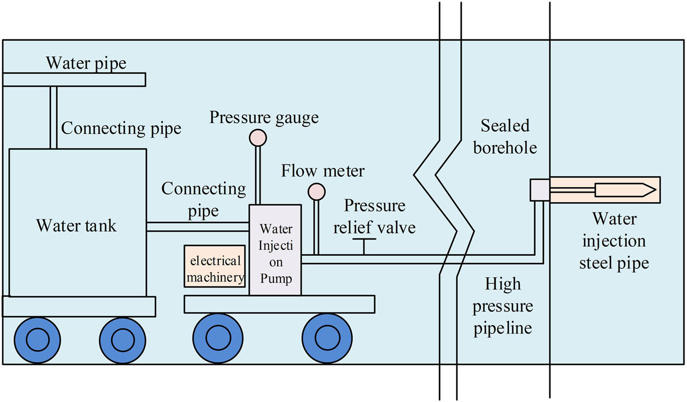
Construction of hydraulic fracturing system.

Figure 3 is a schematic diagram of the system structure constructed based on hydraulic fracturing technology. This figure takes oil collection as an example, from which it can be seen that there are multiple core components in the system, such as water tanks, motors, water injection pumps, and high-pressure pipelines [15]. Among them, the pressure gauge is used to monitor water pressure, while the high-pressure pump provides the high-pressure water flow required for fracturing and injects it into the underground reservoir through drilling. In addition, the water tank can store water resources, the flow meter is used to monitor the flow rate of water, and the use of the pressure relief valve is related to the pressure bearing capacity of the system itself. When the system pressure reaches the release threshold, the entire system will use high-pressure pipelines to connect the water injection steel pipe and ultimately complete the hydraulic fracturing task.

2.2 Tracer technology for hydraulic fracturing radioactive sources based on mechanics models

Although hydraulic fracturing technology is currently the main development technique used for substances such as oil and natural gas, it often faces the dilemma of being unable to describe the formation fractures after use [16]. In order to more accurately explain the specific distribution of underground fractures after hydraulic fracturing, the study adopted the fracturing tracing method, which combines the advantages of hydraulic fracturing and radioactive source tracing technology. Strictly speaking, this technology is a monitoring and evaluation tool. Its main process is to add different energy tracers to the fracturing fluid and pump them into the formation during the fracturing process. Then, the natural gamma ray spectroscopy logging tool is used to measure the gamma count rate around the wellbore, in order to obtain the distribution of proppants, estimate the fracture conductivity, evaluate the segmented fracturing efficiency, and identify the height and distortion of fractures, as shown in Figure 4.

Figure 4

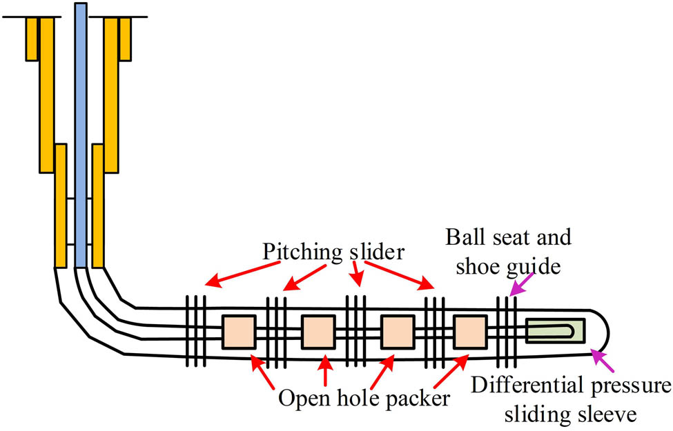
Fracturing horizontal well flow chart.

Figure 4 is a schematic diagram of a fractured horizontal well, which effectively illustrates the specific process of fracturing tracing. From this figure, after drilling is completed, it is necessary to immediately perform segmented perforation on the horizontal well to form fractures. After the crack appears, the grafting fracturing tracer technology can be used. This process usually starts from the inside of the horizontal well and is independently constructed based on the segmented perforation positions. The main function of the pitching slider is to control the flow of fracturing fluid and the opening of the fracturing section [17,18]. In summary, hydraulic fracturing operations will select and deploy spheres of appropriate specifications and materials according to the requirements of different stages. When the spheres reach the designated slider position, they will interact with the sealing components of the slider, changing the slider state and allowing fracturing fluid to flow into the formation fractures. Once the current stage of the operation is completed, the open hole packer will separate the well section where the fracturing fluid injection has been completed from the well section to be injected. After the injection of fracturing fluid into all sections, the tracer dose in each section will vary, providing a basis for subsequent differentiation and evaluation [19,20]. Based on this, the tracer migration in each section of the fracture during the fracturing tracer process can be further divided into three stages: injection, shut in, and backflow, as shown in Figure 5.

Figure 5

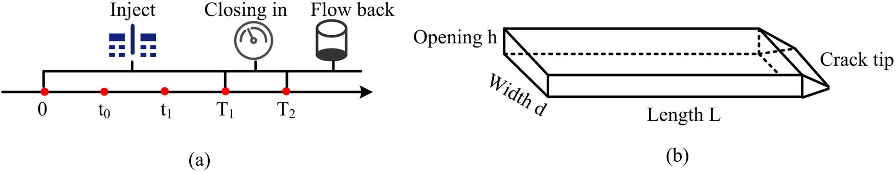
Fracturing tracer timeline and fracture model. (a) Timeline of fracturing tracer process and (b) fracture model.

Figure 5 shows the timeline of the fracturing tracer process and the plate-like fracture model, which is based on a two-dimensional assumption. Among them, Figure 5(a) shows the timeline of the fracturing tracer process, while Figure 5(b) presents a two-dimensional schematic model of the plate-like fracture. The selection of a two-dimensional model is to simplify the analysis while clearly demonstrating the basic characteristics of crack propagation and tracer migration. From Figure 5(a), it can be seen that the time node of tracer migration is bounded by time T ₁, with the 0–T ₁ time period being the injection stage, the T ₁–T ₂ time period being the shut in stage, and the time period greater than T ₂ being the backflow stage [21,22]. In addition, the injection stage from 0–T ₁ can be further subdivided, with t₀ as the time point and the time period from 0–t ₀ as the pre-injection stage, during which there is no tracer present. t ₀–t ₁ is the injection stage of fracturing fluid. In the replacement solution injection stage from t ₁–T ₁, similar to the pre-injection stage, the replacement solution also does not contain tracer. From Figure 5(b), it can be seen that the formed fracture runs through the reservoir, so the width of the fracture is consistent with the thickness of the reservoir, and the tracer can migrate in the positive direction on the coordinates established with the inner boundary of the fracture as the origin [23,24,25]. Based on the above process background, a mechanics model can be established, as shown in Eq. (1).

where C r represents the concentration of tracer adsorption, C represents the concentration of tracer, and a and b are both adsorption constants. The first relation in Eq. (1) represents the expression when the concentration level is high, while the second sub-equation represents the linear expression when the concentration level is low. In addition, D L represents the diffusion mixing coefficient in the direction of seepage, ϒ L means the axial tortuosity of the rock, a L means the diffusion coefficient of the medium, D m represents the one molecule diffusion coefficient, and ϕ represents the rock porosity and the true flow velocity u of the pores. Obviously, in Eq. (1), the third sub-equation is the expression of the mixing coefficient in the direction of tracer flow, while the fourth sub-equation is a simplified linear relationship expression between the dispersion mixing coefficient and pore flow velocity [26,27]. The former is a complete form suitable for general situations, while the latter is a simplified form suitable for high flow velocity conditions dominated by mechanical dispersion. At high flow rates, the molecular diffusion term D m ϒ L ϕ is much smaller than the mechanical diffusion term a L u 1.2 , and u 1.2 can be approximated as u , at which point, the two tend to be consistent. Based on the obtained dispersion mixing coefficient, the mass transfer diffusion velocity u of the tracer can be further obtained, where ∂ c ∂ x represents the concentration gradient of the tracer in the flow direction, c represents the concentration gradient of tracer in the flow direction, used to describe the spatial variation in concentration. Please refer to Figure 6 for details.

Figure 6

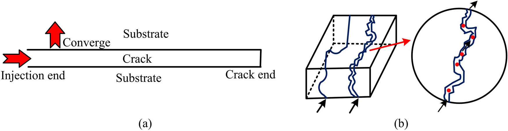
Schematic diagram of tracer flow direction. (a) Cross section view and (b) vertical view.

Figure 6 shows the specific flow direction of tracer in the crack. From this figure, it can be seen that the flow direction of the tracer in the crack starts from the injection end and extends along the direction of the crack, all the way to the end of the crack. During this process, the tracer will flow along with the fluid in the fracture and interact with the fracture wall and the primary fluid in the reservoir during the flow process. Therefore, based on the infiltration effect of tracer transport process, there are still cases where tracer molecules enter the matrix from the crack with water molecules, but overall, the flow path of tracer is from the injection end to the end of the crack.

2.3 Tracer technology for hydraulic fracturing radioactive sources based on improved mechanics models

Although the combination of tracer technology in hydraulic fracturing technology can form a radioactive source tracer technology for hydraulic fracturing, and accurately describe the distribution of underground fractures after hydraulic fracturing based on mechanics models, the current mechanics models for fracturing tracer do not take into account the exchange between fractures and matrix fluids, as well as the stress sensitivity of fractures, and cannot calculate the concentration of fracturing tracer backflow. Thus, it is needful to further improve the mechanics model of the abovementioned hydraulic fracturing radioactive source tracing technology. The prerequisite for improvement is to first construct a basic mechanics model for the convective diffusion of tracer, as shown in Figure 7.

Figure 7

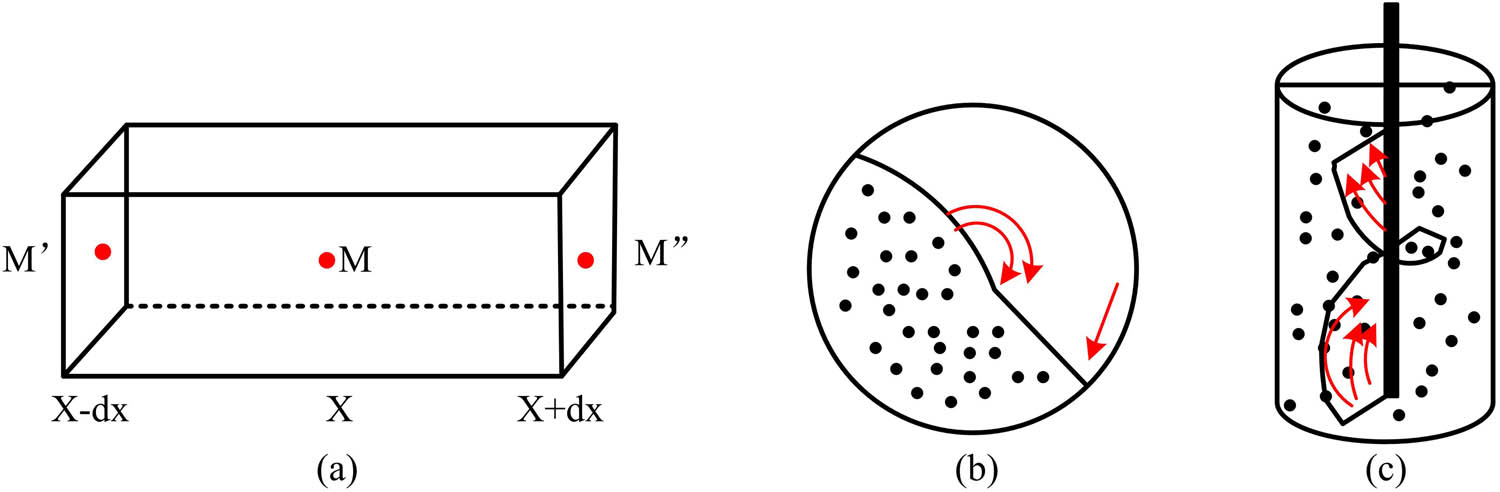
Visualization of convection diffusion. (a) Unit structure, (b) diffuse, and (c) convection.

Figure 7 shows the visualization of the mathematical expression for convective diffusion during tracer transport process. In this figure, X represents the direction of tracer transport, and d x represents the transport distance. M , M ′ , and M ' ' all represent a certain cross-sectional position of tracer transport in the unit cell, where the mass transfer and diffusion velocity of tracer mixing corresponding to point M is U i . Based on the structure of this unit cell, the mass transfer diffusion velocity and flow rate of tracer mixing at point M ' and point M ″ can be calculated correspondingly, as shown in Eq. (2).

where v 1 represents the mass transfer and diffusion velocity of tracer mixing at point M ′ , and y 1 represents the tracer flow rate at the cross-section where the point is located. In addition, v 2 represents the mass transfer and diffusion velocity of tracer mixing at point M ″ , while v 3 represents the mass transfer and diffusion velocity of tracer mixing at that point [28]. U i represents the mass transfer and diffusion velocity of tracer mixing, d x represents the distance of tracer migration, A represents the cross-sectional area, and ϕ f represents the porosity, which is the volume proportion of pores in the rock. S o represents oil saturation, which is the proportion of pores filled with oil. S wc represents water saturation, which is the proportion of pores filled with water. Dt represents a small change in time. Based on the mathematical expression of the unit cell structure, the final mathematical differential equation can be obtained, as shown in Eq. (3).

Eq. (3) is expressed as a general differential equation for tracer convection diffusion, where R represents the retention factor of the crack. According to this differential equation, an optimized mechanics model for hydraulic fracturing radioactive source tracing technology can be constructed by considering both invasion factors and stress sensitivity. The mathematical expression for the migration and diffusion of tracer during the injection process is given in Eq. (4).

where λ 1 represents the invasion factor of the immersion process, and this invasion factor is a non-zero positive number. u i n represents the function of tracer injection rate and time, and C u 1 λ represents the concentration of tracer during the injection process. Furthermore, due to the limited testing period considering external boundary conditions, the tracer cannot migrate to infinity. Therefore, the Dirichlet condition is set based on the actual situation, which means that in the initial state, the formation does not contain any introduced tracer [29]. The obtained convection diffusion equation is shown in Eq. (5).

Eq. (5) represents the mathematical expression of tracer convection diffusion during the injection process, taking into account both invasion factors and stress sensitivity. After the injection stage, there is still a second stage of shut in, and the mathematical expression of tracer convection and diffusion in this stage is Eq. (6).

where T 1 represents the initial moment of wellbore blockage, used to record the initial situation before tracer injection. C u 2 λ ( x , T 1 ) represents the distribution of tracer, that is, the spatial distribution state of tracer in the wellbore or formation at the initial moment. L is the length of the fracture, which directly reflects the scale and extension range of the fracture generated by the fracturing operation in the formation. At this point, the flow velocity of the tracer is zero, and both the inner and outer boundaries are Neumann or Dirichlet conditions with zero gradient or concentration. After the injection and shut in stages, there is still a backflow stage. Therefore, taking into account the invasion factor and stress sensitivity, the mechanics model of tracer convection diffusion in the backflow stage can be expressed as Eq. (7).

Eq. (7) is the mechanics model of the optimized and improved hydraulic fracturing radioactive source tracing technology during the flowback stage. Among them, C u 3 λ represents the tracer concentration function during the reflux process, u re represents the actual flow velocity of the tracer during the reflux process, which is a function of time, and C u 2 λ ( x , T 2 ) represents the tracer distribution during the reflux stage, with the specific time of reflux starting at T 2 . At this point, the invasion factor is a non-zero negative number, and both the inner and outer boundaries are infinite Dirichlet conditions [30,31]. Based on the improved mechanics model, the hydraulic fracturing radiotracer technology can simultaneously consider invasion factors and stress sensitivity.

2.4 Numerical resolution method

The system of partial differential Eqs. (1)–(7) was solved numerically through a carefully designed computational framework. Spatial discretization was implemented using the finite volume method with unstructured grid generation for the fracture domain, where grid sizes were controlled within 0.1–0.5 m to ensure resolution of fracture propagation details. Temporal integration adopted an implicit Euler scheme ( Δ t = 0.01 s ) with Courant number maintained below unity for stability. For the stress-sensitive terms in Eq. (5), the nonlinear system was handled through Newton-Raphson iteration, with convergence achieved when the residual norm fell below 10⁻⁶. Boundary conditions were rigorously implemented: Dirichlet conditions were enforced through direct nodal value assignment, while Neumann conditions were treated via equivalent source term transformation. The resulting linear systems were solved using the GMRES algorithm within a parallel computing architecture built on the PETSc library, enabling efficient large-scale simulations. Numerical accuracy was verified through grid independence tests showing less than 2% variation in key outputs when grid size was reduced beyond the selected parameters.

3.1 Verification and analysis of hydraulic fracturing radioactive source tracing technology based on mechanics models

As the mechanics model for tracer of hydraulic fracturing radioactive sources has been preliminarily established, the mechanics model can be solved and validated to clarify the impact mechanisms of tracer mass transfer diffusion and crack stress sensitivity on tracer concentration. As the new mechanics model is an improvement grounded on the initial mechanics model that did not comprehensively consider invasion factors and stress sensitivity, it can be solved based on the original mechanics model first to verify the correctness of the model solution. The specific results are shown in Figure 8.

Figure 8

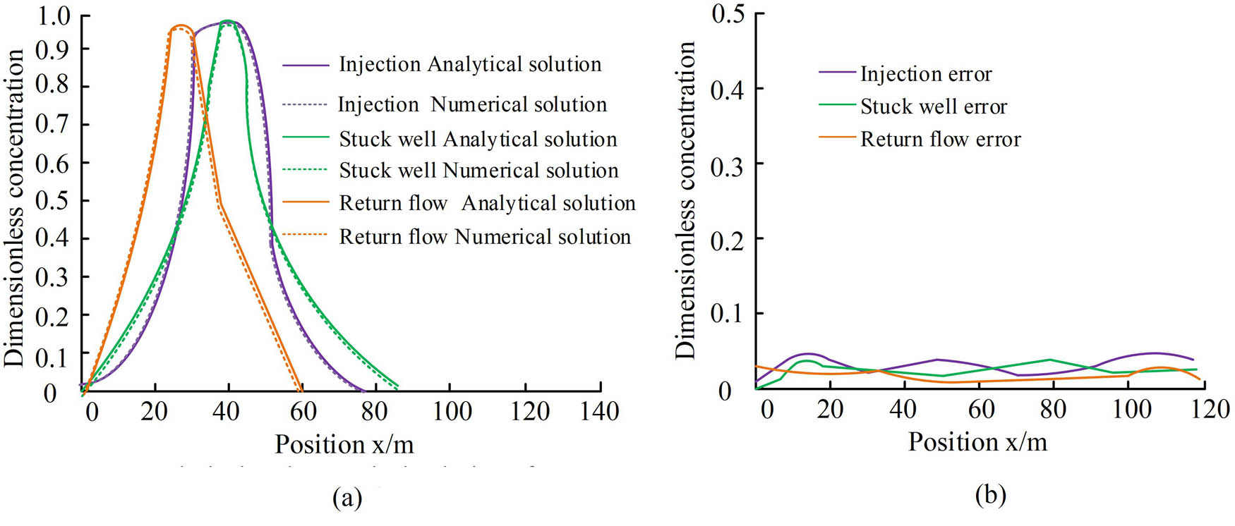
Solutions and error performance of tracer concentration distribution at different stages. (a) Analytical and numerical solutions for tracer concentration at different stages and (b) error function.

Figure 8 shows the numerical solution, analytical solution, and error situation of tracer concentration distribution after the three stages of injection, shut in, and backflow are completed. Analytical solution refers to the exact solution directly obtained using mathematical equations, which is equivalent to the “standard answer,” while numerical solution is the solution obtained through computer approximation calculation. The simultaneous use of both here is to verify the correctness of the model, that is, if the numerical solution and analytical solution match, it indicates that the model is reliable. Figure 8(a) shows the numerical and analytical solutions of tracer concentration distribution after the three stages are completed. From this, in all three stages, the distribution curve of tracer concentration basically followed a normal distribution, with the variance in the backflow stage being lower than that in the injection and shut in stages. In terms of dimensionless concentration, the highest concentration of 1 was reached at position 40 m during the injection stage, while the highest concentration of 0.9 was reached at the same position as the injection stage at 40 m during the shut in stage. However, the highest concentration value at this time was less than 1 during the injection stage. Unlike the previous two stages, the highest concentration of about 0.95 was only reached at position 20 m during the flowback stage. Nevertheless, the three stages maintained a high degree of consistency in their analytical and numerical solutions. Furthermore, from the error situation of tracer concentration distribution in the three stages shown in Figure 8(b), the error values of all three stages were relatively low, and the highest error did not exceed 0.1. Overall, it indicated that the proposed model had correct solutions in solving mechanics models. After verifying the correctness of the basic solution of the model, further impact analysis can be conducted on the proposed model. The experimental synthesis analyzed the tracer retention factor, invasion factor, and crack stress sensitivity of the model separately. The specific situation of tracer retention factor is shown in Figure 9.

Figure 9

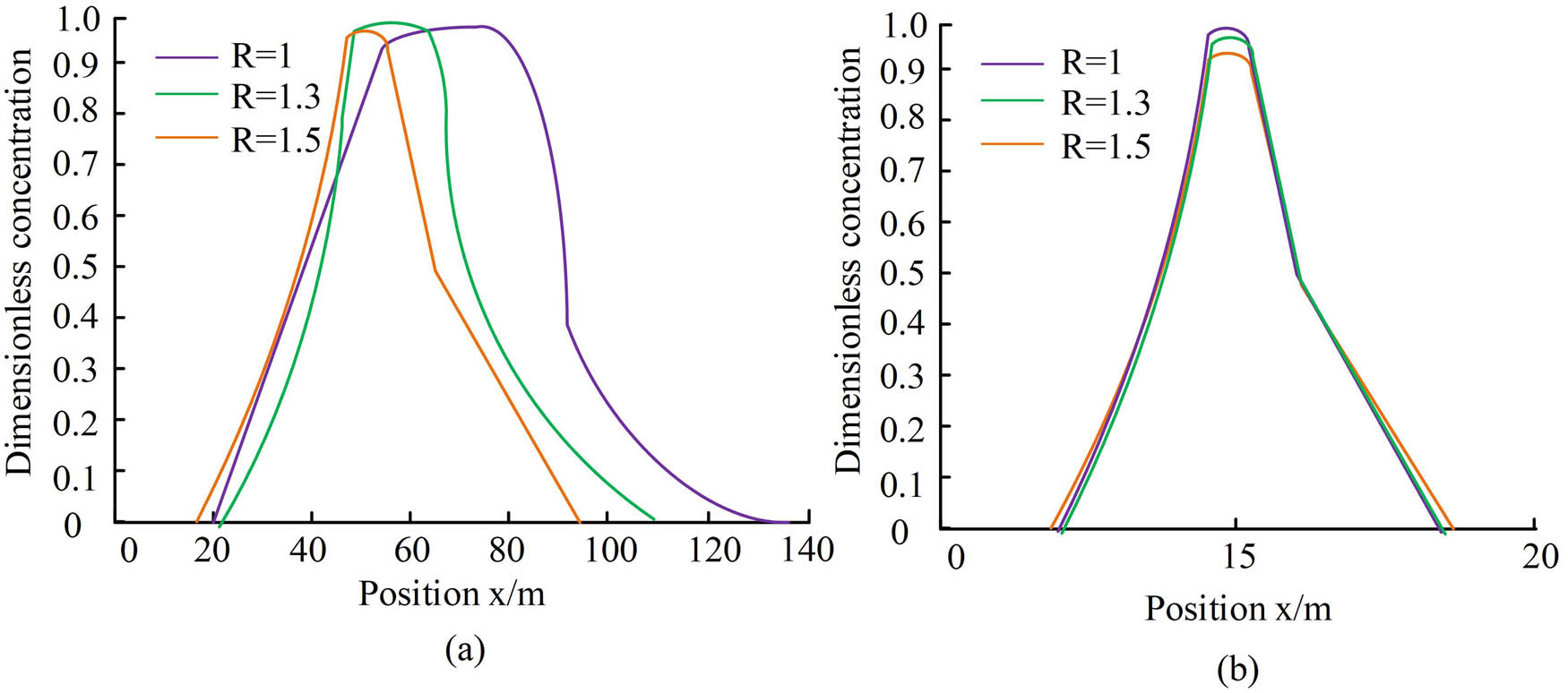
Analysis of the influence of tracer retention factor. (a) The injection process of different blocking factors ends with dimensionless concentration distribution of tracer and (b) non-dimensionless concentration flowback curves of tracer agents with different blocking factors.

Figure 9 shows the analysis results of the impact of tracer retention factors on the mechanics model constructed for the research. Figure 9(a) shows the dimensionless concentration distribution of tracer with respect to position under various retention factor conditions at different stages. From this, the size of the retention factor did not affect the high-low distribution of tracer dimensionless concentration during the injection stage, but rather affected the position and concentration of each concentration distribution. Specifically, the larger the retention factor, the higher the dimensionless concentration of the tracer, resulting in a more concentrated concentration distribution. Figure 9(b) shows the dimensionless concentration distribution of tracer after the end of reflux for retention factors of different sizes. Unlike the injection stage, the size of the retention factor in the reflux stage did not affect the position and concentration of the curve, but only changed the high-low distribution of dimensionless concentrations. That is to say, regardless of the retention factor of the formation, it did not affect the time when the dimensionless concentration peak of the tracer appears during the backflow stage. The analysis results of the impact of tracer invasion factors can be seen in Figure 10.

Figure 10

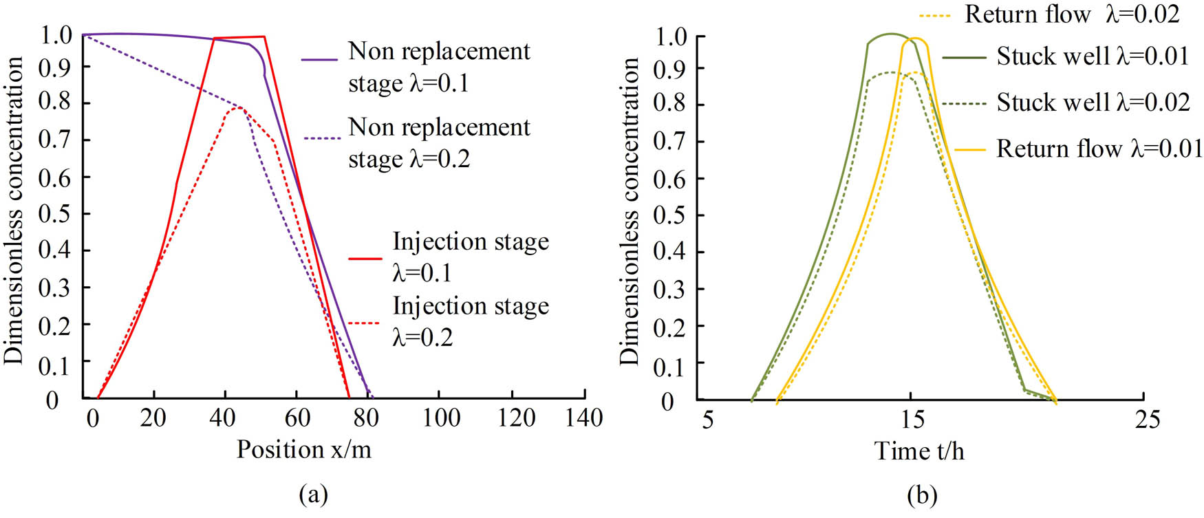
Analysis of the impact of tracer invasion factors. (a) Non-dimensional concentration flowback curves of tracer during the non-replacement and injection stages of different invasion factors and (b) non-dimensional concentrations of tracer agents during different invasion factors, well plugging, and backflow stages.

Figure 10 indicates the analysis of the impact of tracer invasion factors. Figure 10(a) indicates the dimensionless concentration curves of tracer agents with different sizes of invasion factors during the non-replacement and injection completion stages, which are a function of position and concentration. Among them, the non-replacement stage is the stage of sand carrying fluid injection before the injection stage. From this figure, if the invasion factor was 0, the tracer concentration remained basically the same as before injection, and it infiltrated the crack with almost unchanged concentration values. However, as the invasion factor increased, the concentration value of the tracer penetrating the crack rapidly decreased, but the overall range remained unchanged. In addition, the dimensionless concentration curve of the tracer at the end of injection stage showed a similar trend to the non-displaced stage. Figure 10(b) shows the concentration curves of invasion factors of different sizes during the shut in and backflow stages, which are functions of time and concentration. From the graph, the size of the invasion factor did not affect the distribution time of shut in and backflow, but only affected the size of the concentration peak. However, to a greater extent, the peak size during the shut in stage varied more with the invasion factor, while the amplitude of this change was slightly weaker during the backflow stage. The results of the stress sensitivity analysis of cracks are shown in Figure 11.

Figure 11

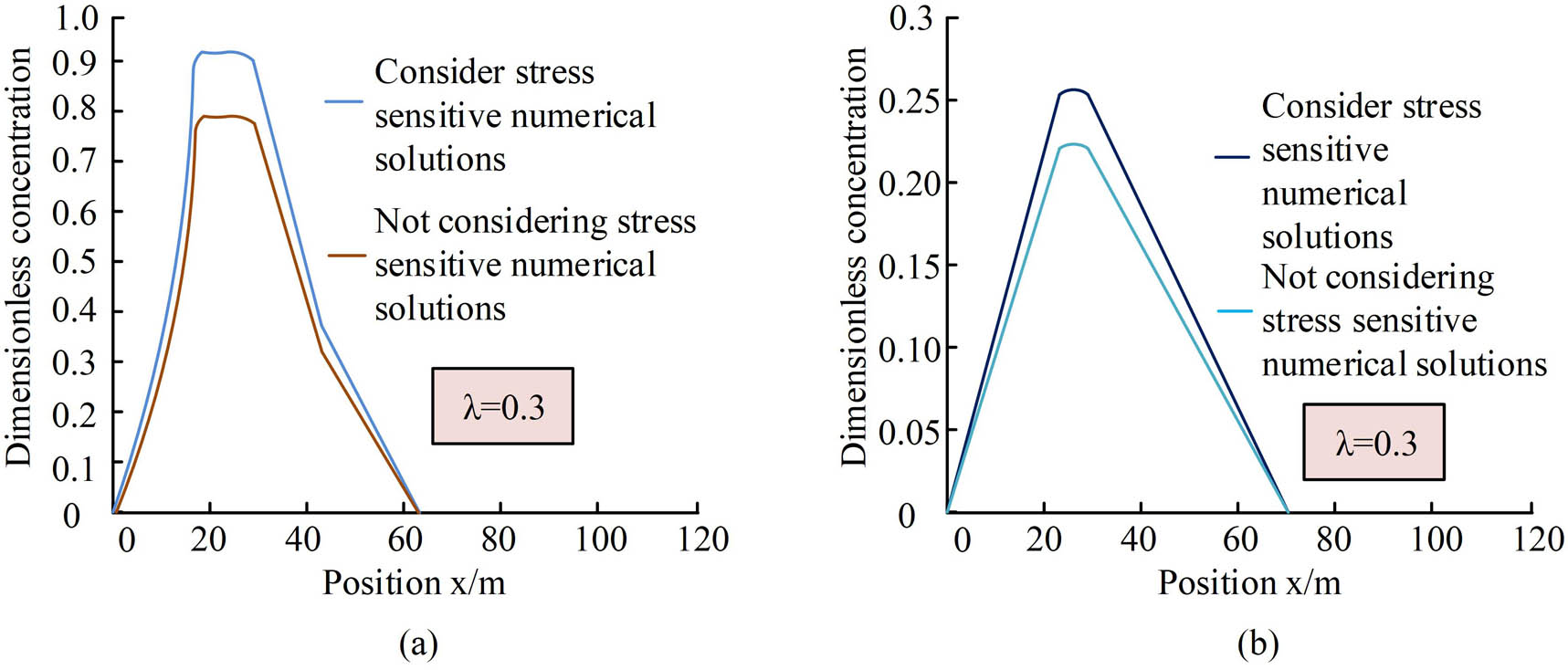
Analysis of stress sensitivity effects of cracks. (a) Consideration and non-consideration of stress sensitive injection end tracer dimensionless concentration distribution and (b) consider and ignore stress sensitive confinement end tracer dimensionless concentration distribution.

Figure 11 shows the analysis results of the stress sensitivity of fractures during the injection stage and the shut in stage. Figure 11(a) indicates the dimensionless concentration distribution of tracer before and after considering stress sensitivity during the injection stage, while Figure 11(b) indicates the dimensionless concentration distribution of tracer before and after considering stress sensitivity during the shut in stage. From the comparison of the two graphs, compared to not considering stress sensitivity, the curve that considered stress sensitivity showed varying degrees of peak drop. In order to further verify the accuracy of the proposed model, a comparative analysis was conducted by combining actual fracturing data from a certain oil field. Two fracturing wells (A well and B well) in the same block were selected for the experiment, with A well using traditional tracing methods and B well using the optimized mechanics model proposed by the research institute for tracing analysis. The specific results are shown in Table 1.

Table 1 shows the performance comparison between the optimized model and traditional methods. It can be seen from the table that the optimized model exhibits significant advantages in various key indicators. In terms of the fitting error of tracer reflux concentration, the optimized model reduced the error from 22.5% in traditional methods to 10.5%, with a decrease of 12% in error. In predicting the direction of crack propagation, the consistency based on microseismic monitoring data increased from 73 to 85%, and the accuracy improved by 12 percentage points. In terms of production capacity prediction, the error of oil production prediction has been reduced from ±18.7 to ±9.3%, and the error range has significantly narrowed. In addition, the prediction error of tracer peak time during the flowback stage decreased from ±4.2 to ±1.8 h, and the time prediction accuracy improved by 2.4 h. This indicates that the optimized model has significant advantages in tracer dynamic analysis, crack propagation prediction, and productivity evaluation.

3.2 Case analysis of tracer technology for hydraulic fracturing radioactive sources based on mechanics models

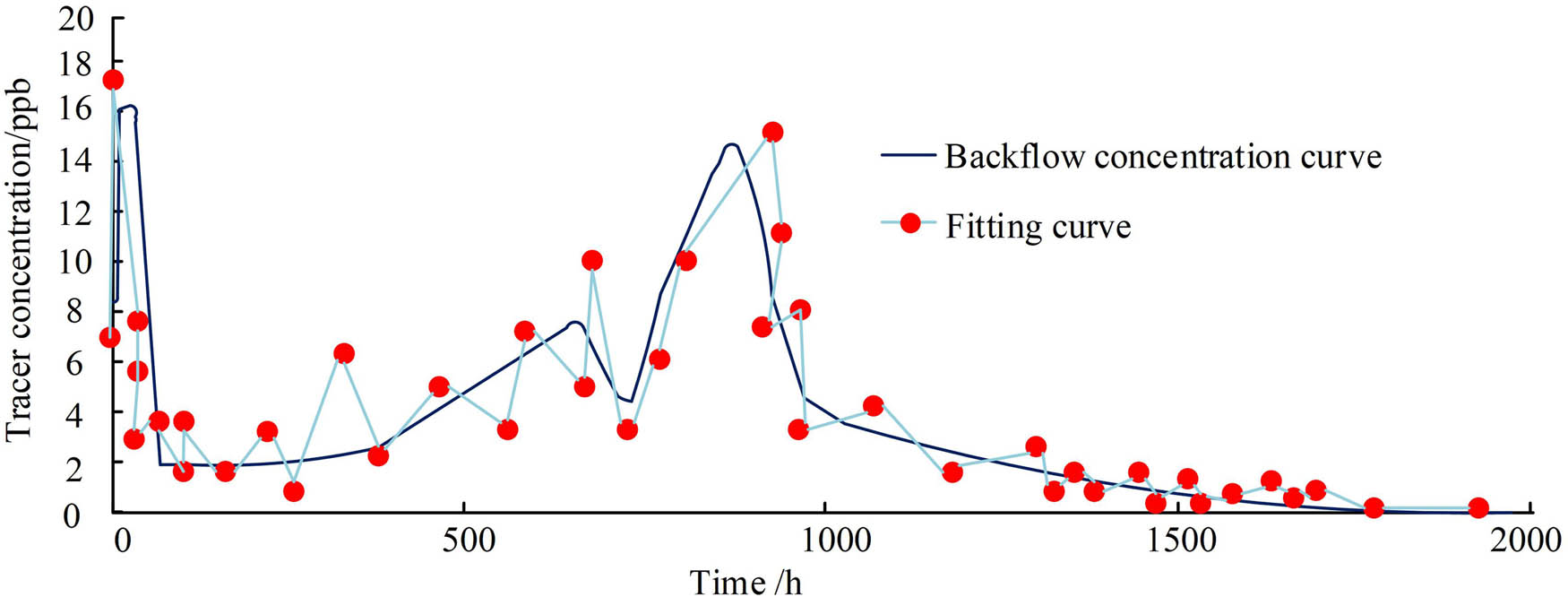
The above is an analysis of the impact mechanism of the model. To more intuitively demonstrate the advantage of the proposed model, the experiment further conducted an example analysis. Using a hydraulic fracturing well in a certain experimental area as the experimental object, on-site monitoring was conducted using the model proposed by the research. Oil tracer was selected as the tracer, and the backflow concentration curve and fitting curve of the fracturing tracer were plotted, as shown in Figure 12.

Figure 12

Fracturing tracer backflow and fitting curve.

Figure 12 shows the flowback curve and fitting curve of the fracturing tracer. From this curve, it can be preliminarily inferred that due to the presence of three peaks, there were three fractures in the hydraulic fracturing well in this experimental area. After careful observation, it was found that the first peak curve had a parabolic shape, indicating that the crack belonged to a high conductivity channel containing branching cracks. The second peak curve shows a non-standard normal distribution, so it can be considered as a micro crack. The third peak curve shows a clear normal distribution, indicating that this crack belongs to a high conductivity channel without branching cracks. In addition, the specific parameter values used to determine the fitting effect after fitting have a variance of 148.9, a coefficient of determination of 0.81, and a root mean square error (RMSE) of 1.87, indicating a good fitting situation. Furthermore, the study compared the experimental values with the actual on-site conditions and found that the two situations were consistent. Based on this, the experiment will conduct productivity testing on a certain section of the oil field in the experimental area. To demonstrate the superiority of the proposed model more intuitively, the unoptimized model was included as a comparative model, and the outcomes are shown in Figure 13.

Figure 13

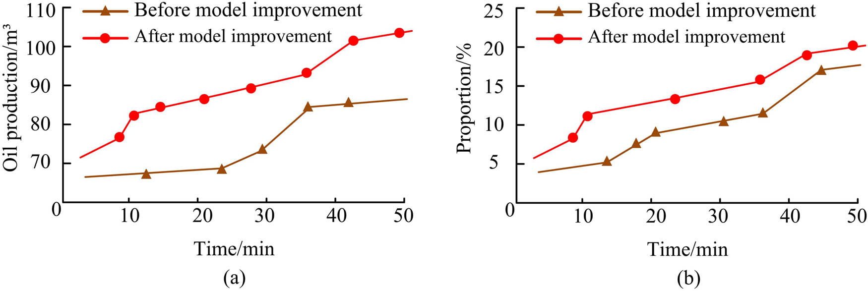
Oil field productivity before and after improvement. (a) Oil production situation and (b) proportion of oil production.

Figure 13 shows the specific production capacity of the experimental oilfield before and after model improvement. From the table, before the model improvement, the oil production was 87.3 m³, and the proportion of oil production in the experimental section in this area was 17.1%. After the model was improved, the oil production of the experimental section was 104.2 m³, with an increase of 16.9 m³ in oil production. In addition, the oil production ratio of the experimental section corresponding to the improved model in the original area was 20.4%, an increase of 3.3%, indicating that the improved model can improve production capacity. In addition, water solubility tracing was further monitored, and the water contribution rate of the model is shown in Figure 14.

Figure 14

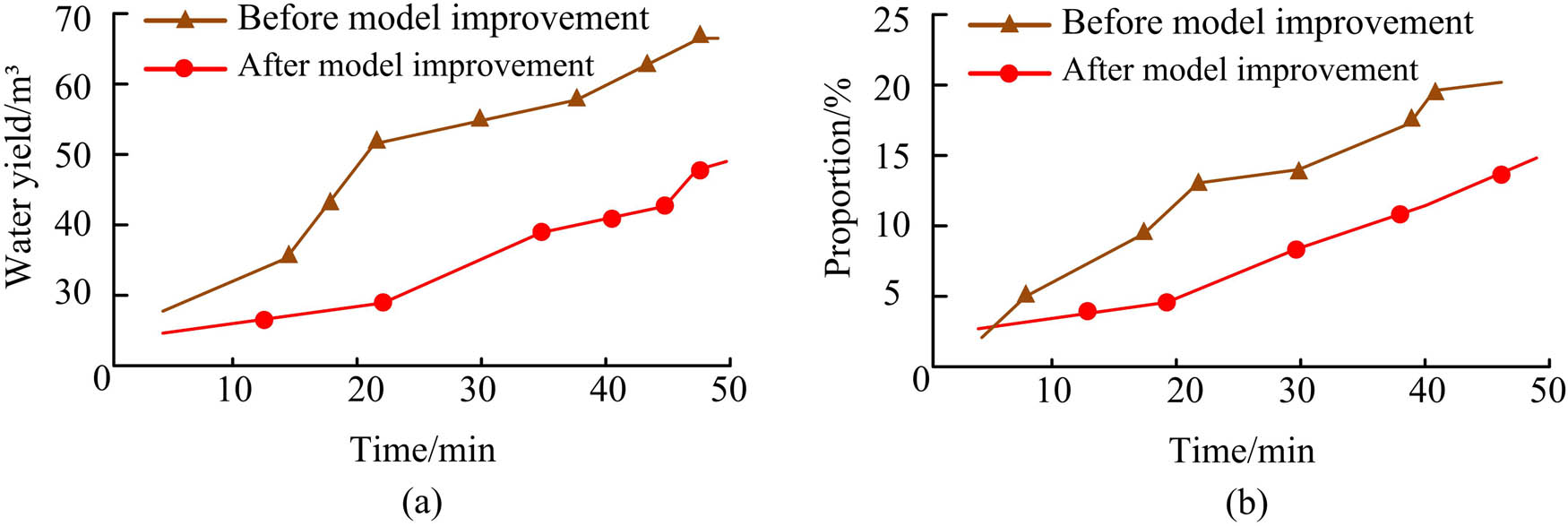
Water production situation in the experimental section. (a) Water yield situation and (b) water occupancy rate performance.

Figure 14 shows the specific water production situation of the experimental oilfield 1 before and after model improvement. From this table, before the model improvement, the specific water production was about 68.5 m³, accounting for 21.3% of the total water production. After the model was improved, the water production of the experimental section was 47.6 m³, accounting for 15.8% of the total water. Compared with before the improvement, the improved model has a 20.9 m³ lower water production and a 4.5% lower water proportion. Due to the fact that the oil field in this section was in the low water cut oil recovery period during the experiment, and the water content during the low water cut period is usually 2–20%, if the water content is low at this time, it means that the production capacity and extraction efficiency of the oil well in this section are high. Obviously, compared to before the improvement, the improved model had lower water production and water occupancy rate, resulting in higher mining efficiency. Based on this, the experiment further compared the economic and environmental benefits of the two models before and after, as shown in Figure 15.

Figure 15

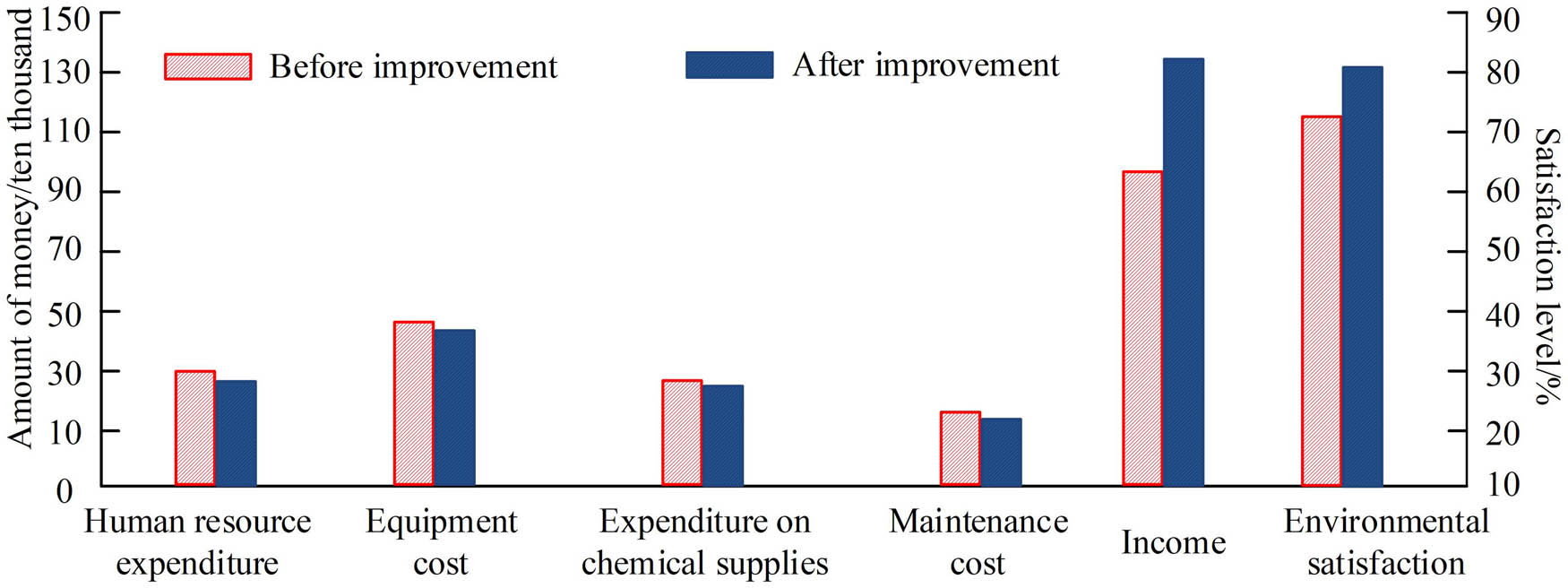
Economic and environmental benefits of the model.

Figure 15 shows the economic and environmental benefits before and after model improvement. From the graph, in terms of manpower expenditure, a fixed monthly expenditure of about 300,000 yuan was required before the improvement, but after the improvement, there was a slight decrease of about 292,000 yuan in manpower expenditure. In terms of equipment cost, the monthly expenditure before the improvement was 489,000 yuan, but after the improvement, it decreased by 97,000 yuan, only 392,000 yuan. In terms of expenditure on the use of chemical products, the model required 243,000 yuan before improvement and 217,000 yuan after improvement, a decrease of 26,000 yuan. In terms of maintenance costs, it was 100,000 before the improvement and 98,000 after the improvement. In terms of revenue, the original revenue was 1.01 million per month, and the improved revenue could reach 1.34 million. In addition, in terms of environmental benefits, the overall environmental satisfaction before improvement was only 73.2%, while after improvement, the overall environmental satisfaction increased to 81.4%. Overall, the model proposed by the research performs better in terms of both economic and environmental benefits.

References

[1] Heider Y. A review on phase-field modeling of hydraulic fracturing. Eng Fract Mech. 2021;253:107881.10.1016/j.engfracmech.2021.107881Search in Google Scholar
[2] Wu Z, Cui C, Jia P, Zhen W, Sui Y. Advances and challenges in hydraulic fracturing of tight reservoirs: A critical review. Energy Geosci. 2022;3:427–35.10.1016/j.engeos.2021.08.002Search in Google Scholar
[3] Du D, Hao F, Li Y, Li D, Tang Y. Study on interpretation method of multistage fracture tracer flowback curve in tight oil reservoirs. ACS Omega. 2024;9:11628–36.10.1021/acsomega.3c08411Search in Google Scholar PubMed PubMed Central
[4] Liu S, Du H, Tian J, Zhang Y, Liu J, Tian X, et al. Study on an anti-adsorption micromaterial tracer system and its application in fracturing horizontal wells of coal reservoirs. ACS Omega. 2023;8:28821–33.10.1021/acsomega.3c03773Search in Google Scholar PubMed PubMed Central
[5] Hua C, Jiang Z, Li J, Xu J, Lei Y, Zhu H. Tracer-test-based dimensionality reduction model for characterizing fracture network and predicting flow and transport in fracture aquifer. J Hydrol. 2024;630:130773–4.10.1016/j.jhydrol.2024.130773Search in Google Scholar
[6] Jing C, Duan Q, Han G, Nie J, Li L, Ge M. Quantitative interpretation model of interwell tracer for fracture-cavity reservoir based on fracture-cavity configuration. Process. 2023;11:964–5.10.3390/pr11030964Search in Google Scholar
[7] Gong Z, Li N, Kang W, Qin M, Wu Y, Liu X. Novel oleophilic tracer-slow-released proppant for monitoring the oil production contribution. Fuel. 2024;364(1):130945.10.1016/j.fuel.2024.130945Search in Google Scholar
[8] Luan Y, Hao P, Cao G, Liu J. Crack propagation during the process of carbon dioxide fracturing based on molecular dynamics simulations. Energy Fuels. 2023;37:1022–32.10.1021/acs.energyfuels.2c03552Search in Google Scholar
[9] Yu H, Xu WL, Li B, Huang H, Micheal M, Wang Q, et al. Hydraulic fracturing and enhanced recovery in shale reservoirs: Theoretical analysis to engineering applications. Energy Fuel. 2023;37:9956–97.10.1021/acs.energyfuels.3c01029Search in Google Scholar
[10] Xue Y, Liu S, Chai J, Liu J, Ranjith PG, Cai C, et al. Effect of water-cooling shock on fracture initiation and morphology of high-temperature granite: Application of hydraulic fracturing to enhanced geothermal systems. Appl Energy. 2023;337:120858.10.1016/j.apenergy.2023.120858Search in Google Scholar
[11] Zhuang L, Zang A. Laboratory hydraulic fracturing experiments on crystalline rock for geothermal purposes. Earth-Sci Rev. 2021;216:103580.10.1016/j.earscirev.2021.103580Search in Google Scholar
[12] Davoodi S, Al-Shargabi M, Wood DA, Valeriy SR. A comprehensive review of beneficial applications of viscoelastic surfactants in wellbore hydraulic fracturing fluids. Fuel. 2023;338:127228.10.1016/j.fuel.2022.127228Search in Google Scholar
[13] Jew AD, Druhan JL, Ihme M, Anthony RK, Lienia B, John PK, et al. Chemical and reactive transport processes associated with hydraulic fracturing of unconventional oil/gas shales. Chem Rev. 2022;122:9198–263.10.1021/acs.chemrev.1c00504Search in Google Scholar PubMed
[14] Zhong C, Zolfaghari A, Hou D, Goss G, Lanoil B, Gehman J, et al. Comparison of the hydraulic fracturing water cycle in China and North America: A critical review. Environ Sci Technol. 2021;55:7167–85.10.1021/acs.est.0c06119Search in Google Scholar PubMed
[15] Guo T, Tang S, Liu S, Liu S, Xu J, Qi N, et al. Physical simulation of hydraulic fracturing of large-sized tight sandstone outcrops. SPE J. 2021;26:372–93.10.2118/204210-PASearch in Google Scholar
[16] Du J, Liu J, Zhao L, Liu P, Chen X, Wang Q, et al. Water-soluble polymers for high-temperature resistant hydraulic fracturing: A review. J Nat Gas Sci Eng. 2022;104:104673.10.1016/j.jngse.2022.104673Search in Google Scholar
[17] Xu S, Guo J, Feng Q, Ren G, Li Y, Wang S. Optimization of hydraulic fracturing treatment parameters to maximize economic benefit in tight oil. Fuel. 2022;329:125329.10.1016/j.fuel.2022.125329Search in Google Scholar
[18] Wang D, Dong Y, Sun D, Bo Y. A three-dimensional numerical study of hydraulic fracturing with degradable diverting materials via CZM-based FEM. Eng Fract Mech. 2020;237:107251.10.1016/j.engfracmech.2020.107251Search in Google Scholar
[19] Zhang L, Hascakir B. A review of issues, characteristics, and management for wastewater due to hydraulic fracturing in the US. J Petrol Sci Eng. 2021;202:108536.10.1016/j.petrol.2021.108536Search in Google Scholar
[20] Sun S, Zhou M, Lu W, Davarpanah AS. Application of symmetry law in numerical modeling of hydraulic fracturing by finite element method. Symmetry. 2020;12:1122.10.3390/sym12071122Search in Google Scholar
[21] Mou P, Pan J, Wang K, Wei J, Yang Y, Wang X. Influences of hydraulic fracturing on microfractures of high-rank coal under different in-situ stress conditions. Fuel. 2021;287:119566.10.1016/j.fuel.2020.119566Search in Google Scholar
[22] Jamaloei BY. A critical review of common models in hydraulic-fracturing simulation: A practical guide for practitioners. Theor Appl Fract Mech. 2021;113(1):102937.10.1016/j.tafmec.2021.102937Search in Google Scholar
[23] Yazdan MMS, Ahad MT, Jahan I, Mozammel M. Review on the evaluation of the impacts of wastewater disposal in hydraulic fracturing industry in the United States. Technologies. 2020;8(4):67.10.3390/technologies8040067Search in Google Scholar
[24] Moska R, Labus K, Kasza P. Hydraulic fracturing in enhanced geothermal systems—field, tectonic and rock mechanics conditions—a review. Energy. 2021;14(18):5725.10.3390/en14185725Search in Google Scholar
[25] Tan P, Chen Z, Fu S, Qing Z. Experimental investigation on fracture growth for integrated hydraulic fracturing in multiple gas bearing formations. Geoenergy Sci Eng. 2023;231:212316.10.1016/j.geoen.2023.212316Search in Google Scholar
[26] Zhang JN, Yu H, Xu WL, Chengsi L, Marembo M, Fang S, et al. A hybrid numerical approach for hydraulic fracturing in a naturally fractured formation combining the XFEM and phase-field model. Eng Fract Mech. 2022;271(1):108621.10.1016/j.engfracmech.2022.108621Search in Google Scholar
[27] Zheng P, Xia Y, Yao T, Jiang X, Xiao P, He Z, et al. Formation mechanisms of hydraulic fracture network based on fracture interaction. Energy. 2022;243(1):123057.10.1016/j.energy.2021.123057Search in Google Scholar
[28] Zhou ZL, Hou ZK, Guo YT, Zhao H, Wang D, Qiu GZ, et al. Experimental study of hydraulic fracturing for deep shale reservoir. Eng Fract Mech. 2024;307(1):110259.10.1016/j.engfracmech.2024.110259Search in Google Scholar
[29] Zhu X, Feng C, Cheng P, Wang X, Li S. A novel three-dimensional hydraulic fracturing model based on continuum–discontinuum element method. Comput Methods Appl Mech Eng. 2021;383(1):113887.10.1016/j.cma.2021.113887Search in Google Scholar
[30] Lin Y, Wang X, Ma J, Huang L. A finite-discrete element based approach for modelling the hydraulic fracturing of rocks with irregular inclusions. Eng Fract Mech. 2022;261(1):108209.10.1016/j.engfracmech.2021.108209Search in Google Scholar
[31] Reynolds MA. A technical playbook for chemicals and additives used in the hydraulic fracturing of shales. Energy Fuel. 2020;34(12):15106–25.10.1021/acs.energyfuels.0c02527Search in Google Scholar
[32] Yang H, Guo K, Lin L, Zhang S, Wang Y. Application of micro-substance tracer test in fractured horizontal wells. J Pet Explor Prod Technol. 2024;14:1235–46.10.1007/s13202-024-01765-zSearch in Google Scholar
[33] Brown NM, Dejam M. Tracer dispersion due to non-Newtonian fluid flows in hydraulic fractures with different geometries and porous walls. J Hydrol. 2023;622:129644.10.1016/j.jhydrol.2023.129644Search in Google Scholar
© 2025 the author(s), published by De Gruyter
This work is licensed under the Creative Commons Attribution 4.0 International License.
Articles in the same Issue
- Research Articles
- Single-step fabrication of Ag2S/poly-2-mercaptoaniline nanoribbon photocathodes for green hydrogen generation from artificial and natural red-sea water
- Abundant new interaction solutions and nonlinear dynamics for the (3+1)-dimensional Hirota–Satsuma–Ito-like equation
- A novel gold and SiO2 material based planar 5-element high HPBW end-fire antenna array for 300 GHz applications
- Explicit exact solutions and bifurcation analysis for the mZK equation with truncated M-fractional derivatives utilizing two reliable methods
- Optical and laser damage resistance: Role of periodic cylindrical surfaces
- Numerical study of flow and heat transfer in the air-side metal foam partially filled channels of panel-type radiator under forced convection
- Water-based hybrid nanofluid flow containing CNT nanoparticles over an extending surface with velocity slips, thermal convective, and zero-mass flux conditions
- Dynamical wave structures for some diffusion--reaction equations with quadratic and quartic nonlinearities
- Solving an isotropic grey matter tumour model via a heat transfer equation
- Study on the penetration protection of a fiber-reinforced composite structure with CNTs/GFP clip STF/3DKevlar
- Influence of Hall current and acoustic pressure on nanostructured DPL thermoelastic plates under ramp heating in a double-temperature model
- Applications of the Belousov–Zhabotinsky reaction–diffusion system: Analytical and numerical approaches
- AC electroosmotic flow of Maxwell fluid in a pH-regulated parallel-plate silica nanochannel
- Interpreting optical effects with relativistic transformations adopting one-way synchronization to conserve simultaneity and space–time continuity
- Modeling and analysis of quantum communication channel in airborne platforms with boundary layer effects
- Theoretical and numerical investigation of a memristor system with a piecewise memductance under fractal–fractional derivatives
- Tuning the structure and electro-optical properties of α-Cr2O3 films by heat treatment/La doping for optoelectronic applications
- High-speed multi-spectral explosion temperature measurement using golden-section accelerated Pearson correlation algorithm
- Dynamic behavior and modulation instability of the generalized coupled fractional nonlinear Helmholtz equation with cubic–quintic term
- Study on the duration of laser-induced air plasma flash near thin film surface
- Exploring the dynamics of fractional-order nonlinear dispersive wave system through homotopy technique
- The mechanism of carbon monoxide fluorescence inside a femtosecond laser-induced plasma
- Numerical solution of a nonconstant coefficient advection diffusion equation in an irregular domain and analyses of numerical dispersion and dissipation
- Numerical examination of the chemically reactive MHD flow of hybrid nanofluids over a two-dimensional stretching surface with the Cattaneo–Christov model and slip conditions
- Impacts of sinusoidal heat flux and embraced heated rectangular cavity on natural convection within a square enclosure partially filled with porous medium and Casson-hybrid nanofluid
- Stability analysis of unsteady ternary nanofluid flow past a stretching/shrinking wedge
- Solitonic wave solutions of a Hamiltonian nonlinear atom chain model through the Hirota bilinear transformation method
- Bilinear form and soltion solutions for (3+1)-dimensional negative-order KdV-CBS equation
- Solitary chirp pulses and soliton control for variable coefficients cubic–quintic nonlinear Schrödinger equation in nonuniform management system
- Influence of decaying heat source and temperature-dependent thermal conductivity on photo-hydro-elasto semiconductor media
- Dissipative disorder optimization in the radiative thin film flow of partially ionized non-Newtonian hybrid nanofluid with second-order slip condition
- Bifurcation, chaotic behavior, and traveling wave solutions for the fractional (4+1)-dimensional Davey–Stewartson–Kadomtsev–Petviashvili model
- New investigation on soliton solutions of two nonlinear PDEs in mathematical physics with a dynamical property: Bifurcation analysis
- Mathematical analysis of nanoparticle type and volume fraction on heat transfer efficiency of nanofluids
- Creation of single-wing Lorenz-like attractors via a ten-ninths-degree term
- Optical soliton solutions, bifurcation analysis, chaotic behaviors of nonlinear Schrödinger equation and modulation instability in optical fiber
- Chaotic dynamics and some solutions for the (n + 1)-dimensional modified Zakharov–Kuznetsov equation in plasma physics
- Fractal formation and chaotic soliton phenomena in nonlinear conformable Heisenberg ferromagnetic spin chain equation
- Single-step fabrication of Mn(iv) oxide-Mn(ii) sulfide/poly-2-mercaptoaniline porous network nanocomposite for pseudo-supercapacitors and charge storage
- Novel constructed dynamical analytical solutions and conserved quantities of the new (2+1)-dimensional KdV model describing acoustic wave propagation
- Tavis–Cummings model in the presence of a deformed field and time-dependent coupling
- Spinning dynamics of stress-dependent viscosity of generalized Cross-nonlinear materials affected by gravitationally swirling disk
- Design and prediction of high optical density photovoltaic polymers using machine learning-DFT studies
- Robust control and preservation of quantum steering, nonlocality, and coherence in open atomic systems
- Coating thickness and process efficiency of reverse roll coating using a magnetized hybrid nanomaterial flow
- Dynamic analysis, circuit realization, and its synchronization of a new chaotic hyperjerk system
- Decoherence of steerability and coherence dynamics induced by nonlinear qubit–cavity interactions
- Finite element analysis of turbulent thermal enhancement in grooved channels with flat- and plus-shaped fins
- Modulational instability and associated ion-acoustic modulated envelope solitons in a quantum plasma having ion beams
- Statistical inference of constant-stress partially accelerated life tests under type II generalized hybrid censored data from Burr III distribution
- On solutions of the Dirac equation for 1D hydrogenic atoms or ions
- Entropy optimization for chemically reactive magnetized unsteady thin film hybrid nanofluid flow on inclined surface subject to nonlinear mixed convection and variable temperature
- Stability analysis, circuit simulation, and color image encryption of a novel four-dimensional hyperchaotic model with hidden and self-excited attractors
- A high-accuracy exponential time integration scheme for the Darcy–Forchheimer Williamson fluid flow with temperature-dependent conductivity
- Novel analysis of fractional regularized long-wave equation in plasma dynamics
- Development of a photoelectrode based on a bismuth(iii) oxyiodide/intercalated iodide-poly(1H-pyrrole) rough spherical nanocomposite for green hydrogen generation
- Investigation of solar radiation effects on the energy performance of the (Al2O3–CuO–Cu)/H2O ternary nanofluidic system through a convectively heated cylinder
- Quantum resources for a system of two atoms interacting with a deformed field in the presence of intensity-dependent coupling
- Studying bifurcations and chaotic dynamics in the generalized hyperelastic-rod wave equation through Hamiltonian mechanics
- A new numerical technique for the solution of time-fractional nonlinear Klein–Gordon equation involving Atangana–Baleanu derivative using cubic B-spline functions
- Interaction solutions of high-order breathers and lumps for a (3+1)-dimensional conformable fractional potential-YTSF-like model