Creation of single-wing Lorenz-like attractors via a ten-ninths-degree term
-
 ,
,
,
,

Abstract
In light of the subtle connection between the strange attractors and the degree of dynamical systems, in this study, we propose a new simple asymmetric Lorenz-like system and report the finding of single-wing Lorenz-like attractors, which can also be created by the collapse of asymmetric singularly degenerate heteroclinic cycles. Moreover, we prove the existence of a single heteroclinic orbit to the origin and the nontrivial equilibrium point. Besides, numerical simulations also verify the theoretical analysis.
1 Introduction
As early as 1990, Cox introduced an asymmetric perturbation of the Lorenz system and illustrated the transition to complicated dynamics in parameter-space, i.e., the classic Lorenz system with a constant
On the one hand, the controlled Lorenz, Chen, and Lü systems are potential candidates that can generate single-wing Lorenz-like attractors, due to the cause of a constant controller. On the other hand, if the constant controller
Researchers have extensively investigated the relationship between polynomial degrees and complex dynamics, particularly in systems exhibiting Lorenz-like attractors and singular orbits. In 2007, replacing
However, now the question is: how to create single-wing Lorenz-like attractors through changing the degrees of state variables, if they exist? To the best of our knowledge, scholars seldom consider this topic. More importantly, studying such a system may shed light on the research hotspot, i.e., data-driven predictions of the chaotic system [18–21]. To achieve this target, by increasing the degree of the linear term
Creating single-wing Lorenz-like attractors by a ten-ninths-degree term.
Explaining the formation of single-wing Lorenz-like attractors through collapses of asymmetric SDHC.
Establishing the existence of a heteroclinic orbit connecting
This proposed quadratic Lorenz-like system aligns with the third principle of Sprott [22], representing the Lorenz-like analogue with only six terms. It addresses a critical gap in traditional Lorenz-like models by leveraging fractional-degree nonlinearity to generate asymmetric dynamics. Unlike controlled Lorenz/Chen systems, which rely on constant perturbations, our model uses a ten-ninths-degree term
The remainder of this work is structured as follows. Section 2 details the construction of the new simple asymmetric Lorenz-like system and reports the main results. Section 3 rigorously demonstrates the presence of a single heteroclinic orbit to
2 New Lorenz-like system and key results
By comparing those Lorenz-like systems [10– 13,15–17] and systematic experimentation, this section first introduces the following new asymmetric Lorenz-like system:
where
Theorem 2.1
Table 4 lists the local behaviors of
Equilibrium points
|
|
|
Distribution of equilibria |
|---|---|---|
|
|
|
|
|
|
|
|
|
|
|
Local dynamics of
|
|
|
|
Property of
|
|---|---|---|---|
|
|
|
A 3D
|
|
|
|
A 1D
|
||
|
|
|
|
A 2D
|
|
|
A 1D
|
||
|
|
|
A 3D
|
|
|
|
A 2D
|
Local dynamics of
|
|
|
Property of
|
|---|---|---|
|
|
|
A 1D
|
|
|
A 1D
|
|
|
|
|
A 1D
|
|
|
A 2D
|
Local dynamics of
|
|
Property of
|
|---|---|
|
|
Unstable |
|
|
Hopf bifurcation |
|
|
Asymptotically stable |
Linear stability analysis for
For
from which, the local stability of

When
Second, based on Theorem 2.1 and using Matlab’s procedure ode45 and Wolf Lyapunov exponent estimation [28], we delve more deeply into system (2.1) in the following single-wing Lorenz-like attractors and asymmetric SDHC.
For parameters
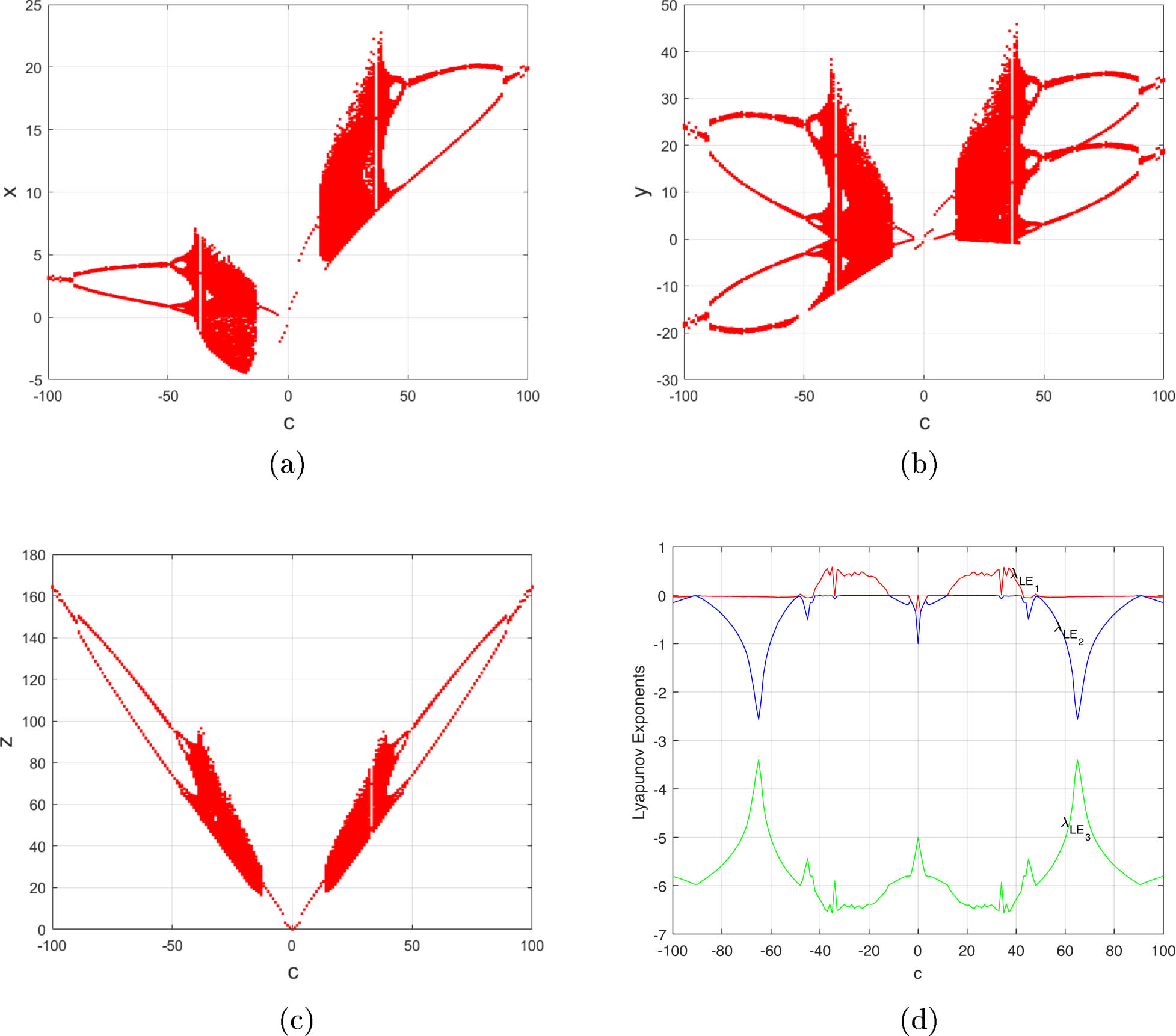
When

When
Third, set

When

When
Numerical Study 2.1 Set

For
Finally, using two appropriate Lyapunov functions and imitating the ones from previous literature [10–17, 29–38], we prove the following theorem in Section 3.
Theorem 2.2
If
In order to enhance the readability of the proof of the Section 3, the following symbols are introduced:
3 Heteroclinic orbit
In this section, we first give the following two Lyapunov functions and the corresponding derivatives along
(2)
Following the procedure in [10–17,29–39], one has to prove Lemma 3.1.
Lemma 3.1
Suppose
If
If
Proof
(i) Based on the hypothesis of (i) and Eqs (3.1) and (3.2), the fact
i.e.,
Since the boundedness of
(ii) First, we prove
Further, we prove that
Next the proof of Theorem 2.2 easily follows from Lemma 3.1.
Proof
(a) As
which suggests that
(b) Assume
i.e.
(c) In light of (a), one-dimensional branch of

When

When
4 Conclusion
In the sense of generalizing the second part of Hilbert’s renowned 16th problem, this study replaces the linear term
Compared with the controlled Lorenz, Chen, and Lü systems with various strange attractors (i.e., asymmetric two-wing ones, partial ones, and single-wing ones), the newly reported one only generates single-wing ones. To some extent, this exotic phenomenon contributes to the broader understanding of Hilbert’s sixteenth problem, i.e., the degree also makes a real impact on the geometrical structure of strange attractors, except for the number and mutual disposition [6,7,11–13].
However, it is unclear whether there are hidden single-wing Lorenz-like attractors in that studied system or not. In what follows, we will continue to uncover the correction between the degrees and strange attractors, and provide reference for real world applications. The asymmetric single-wing attractors proposed here have promising applications in secure communication, where their asymmetric dynamics can enhance signal encryption robustness against symmetric attacks. In neural networks, the single-wing structure could model asymmetric information processing in biological systems, such as directional signal transmission in neural circuits. For system identification, stitching the right and left images of single-wing Lorenz-like attractor with
-
Funding information: This work was supported in part by Zhejiang Public Welfare Technology Application Research Project of China under Grant LGN21F020003, and in part National Natural Science Foundation of China under Grant 12001489. Furthermore, the authors sincerely thank the anonymous editors and reviewers for their meticulous reading and constructive feedback, which have significantly enhanced the quality of this manuscript.
-
Author contributions: All authors have accepted responsibility for the entire content of this manuscript and approved its submission.
-
Conflict of interest: The authors state no conflict of interest.
-
Data availability statement: All data generated or analyzed during this study are included in this published article.
References
[1] Cox SM. The transition to chaos in an asymmetric perturbation of the Lorenz system. Phys Lett A. 1990;144(6–7):325–8. 10.1016/0375-9601(90)90134-ASearch in Google Scholar
[2] Lü J, Chen G, Zhang S. The compound structure of a new chaotic attractor. Chaos Solitons Fractals. 2002;14(5):669–72. 10.1016/S0960-0779(02)00007-3Search in Google Scholar
[3] Lü J, Zhou T, Chen G, Zhang S. The compound structure of Chen’s attractor. Int J Bifurcat Chaos. 2002;12(4):855–8. 10.1142/S0218127402004735Search in Google Scholar
[4] Liu J, Lu J, Wu X. Dynamical analysis for the compound structure of Chen’s system. ICARCV 2004 8th Control, Automation, Robotics and Vision Conference, Kunming, China. Vol. 3. 2004. p. 2250–3. 10.1109/ICARCV.2004.1469781Search in Google Scholar
[5] Miranda R, Stone E. The proto-Lorenz system. Phys Lett A. 1993;178:105–13. 10.1016/0375-9601(93)90735-ISearch in Google Scholar
[6] Leonov GA, Kuznetsov NV. On differences and similarities in the analysis of Lorenz, Chen, and Lu systems. Appl Math Comput. 2015;256:334–43. 10.1016/j.amc.2014.12.132Search in Google Scholar
[7] Kuznetsov NV, Mokaev TN, Kuznetsova OA, Kudryashova EV. The Lorenz system: hidden boundary of practical stability and the Lyapunov dimension. Nonlinear Dyn. 2020;102:713–32. 10.1007/s11071-020-05856-4Search in Google Scholar
[8] Hilbert D. Mathematical problems. Bull. Am. Math. Soc. 1902;8:437–79. 10.1090/S0002-9904-1902-00923-3Search in Google Scholar
[9] Zhang X, Chen G. Constructing an autonomous system with infinitely many chaotic attractors. Chaos Interdiscip J Nonlinear Sci. 2017;27(7):0711011–5. 10.1063/1.4986356Search in Google Scholar PubMed
[10] Liu Y, Yang Q. Dynamics of a new Lorenz-like chaotic system. Nonlinear Anal-Real. 2010;11(4):2563–72. 10.1016/j.nonrwa.2009.09.001Search in Google Scholar
[11] Wang H, Ke G, Pan J, Hu F, Fan H. Multitudinous potential hidden Lorenz-like attractors coined. Eur Phys J Spec Top. 2022;231:359–68. 10.1140/epjs/s11734-021-00423-3Search in Google Scholar
[12] Wang H, Pan J, Ke G. Revealing more hidden attractors from a new sub-quadratic Lorenz-like system of degree 65. Int J Bifurcat Chaos. 2024;34(6):2450071–15. 10.1142/S0218127424500718Search in Google Scholar
[13] Ke G, Pan J, Hu F, Wang H. Dynamics of a new four-thirds-degree sub-quadratic Lorenz-like system. Axioms. 2024;13(9):625–16. 10.3390/axioms13090625Search in Google Scholar
[14] Wang H, Ke G, Pan J, Su Q. Conjoined Lorenz-like attractors coined. Miskolc Mathematical Notes. 2023; code: MMN-4489, online, https://mat76.mat.uni-miskolc.hu/mnotes/forthcoming?volume=0&number=0#forthcoming. Search in Google Scholar
[15] Wang H, Pan J, Hu F, Ke G. Asymmetric singularly degenerate heteroclinic cycles. Int J Bifurcat Chaos. 2025;35(6):2550072-1–14. 10.1142/S0218127425500725Search in Google Scholar
[16] Li X, Wang H. A three-dimensional nonlinear system with a single heteroclinic trajectory. J Appl Anal Comput. 2020;10(1):249–66. 10.11948/20190135Search in Google Scholar
[17] Wang H, Pan J, Ke G, Hu F. A pair of centro-symmetric heteroclinic orbits coined. Adv Cont Discr Mod. 2024;2024:1–11. 10.1186/s13662-024-03809-4Search in Google Scholar
[18] Brunton SL, Proctor JL, Kutz JN. Discovering governing equations from data by sparse identification of nonlinear dynamical systems. PNAS. 2016;113(15):3932–7. 10.1073/pnas.1517384113Search in Google Scholar PubMed PubMed Central
[19] Wan Z, Sapsis TP. Reduced-space Gaussian process regression for data-driven probabilistic forecast of chaotic dynamical systems. Phys D. 2017;345(15):40–55. 10.1016/j.physd.2016.12.005Search in Google Scholar
[20] Dubois P, Gomez T, Planckaert L, Perret L. Data-driven predictions of the Lorenz system. Phys D. 2020;408:132495-1–10. 10.1016/j.physd.2020.132495Search in Google Scholar
[21] Karimov A, Rybin V, Kopets E, Karimov T, Nepomuceno E, Butusov D. Identifying empirical equations of chaotic circuit from data. Nonlinear Dyn. 2023;111:871–86. 10.1007/s11071-022-07854-0Search in Google Scholar
[22] Sprott JC. A proposed standard for the publication of new chaotic systems. Int J Bifurcat Chaos. 2011;21(9):2391–4. 10.1142/S021812741103009XSearch in Google Scholar
[23] Almutairi N, Saber S. Existence of chaos and the approximate solution of the Lorenz-Lü-Chen system with the Caputo fractional operator. AIP Advances. 2024;14:015112-1–16. 10.1063/5.0185906Search in Google Scholar
[24] Al-Raeei M, El-Daher MS. An algorithm for fractional Schrödinger equation in case of Morse potential. AIP Adv. 2020;10:035305-1–13. 10.1063/1.5113593Search in Google Scholar
[25] Tan H, Shi L, Wang S, Qu S. Improving model-free prediction of chaotic dynamics by purifying the incomplete input. AIP Adv. 2024;14:125225-1–10. 10.1063/5.0242605Search in Google Scholar
[26] Kuzenetsov YA. Elements of applied bifurcation theory. 3rd ed. New York: Springer-Verlag; 2004. Search in Google Scholar
[27] Sotomayor J, Mello LF, Braga DC. Lyapunov coefficients for degenerate Hopf bifurcations. arXiv:0709.3949v1 [Preprint]. 2007 [cited 2007 Sep 25]: [16 p.]. https://arxiv.org/abs/0709.3949. Search in Google Scholar
[28] Wolf A, Swift JB, Swinney HL, Vastano JA. Determining Lyapunov exponents from a time series. Phys D. 1985;16(3):285–317. 10.1016/0167-2789(85)90011-9Search in Google Scholar
[29] Tigan G, Constantinescu D. Heteroclinic orbits in the T and the Lü system. Chaos Solitons Fractals. 2009;42(1):20–3. 10.1016/j.chaos.2008.10.024Search in Google Scholar
[30] Chen Y, Yang Q. Dynamics of a hyperchaotic Lorenz-type system. Nonlinear Dyn. 2014;77(3):569–81. 10.1007/s11071-014-1318-0Search in Google Scholar
[31] Wang H, Li C, Li X. New heteroclinic orbits coined. Int J Bifurcat Chaos. 2016;26(12):16501941–13. 10.1142/S0218127416501947Search in Google Scholar
[32] Wang H, Ke G, Pan J, Hu F, Fan H, Su Q. Two pairs of heteroclinic orbits coined in a new sub-quadratic Lorenz-like system. Eur Phys J B. 2023;96:1–9. 10.1140/epjb/s10051-023-00491-5Search in Google Scholar
[33] Wang H, Ke G, Pan J, Su Q, Dong G, Fan H. Revealing the true and pseudo-singularly degenerate heteroclinic cycles. Indian J. Phys. 2023;976:3601–15. 10.1007/s12648-023-02689-wSearch in Google Scholar
[34] Wang H, Ke G, Pan J, Su Q. Modeling, dynamical analysis and numerical simulation of a new 3D cubic Lorenz-like system. Scientific Reports. 2023;13:6671–15. 10.1038/s41598-023-33826-4Search in Google Scholar PubMed PubMed Central
[35] Li Z, Ke G, Wang H, Pan J, Hu F, Su Q. Complex dynamics of a sub-quadratic Lorenz-like system. Open Phys. 2023;21:20220251-1–15. 10.1515/phys-2022-0251Search in Google Scholar
[36] Wang H, Ke G, Hu F, Pan J, Dong G, Chen G. Pseudo and true singularly degenerate heteroclinic cycles of a new 3D cubic Lorenz-like system. Results Phys. 2024;56:107243–13. 10.1016/j.rinp.2023.107243Search in Google Scholar
[37] Wang H, Pan J, Ke G. Multitudinous potential homoclinic and heteroclinic orbits seized. Electronic Res Archive. 2024;32(2):1003–16. 10.3934/era.2024049Search in Google Scholar
[38] Pan J, Wang H, Hu F. Revealing asymmetric homoclinic and heteroclinic orbits. Electronic Res Archive. 2025;33:1337–50. 10.3934/era.2025061Search in Google Scholar
[39] Pan J, Wang H, Hu F, Ke G. A novel Lorenz-like attractor and stability and equilibrium analysis. Axioms. 2025;14:264-1–17. 10.3390/axioms14040264Search in Google Scholar
© 2025 the author(s), published by De Gruyter
This work is licensed under the Creative Commons Attribution 4.0 International License.
Articles in the same Issue
- Research Articles
- Single-step fabrication of Ag2S/poly-2-mercaptoaniline nanoribbon photocathodes for green hydrogen generation from artificial and natural red-sea water
- Abundant new interaction solutions and nonlinear dynamics for the (3+1)-dimensional Hirota–Satsuma–Ito-like equation
- A novel gold and SiO2 material based planar 5-element high HPBW end-fire antenna array for 300 GHz applications
- Explicit exact solutions and bifurcation analysis for the mZK equation with truncated M-fractional derivatives utilizing two reliable methods
- Optical and laser damage resistance: Role of periodic cylindrical surfaces
- Numerical study of flow and heat transfer in the air-side metal foam partially filled channels of panel-type radiator under forced convection
- Water-based hybrid nanofluid flow containing CNT nanoparticles over an extending surface with velocity slips, thermal convective, and zero-mass flux conditions
- Dynamical wave structures for some diffusion--reaction equations with quadratic and quartic nonlinearities
- Solving an isotropic grey matter tumour model via a heat transfer equation
- Study on the penetration protection of a fiber-reinforced composite structure with CNTs/GFP clip STF/3DKevlar
- Influence of Hall current and acoustic pressure on nanostructured DPL thermoelastic plates under ramp heating in a double-temperature model
- Applications of the Belousov–Zhabotinsky reaction–diffusion system: Analytical and numerical approaches
- AC electroosmotic flow of Maxwell fluid in a pH-regulated parallel-plate silica nanochannel
- Interpreting optical effects with relativistic transformations adopting one-way synchronization to conserve simultaneity and space–time continuity
- Modeling and analysis of quantum communication channel in airborne platforms with boundary layer effects
- Theoretical and numerical investigation of a memristor system with a piecewise memductance under fractal–fractional derivatives
- Tuning the structure and electro-optical properties of α-Cr2O3 films by heat treatment/La doping for optoelectronic applications
- High-speed multi-spectral explosion temperature measurement using golden-section accelerated Pearson correlation algorithm
- Dynamic behavior and modulation instability of the generalized coupled fractional nonlinear Helmholtz equation with cubic–quintic term
- Study on the duration of laser-induced air plasma flash near thin film surface
- Exploring the dynamics of fractional-order nonlinear dispersive wave system through homotopy technique
- The mechanism of carbon monoxide fluorescence inside a femtosecond laser-induced plasma
- Numerical solution of a nonconstant coefficient advection diffusion equation in an irregular domain and analyses of numerical dispersion and dissipation
- Numerical examination of the chemically reactive MHD flow of hybrid nanofluids over a two-dimensional stretching surface with the Cattaneo–Christov model and slip conditions
- Impacts of sinusoidal heat flux and embraced heated rectangular cavity on natural convection within a square enclosure partially filled with porous medium and Casson-hybrid nanofluid
- Stability analysis of unsteady ternary nanofluid flow past a stretching/shrinking wedge
- Solitonic wave solutions of a Hamiltonian nonlinear atom chain model through the Hirota bilinear transformation method
- Bilinear form and soltion solutions for (3+1)-dimensional negative-order KdV-CBS equation
- Solitary chirp pulses and soliton control for variable coefficients cubic–quintic nonlinear Schrödinger equation in nonuniform management system
- Influence of decaying heat source and temperature-dependent thermal conductivity on photo-hydro-elasto semiconductor media
- Dissipative disorder optimization in the radiative thin film flow of partially ionized non-Newtonian hybrid nanofluid with second-order slip condition
- Bifurcation, chaotic behavior, and traveling wave solutions for the fractional (4+1)-dimensional Davey–Stewartson–Kadomtsev–Petviashvili model
- New investigation on soliton solutions of two nonlinear PDEs in mathematical physics with a dynamical property: Bifurcation analysis
- Mathematical analysis of nanoparticle type and volume fraction on heat transfer efficiency of nanofluids
- Creation of single-wing Lorenz-like attractors via a ten-ninths-degree term
- Optical soliton solutions, bifurcation analysis, chaotic behaviors of nonlinear Schrödinger equation and modulation instability in optical fiber
- Chaotic dynamics and some solutions for the (n + 1)-dimensional modified Zakharov–Kuznetsov equation in plasma physics
- Fractal formation and chaotic soliton phenomena in nonlinear conformable Heisenberg ferromagnetic spin chain equation
- Single-step fabrication of Mn(iv) oxide-Mn(ii) sulfide/poly-2-mercaptoaniline porous network nanocomposite for pseudo-supercapacitors and charge storage
- Novel constructed dynamical analytical solutions and conserved quantities of the new (2+1)-dimensional KdV model describing acoustic wave propagation
- Tavis–Cummings model in the presence of a deformed field and time-dependent coupling
- Spinning dynamics of stress-dependent viscosity of generalized Cross-nonlinear materials affected by gravitationally swirling disk
- Design and prediction of high optical density photovoltaic polymers using machine learning-DFT studies
- Robust control and preservation of quantum steering, nonlocality, and coherence in open atomic systems
- Coating thickness and process efficiency of reverse roll coating using a magnetized hybrid nanomaterial flow
- Dynamic analysis, circuit realization, and its synchronization of a new chaotic hyperjerk system
- Decoherence of steerability and coherence dynamics induced by nonlinear qubit–cavity interactions
- Finite element analysis of turbulent thermal enhancement in grooved channels with flat- and plus-shaped fins
- Modulational instability and associated ion-acoustic modulated envelope solitons in a quantum plasma having ion beams
- Statistical inference of constant-stress partially accelerated life tests under type II generalized hybrid censored data from Burr III distribution
- On solutions of the Dirac equation for 1D hydrogenic atoms or ions
- Entropy optimization for chemically reactive magnetized unsteady thin film hybrid nanofluid flow on inclined surface subject to nonlinear mixed convection and variable temperature
- Stability analysis, circuit simulation, and color image encryption of a novel four-dimensional hyperchaotic model with hidden and self-excited attractors
- A high-accuracy exponential time integration scheme for the Darcy–Forchheimer Williamson fluid flow with temperature-dependent conductivity
- Novel analysis of fractional regularized long-wave equation in plasma dynamics
- Development of a photoelectrode based on a bismuth(iii) oxyiodide/intercalated iodide-poly(1H-pyrrole) rough spherical nanocomposite for green hydrogen generation
- Investigation of solar radiation effects on the energy performance of the (Al2O3–CuO–Cu)/H2O ternary nanofluidic system through a convectively heated cylinder
- Quantum resources for a system of two atoms interacting with a deformed field in the presence of intensity-dependent coupling
- Studying bifurcations and chaotic dynamics in the generalized hyperelastic-rod wave equation through Hamiltonian mechanics
- A new numerical technique for the solution of time-fractional nonlinear Klein–Gordon equation involving Atangana–Baleanu derivative using cubic B-spline functions
- Interaction solutions of high-order breathers and lumps for a (3+1)-dimensional conformable fractional potential-YTSF-like model
- Hydraulic fracturing radioactive source tracing technology based on hydraulic fracturing tracing mechanics model
- Numerical solution and stability analysis of non-Newtonian hybrid nanofluid flow subject to exponential heat source/sink over a Riga sheet
- Numerical investigation of mixed convection and viscous dissipation in couple stress nanofluid flow: A merged Adomian decomposition method and Mohand transform
- Effectual quintic B-spline functions for solving the time fractional coupled Boussinesq–Burgers equation arising in shallow water waves
- Analysis of MHD hybrid nanofluid flow over cone and wedge with exponential and thermal heat source and activation energy
- Solitons and travelling waves structure for M-fractional Kairat-II equation using three explicit methods
- Impact of nanoparticle shapes on the heat transfer properties of Cu and CuO nanofluids flowing over a stretching surface with slip effects: A computational study
- Computational simulation of heat transfer and nanofluid flow for two-sided lid-driven square cavity under the influence of magnetic field
- Irreversibility analysis of a bioconvective two-phase nanofluid in a Maxwell (non-Newtonian) flow induced by a rotating disk with thermal radiation
- Hydrodynamic and sensitivity analysis of a polymeric calendering process for non-Newtonian fluids with temperature-dependent viscosity
- Exploring the peakon solitons molecules and solitary wave structure to the nonlinear damped Kortewege–de Vries equation through efficient technique
- Modeling and heat transfer analysis of magnetized hybrid micropolar blood-based nanofluid flow in Darcy–Forchheimer porous stenosis narrow arteries
- Activation energy and cross-diffusion effects on 3D rotating nanofluid flow in a Darcy–Forchheimer porous medium with radiation and convective heating
- Insights into chemical reactions occurring in generalized nanomaterials due to spinning surface with melting constraints
- Influence of a magnetic field on double-porosity photo-thermoelastic materials under Lord–Shulman theory
- Soliton-like solutions for a nonlinear doubly dispersive equation in an elastic Murnaghan's rod via Hirota's bilinear method
- Analytical and numerical investigation of exact wave patterns and chaotic dynamics in the extended improved Boussinesq equation
- Nonclassical correlation dynamics of Heisenberg XYZ states with (x, y)-spin--orbit interaction, x-magnetic field, and intrinsic decoherence effects
- Exact traveling wave and soliton solutions for chemotaxis model and (3+1)-dimensional Boiti–Leon–Manna–Pempinelli equation
- Unveiling the transformative role of samarium in ZnO: Exploring structural and optical modifications for advanced functional applications
- On the derivation of solitary wave solutions for the time-fractional Rosenau equation through two analytical techniques
- Analyzing the role of length and radius of MWCNTs in a nanofluid flow influenced by variable thermal conductivity and viscosity considering Marangoni convection
- Advanced mathematical analysis of heat and mass transfer in oscillatory micropolar bio-nanofluid flows via peristaltic waves and electroosmotic effects
- Exact bound state solutions of the radial Schrödinger equation for the Coulomb potential by conformable Nikiforov–Uvarov approach
- Some anisotropic and perfect fluid plane symmetric solutions of Einstein's field equations using killing symmetries
- Nonlinear dynamics of the dissipative ion-acoustic solitary waves in anisotropic rotating magnetoplasmas
- Curves in multiplicative equiaffine plane
- Exact solution of the three-dimensional (3D) Z2 lattice gauge theory
- Propagation properties of Airyprime pulses in relaxing nonlinear media
- Symbolic computation: Analytical solutions and dynamics of a shallow water wave equation in coastal engineering
- Wave propagation in nonlocal piezo-photo-hygrothermoelastic semiconductors subjected to heat and moisture flux
- Comparative reaction dynamics in rotating nanofluid systems: Quartic and cubic kinetics under MHD influence
- Laplace transform technique and probabilistic analysis-based hypothesis testing in medical and engineering applications
- Physical properties of ternary chloro-perovskites KTCl3 (T = Ge, Al) for optoelectronic applications
- Gravitational length stretching: Curvature-induced modulation of quantum probability densities
- The search for the cosmological cold dark matter axion – A new refined narrow mass window and detection scheme
- A comparative study of quantum resources in bipartite Lipkin–Meshkov–Glick model under DM interaction and Zeeman splitting
- PbO-doped K2O–BaO–Al2O3–B2O3–TeO2-glasses: Mechanical and shielding efficacy
- Nanospherical arsenic(iii) oxoiodide/iodide-intercalated poly(N-methylpyrrole) composite synthesis for broad-spectrum optical detection
- Sine power Burr X distribution with estimation and applications in physics and other fields
- Numerical modeling of enhanced reactive oxygen plasma in pulsed laser deposition of metal oxide thin films
- Dynamical analyses and dispersive soliton solutions to the nonlinear fractional model in stratified fluids
- Computation of exact analytical soliton solutions and their dynamics in advanced optical system
- An innovative approximation concerning the diffusion and electrical conductivity tensor at critical altitudes within the F-region of ionospheric plasma at low latitudes
- An analytical investigation to the (3+1)-dimensional Yu–Toda–Sassa–Fukuyama equation with dynamical analysis: Bifurcation
- Swirling-annular-flow-induced instability of a micro shell considering Knudsen number and viscosity effects
- Numerical analysis of non-similar convection flows of a two-phase nanofluid past a semi-infinite vertical plate with thermal radiation
- MgO NPs reinforced PCL/PVC nanocomposite films with enhanced UV shielding and thermal stability for packaging applications
- Optimal conditions for indoor air purification using non-thermal Corona discharge electrostatic precipitator
- Investigation of thermal conductivity and Raman spectra for HfAlB, TaAlB, and WAlB based on first-principles calculations
- Tunable double plasmon-induced transparency based on monolayer patterned graphene metamaterial
- DSC: depth data quality optimization framework for RGBD camouflaged object detection
- A new family of Poisson-exponential distributions with applications to cancer data and glass fiber reliability
- Numerical investigation of couple stress under slip conditions via modified Adomian decomposition method
- Monitoring plateau lake area changes in Yunnan province, southwestern China using medium-resolution remote sensing imagery: applicability of water indices and environmental dependencies
- Heterodyne interferometric fiber-optic gyroscope
- Exact solutions of Einstein’s field equations via homothetic symmetries of non-static plane symmetric spacetime
- A widespread study of discrete entropic model and its distribution along with fluctuations of energy
- Empirical model integration for accurate charge carrier mobility simulation in silicon MOSFETs
- The influence of scattering correction effect based on optical path distribution on CO2 retrieval
- Anisotropic dissociation and spectral response of 1-Bromo-4-chlorobenzene under static directional electric fields
- Role of tungsten oxide (WO3) on thermal and optical properties of smart polymer composites
- Analysis of iterative deblurring: no explicit noise
- The influence of anisotropy of InP on its elasticity and phonon properties
- Review Article
- Examination of the gamma radiation shielding properties of different clay and sand materials in the Adrar region
- Erratum
- Erratum to “On Soliton structures in optical fiber communications with Kundu–Mukherjee–Naskar model (Open Physics 2021;19:679–682)”
- Special Issue on Fundamental Physics from Atoms to Cosmos - Part II
- Possible explanation for the neutron lifetime puzzle
- Special Issue on Nanomaterial utilization and structural optimization - Part III
- Numerical investigation on fluid-thermal-electric performance of a thermoelectric-integrated helically coiled tube heat exchanger for coal mine air cooling
- Special Issue on Nonlinear Dynamics and Chaos in Physical Systems
- Analysis of the fractional relativistic isothermal gas sphere with application to neutron stars
- Abundant wave symmetries in the (3+1)-dimensional Chafee–Infante equation through the Hirota bilinear transformation technique
- Successive midpoint method for fractional differential equations with nonlocal kernels: Error analysis, stability, and applications
- Novel exact solitons to the fractional modified mixed-Korteweg--de Vries model with a stability analysis