Bifurcation, chaotic behavior, and traveling wave solutions for the fractional (4+1)-dimensional Davey–Stewartson–Kadomtsev–Petviashvili model
-
Zhao Li
 and
Yueyong Jiang
and
Yueyong Jiang

Abstract
This article investigates the traveling wave solution of the fractional (4+1)-dimensional Davey–Stewartson–Kadomtsev–Petviashvili model by using the complete discriminant system method. These solutions not only include rational function solutions, trigonometric function solutions, but also Jacobian function solutions. In order to illustrate the propagation of these solutions in the field of nonlinear optics and water wave models, some three-dimensional, two-dimensional, and contour maps are drawn. Meanwhile, the phase portrait of two-dimensional dynamical systems and its perturbation systems are studied using the planar dynamical system analysis method. By drawing phase diagrams, it is easy to observe the stability, periodicity, and chaotic behavior of two-dimensional dynamical systems through geometric visualization, which can also provide strong basis for researchers to design corresponding control systems.
1 Introduction
The fractional (4+1)-dimensional Davey–Stewartson–Kadomtsev–Petviashvili (DSKP) model is described as follows [1]:
where
The remaining sections are described as follows: in Section 2, the phase portraits and chaotic behaviors of two-dimensional dynamical system and its perturbation system are discussed. In Section 3, the solitary wave solutions of the fractional (4+1)-dimensional DSKP equation are constructed. In Section 4, three-dimensional, two-dimensional, and contour maps of some solutions of Eq. (1.1) are drawn. In Section 5, the solution obtained in this article is discussed in relation to existing solutions. In Section 6, a brief conclusion is given.
2 Bifurcation and chaotic behavior
Definition 2.1
[17] Let
where
Remark 2.2
In definition 2.1,
First, the wave transformation is given as follows:
where
Substituting Eq. (2.1) into Eq. (1.1) and integrating it twice, such that the first integration constant is zero and the second integration constant is non-zero, yields an ordinary differential equation
where
When
with Hamiltonian function
where
Here, we suppose that
If

2D phase portraits of Eq. (2.3). (a)
Next, we directly add a periodic disturbance to the second equation of system (2.3)
where
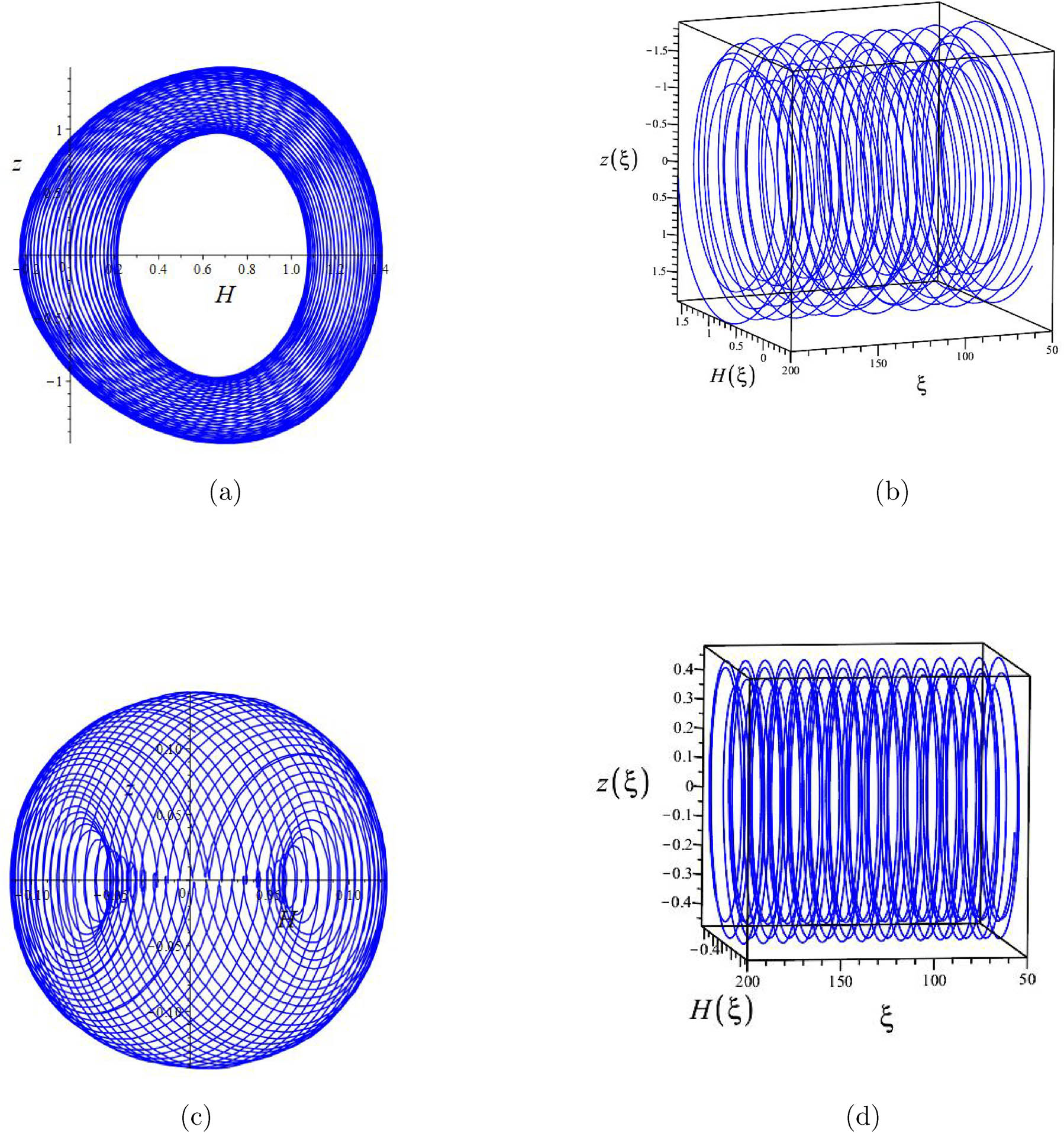
2D and 3D phase portraits of Eq. (2.3). (a)
3 Traveling wave solutions of Eq. (1.1)
According to the polynomial complete discriminant system method proposed by Professor Liu [22], we can obtain the single traveling wave solution of Eq. (1.1) in this section. In recent years, many experts [23–25] have utilized Professor Liu’s complete discriminant system method to construct single traveling wave solutions for nonlinear partial differential equations.
Multiplying both sides of Eq. (2.2) by
Here, we suppose that
Substituting Eq. (3.2) into Eq. (3.1), we have
here, let us assume that the third-order polynomial is
Therefore, the integral expression of Eq. (3.3) is
where
Case 1.
When
From Eqs (2.1) and (3.6), we obtain
Case 2.
Case 3.
When
where
When
Case 4.
When
4 Numerical simulation
In this section, we plotted the three-dimensional, two-dimensional, and contour plots of the two solutions
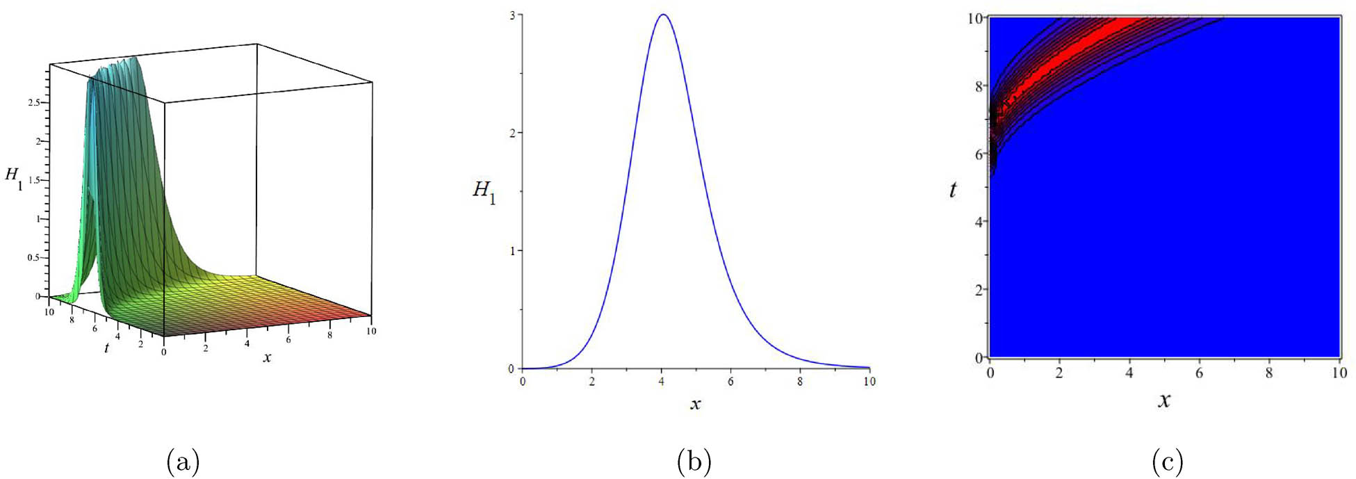
Graphics of
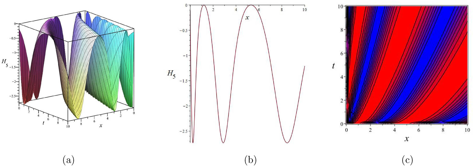
Graphics of
5 Discussion of results
Alsharidi et al. [1] obtained the exact solution of the DSKP equation using both the unified technique and modified extended tanh-expansion function technique, respectively. Compared with Alsharidi et al. [1], this article not only constructs the traveling wave solution of the DSKP equation using the fully discriminative system method, but also obtains the dynamic behavior of the DSKP equation using the planar dynamical system method. The solutions obtained in this article not only include common rational function solutions and trigonometric function solutions, but also more general Jacobian function solutions. In order to obtain the dynamic behavior of the equation more easily, this article also draws three-dimensional and two-dimensional phase diagrams of the two-dimensional dynamical system and its perturbation system. By analyzing the phase diagrams, it is easy to obtain the dynamic behavior of the two-dimensional dynamical system.
6 Conclusion
In this article, we obtained the traveling wave solution of the fractional (4+1)-dimensional DSKP equation. We not only discussed the planar phase portraits of the two-dimensional dynamical system of Eq. (1.1). Moreover, we have added periodic perturbations to the two-dimensional dynamical system and plotted the two-dimensional and three-dimensional phase prrtraits of the perturbed two-dimensional dynamical system. Based on Professor Liu’s complete discriminant system method, we obtained the Jacobian function solution, trigonometric function solution, and hyperbolic function solution of Eq. (1.1). We also simulated the obtained solutions by drawing three-dimensional, two-dimensional, and contour maps. In future work, we will continue to study soliton solutions of fractional-order partial differential equations, such as multi-soliton solutions or experimental validations.
-
Funding information: This research was supported by the Open Fund of Sichuan Provincial Key Laboratory of Ecological Security and Protection at Mianyang Normal University (Grant No. ESP2404).
-
Author contributions: Zhao Li: writing – orginal draft; Yueyong Jiang: supervision. All authors have accepted responsibility for the entire content of this manuscript and approved its submission.
-
Conflict of interest: The authors state no conflict of interest.
-
Data availability statement: Data sharing is not applicable to this article as no datasets were generated or analysed during the current study.
References
[1] Alsharidi AK, Junjua MUD. Kink, dark, bright, and singular optical solitons to the space-time nonlinear fractional (4+1)-dimensional Davey-Stewartson-Kadomtsev–Petviashvili model. Fractal Fract. 2024;8:388. 10.3390/fractalfract8070388Search in Google Scholar
[2] Ahmad I, Jalil A, Ullah A, Ahmad S, Sen MDI. Some new exact solutions of (4+1)-dimensional Davey-Stewartson-Kadomtsev–Petviashvili equation. Results Phys. 2023;45:106240. 10.1016/j.rinp.2023.106240Search in Google Scholar
[3] El-Shorbagy MA, Akram S, Rahman MU. Propagation of solitary wave solutions to (4+1)-dimensional Davey-Stewartson-Kadomtsev–Petviashvili equation arise in mathematical physics and stability analysis. Partial Differ Eq Appl Math. 2024;10:100669. 10.1016/j.padiff.2024.100669Search in Google Scholar
[4] Ahmad S, Ullah A, Ahmad S, Saifullah S, Shokri A. Periodic solitons of Davey Stewartson Kadomtsev Petviashvili equation in (4+1)-dimension. Results Phys. 2023;50:106547. 10.1016/j.rinp.2023.106547Search in Google Scholar
[5] Rehman HU, Said GS, Amer A, Ashraf H, Tharwa MMt, Abdel-Aty M, et al. Unraveling the (4+1)-dimensional Davey-Stewartson-Kadomtsev–Petviashvili equation:Exploring soliton solutions via multiple techniques. Alex Eng J. 2024;90:17–23. 10.1016/j.aej.2024.01.058Search in Google Scholar
[6] Rabie WB, Khalil TA, Badra N, Ahmed HM, Mirzazadeh M, Hashemi MS. Soliton solutions and other solutions to the (4+1)-dimensional Davey-Stewartson-Kadomtsev–Petviashvili equation using modified extended mapping method. Qual Theor of Dyn Syst. 2024;23:87. 10.1007/s12346-023-00944-3Search in Google Scholar
[7] Li CY. Zero-r Law on the analyticity and the uniform continuity of fractional resolvent families. Integr Equat Oper Th. 2024;96:34. 10.1007/s00020-024-02785-4Search in Google Scholar
[8] Li CY. The Hautus-type inequality for abstract fractional Cauchy problems and its observability. J Math. 2024;2024:6179980. 10.1155/2024/6179980Search in Google Scholar
[9] Zhao S, Li Z. The analysis of traveling wave solutions and dynamical behavior for the stochastic coupled Maccarias system via Brownian motion. Ain Shams Eng J. 2024;15:103037. 10.1016/j.asej.2024.103037Search in Google Scholar
[10] He YL, Kai Y. Wave structures, modulation instability analysis and chaotic behaviors to Kudryashovas equation with third-order dispersion. Nonlinear Dynam. 2024;112:10355–71. 10.1007/s11071-024-09635-3Search in Google Scholar
[11] Zhu CY, Idris SA, Abdalla MEM, Rezapour S, Shateyi S, Gunay B. Analytical study of nonlinear models using a modified Schrödingeras equation and logarithmic transformation. Results Phys. 2023;55:107183. 10.1016/j.rinp.2023.107183Search in Google Scholar
[12] Seadawy AR, Arshad M, Lu DC. The weakly nonlinear wave propagation theory for the Kelvin-Helmholtz instability in magnetohydrodynamics flows. Chaos Soliton Fract. 2020;139:110141. 10.1016/j.chaos.2020.110141Search in Google Scholar
[13] Chen D, Shi D, Chen F. Qualitative analysis and new traveling wave solutions for the stochastic Biswas-Milovic equation. AIMS Math. 2025;10:4092–7. 10.3934/math.2025190Search in Google Scholar
[14] Zhang K, Cao JP, Lyu JJ. Dynamic behavior and modulation instability for a generalized nonlinear Schrödinger equation with nonlocal nonlinearity. Phys Scripta. 2024;100:015262. Search in Google Scholar
[15] Zhao S. Chaos analysis and traveling wave solutions for fractional (3+1)-dimensional Wazwaz Kaur Boussinesq equation with beta derivative. Sci Rep-UK. 2024;14:23034. 10.1038/s41598-024-74606-ySearch in Google Scholar PubMed PubMed Central
[16] Liu CY. The traveling wave solution and dynamics analysis of the fractional-order generalized Pochhammer-Chree equation. AIMS Math. 2024;9:33956–16. 10.3934/math.20241619Search in Google Scholar
[17] Luo J, Li Z. Dynamic behavior and optical soliton for the M-Truncated fractional Paraxial wave equation arising in a liquid crystal model. Fractal Fract. 2024;8:348. 10.3390/fractalfract8060348Search in Google Scholar
[18] Farooq A, Khan MI, Nisar KS, Shah NA. A detailed analysis of the improved modified Korteweg-de Vries equation via the Jacobi elliptic function expansion method and the application of truncated M-fractional derivatives. Results Phys. 2024;59:107604. 10.1016/j.rinp.2024.107604Search in Google Scholar
[19] Li Z, Lyu JJ, Hussain E. Bifurcation, chaotic behaviors and solitary wave solutions for the fractional Twin-Core couplers with Kerr law non-linearity. Sci Rep-UK. 2024;14:22616. 10.1038/s41598-024-74044-wSearch in Google Scholar PubMed PubMed Central
[20] Zhang K, Cao JP, Lyu JJ. Dynamic behavior and modulation instability for a generalized nonlinear Schrödinger equation with nonlocal nonlinearity. Phys Scripta. 2025;100:015262. 10.1088/1402-4896/ad9cfaSearch in Google Scholar
[21] Li Z, Zhao S. Bifurcation, chaotic behavior and solitary wave solutions for the Akbota equation. AIMS Math. 2024;9:22590–11. 10.3934/math.20241100Search in Google Scholar
[22] Liu CS. Applications of complete discrimination system for polynomial for classifications of traveling wave solutions to nonlinear differential equations. Comput Phys Commun. 2010;181:317–7. 10.1016/j.cpc.2009.10.006Search in Google Scholar
[23] Gu MS, Li JL, Liu FM, Li Z, Peng C. Propagation of traveling wave solution of the strain wave equation in microcrystalline materials. Open Phys. 2024;22:20240093. 10.1515/phys-2024-0093Search in Google Scholar
[24] Liu CY. The chaotic behavior and traveling wave solutions of the conformable extended Korteweg-de-Vries model. Open Phys. 2024;22:20240069. 10.1515/phys-2024-0069Search in Google Scholar
[25] Gu MS, Liu FM, Li JL, Peng C, Li Z. Explicit solutions of the generalized Kudryashovas equation with truncated M-fractional derivative. Sci Rep-UK. 2024;14:21714. 10.1038/s41598-024-72610-wSearch in Google Scholar PubMed PubMed Central
© 2025 the author(s), published by De Gruyter
This work is licensed under the Creative Commons Attribution 4.0 International License.
Articles in the same Issue
- Research Articles
- Single-step fabrication of Ag2S/poly-2-mercaptoaniline nanoribbon photocathodes for green hydrogen generation from artificial and natural red-sea water
- Abundant new interaction solutions and nonlinear dynamics for the (3+1)-dimensional Hirota–Satsuma–Ito-like equation
- A novel gold and SiO2 material based planar 5-element high HPBW end-fire antenna array for 300 GHz applications
- Explicit exact solutions and bifurcation analysis for the mZK equation with truncated M-fractional derivatives utilizing two reliable methods
- Optical and laser damage resistance: Role of periodic cylindrical surfaces
- Numerical study of flow and heat transfer in the air-side metal foam partially filled channels of panel-type radiator under forced convection
- Water-based hybrid nanofluid flow containing CNT nanoparticles over an extending surface with velocity slips, thermal convective, and zero-mass flux conditions
- Dynamical wave structures for some diffusion--reaction equations with quadratic and quartic nonlinearities
- Solving an isotropic grey matter tumour model via a heat transfer equation
- Study on the penetration protection of a fiber-reinforced composite structure with CNTs/GFP clip STF/3DKevlar
- Influence of Hall current and acoustic pressure on nanostructured DPL thermoelastic plates under ramp heating in a double-temperature model
- Applications of the Belousov–Zhabotinsky reaction–diffusion system: Analytical and numerical approaches
- AC electroosmotic flow of Maxwell fluid in a pH-regulated parallel-plate silica nanochannel
- Interpreting optical effects with relativistic transformations adopting one-way synchronization to conserve simultaneity and space–time continuity
- Modeling and analysis of quantum communication channel in airborne platforms with boundary layer effects
- Theoretical and numerical investigation of a memristor system with a piecewise memductance under fractal–fractional derivatives
- Tuning the structure and electro-optical properties of α-Cr2O3 films by heat treatment/La doping for optoelectronic applications
- High-speed multi-spectral explosion temperature measurement using golden-section accelerated Pearson correlation algorithm
- Dynamic behavior and modulation instability of the generalized coupled fractional nonlinear Helmholtz equation with cubic–quintic term
- Study on the duration of laser-induced air plasma flash near thin film surface
- Exploring the dynamics of fractional-order nonlinear dispersive wave system through homotopy technique
- The mechanism of carbon monoxide fluorescence inside a femtosecond laser-induced plasma
- Numerical solution of a nonconstant coefficient advection diffusion equation in an irregular domain and analyses of numerical dispersion and dissipation
- Numerical examination of the chemically reactive MHD flow of hybrid nanofluids over a two-dimensional stretching surface with the Cattaneo–Christov model and slip conditions
- Impacts of sinusoidal heat flux and embraced heated rectangular cavity on natural convection within a square enclosure partially filled with porous medium and Casson-hybrid nanofluid
- Stability analysis of unsteady ternary nanofluid flow past a stretching/shrinking wedge
- Solitonic wave solutions of a Hamiltonian nonlinear atom chain model through the Hirota bilinear transformation method
- Bilinear form and soltion solutions for (3+1)-dimensional negative-order KdV-CBS equation
- Solitary chirp pulses and soliton control for variable coefficients cubic–quintic nonlinear Schrödinger equation in nonuniform management system
- Influence of decaying heat source and temperature-dependent thermal conductivity on photo-hydro-elasto semiconductor media
- Dissipative disorder optimization in the radiative thin film flow of partially ionized non-Newtonian hybrid nanofluid with second-order slip condition
- Bifurcation, chaotic behavior, and traveling wave solutions for the fractional (4+1)-dimensional Davey–Stewartson–Kadomtsev–Petviashvili model
- New investigation on soliton solutions of two nonlinear PDEs in mathematical physics with a dynamical property: Bifurcation analysis
- Mathematical analysis of nanoparticle type and volume fraction on heat transfer efficiency of nanofluids
- Creation of single-wing Lorenz-like attractors via a ten-ninths-degree term
- Optical soliton solutions, bifurcation analysis, chaotic behaviors of nonlinear Schrödinger equation and modulation instability in optical fiber
- Chaotic dynamics and some solutions for the (n + 1)-dimensional modified Zakharov–Kuznetsov equation in plasma physics
- Fractal formation and chaotic soliton phenomena in nonlinear conformable Heisenberg ferromagnetic spin chain equation
- Single-step fabrication of Mn(iv) oxide-Mn(ii) sulfide/poly-2-mercaptoaniline porous network nanocomposite for pseudo-supercapacitors and charge storage
- Novel constructed dynamical analytical solutions and conserved quantities of the new (2+1)-dimensional KdV model describing acoustic wave propagation
- Tavis–Cummings model in the presence of a deformed field and time-dependent coupling
- Spinning dynamics of stress-dependent viscosity of generalized Cross-nonlinear materials affected by gravitationally swirling disk
- Design and prediction of high optical density photovoltaic polymers using machine learning-DFT studies
- Robust control and preservation of quantum steering, nonlocality, and coherence in open atomic systems
- Coating thickness and process efficiency of reverse roll coating using a magnetized hybrid nanomaterial flow
- Dynamic analysis, circuit realization, and its synchronization of a new chaotic hyperjerk system
- Decoherence of steerability and coherence dynamics induced by nonlinear qubit–cavity interactions
- Finite element analysis of turbulent thermal enhancement in grooved channels with flat- and plus-shaped fins
- Modulational instability and associated ion-acoustic modulated envelope solitons in a quantum plasma having ion beams
- Statistical inference of constant-stress partially accelerated life tests under type II generalized hybrid censored data from Burr III distribution
- On solutions of the Dirac equation for 1D hydrogenic atoms or ions
- Entropy optimization for chemically reactive magnetized unsteady thin film hybrid nanofluid flow on inclined surface subject to nonlinear mixed convection and variable temperature
- Stability analysis, circuit simulation, and color image encryption of a novel four-dimensional hyperchaotic model with hidden and self-excited attractors
- A high-accuracy exponential time integration scheme for the Darcy–Forchheimer Williamson fluid flow with temperature-dependent conductivity
- Novel analysis of fractional regularized long-wave equation in plasma dynamics
- Development of a photoelectrode based on a bismuth(iii) oxyiodide/intercalated iodide-poly(1H-pyrrole) rough spherical nanocomposite for green hydrogen generation
- Investigation of solar radiation effects on the energy performance of the (Al2O3–CuO–Cu)/H2O ternary nanofluidic system through a convectively heated cylinder
- Quantum resources for a system of two atoms interacting with a deformed field in the presence of intensity-dependent coupling
- Studying bifurcations and chaotic dynamics in the generalized hyperelastic-rod wave equation through Hamiltonian mechanics
- A new numerical technique for the solution of time-fractional nonlinear Klein–Gordon equation involving Atangana–Baleanu derivative using cubic B-spline functions
- Interaction solutions of high-order breathers and lumps for a (3+1)-dimensional conformable fractional potential-YTSF-like model
- Hydraulic fracturing radioactive source tracing technology based on hydraulic fracturing tracing mechanics model
- Numerical solution and stability analysis of non-Newtonian hybrid nanofluid flow subject to exponential heat source/sink over a Riga sheet
- Numerical investigation of mixed convection and viscous dissipation in couple stress nanofluid flow: A merged Adomian decomposition method and Mohand transform
- Effectual quintic B-spline functions for solving the time fractional coupled Boussinesq–Burgers equation arising in shallow water waves
- Analysis of MHD hybrid nanofluid flow over cone and wedge with exponential and thermal heat source and activation energy
- Solitons and travelling waves structure for M-fractional Kairat-II equation using three explicit methods
- Impact of nanoparticle shapes on the heat transfer properties of Cu and CuO nanofluids flowing over a stretching surface with slip effects: A computational study
- Computational simulation of heat transfer and nanofluid flow for two-sided lid-driven square cavity under the influence of magnetic field
- Irreversibility analysis of a bioconvective two-phase nanofluid in a Maxwell (non-Newtonian) flow induced by a rotating disk with thermal radiation
- Hydrodynamic and sensitivity analysis of a polymeric calendering process for non-Newtonian fluids with temperature-dependent viscosity
- Exploring the peakon solitons molecules and solitary wave structure to the nonlinear damped Kortewege–de Vries equation through efficient technique
- Modeling and heat transfer analysis of magnetized hybrid micropolar blood-based nanofluid flow in Darcy–Forchheimer porous stenosis narrow arteries
- Activation energy and cross-diffusion effects on 3D rotating nanofluid flow in a Darcy–Forchheimer porous medium with radiation and convective heating
- Insights into chemical reactions occurring in generalized nanomaterials due to spinning surface with melting constraints
- Influence of a magnetic field on double-porosity photo-thermoelastic materials under Lord–Shulman theory
- Soliton-like solutions for a nonlinear doubly dispersive equation in an elastic Murnaghan's rod via Hirota's bilinear method
- Analytical and numerical investigation of exact wave patterns and chaotic dynamics in the extended improved Boussinesq equation
- Nonclassical correlation dynamics of Heisenberg XYZ states with (x, y)-spin--orbit interaction, x-magnetic field, and intrinsic decoherence effects
- Exact traveling wave and soliton solutions for chemotaxis model and (3+1)-dimensional Boiti–Leon–Manna–Pempinelli equation
- Unveiling the transformative role of samarium in ZnO: Exploring structural and optical modifications for advanced functional applications
- On the derivation of solitary wave solutions for the time-fractional Rosenau equation through two analytical techniques
- Analyzing the role of length and radius of MWCNTs in a nanofluid flow influenced by variable thermal conductivity and viscosity considering Marangoni convection
- Advanced mathematical analysis of heat and mass transfer in oscillatory micropolar bio-nanofluid flows via peristaltic waves and electroosmotic effects
- Exact bound state solutions of the radial Schrödinger equation for the Coulomb potential by conformable Nikiforov–Uvarov approach
- Some anisotropic and perfect fluid plane symmetric solutions of Einstein's field equations using killing symmetries
- Nonlinear dynamics of the dissipative ion-acoustic solitary waves in anisotropic rotating magnetoplasmas
- Curves in multiplicative equiaffine plane
- Exact solution of the three-dimensional (3D) Z2 lattice gauge theory
- Propagation properties of Airyprime pulses in relaxing nonlinear media
- Symbolic computation: Analytical solutions and dynamics of a shallow water wave equation in coastal engineering
- Wave propagation in nonlocal piezo-photo-hygrothermoelastic semiconductors subjected to heat and moisture flux
- Comparative reaction dynamics in rotating nanofluid systems: Quartic and cubic kinetics under MHD influence
- Laplace transform technique and probabilistic analysis-based hypothesis testing in medical and engineering applications
- Physical properties of ternary chloro-perovskites KTCl3 (T = Ge, Al) for optoelectronic applications
- Gravitational length stretching: Curvature-induced modulation of quantum probability densities
- The search for the cosmological cold dark matter axion – A new refined narrow mass window and detection scheme
- A comparative study of quantum resources in bipartite Lipkin–Meshkov–Glick model under DM interaction and Zeeman splitting
- PbO-doped K2O–BaO–Al2O3–B2O3–TeO2-glasses: Mechanical and shielding efficacy
- Nanospherical arsenic(iii) oxoiodide/iodide-intercalated poly(N-methylpyrrole) composite synthesis for broad-spectrum optical detection
- Sine power Burr X distribution with estimation and applications in physics and other fields
- Numerical modeling of enhanced reactive oxygen plasma in pulsed laser deposition of metal oxide thin films
- Dynamical analyses and dispersive soliton solutions to the nonlinear fractional model in stratified fluids
- Computation of exact analytical soliton solutions and their dynamics in advanced optical system
- An innovative approximation concerning the diffusion and electrical conductivity tensor at critical altitudes within the F-region of ionospheric plasma at low latitudes
- An analytical investigation to the (3+1)-dimensional Yu–Toda–Sassa–Fukuyama equation with dynamical analysis: Bifurcation
- Swirling-annular-flow-induced instability of a micro shell considering Knudsen number and viscosity effects
- Numerical analysis of non-similar convection flows of a two-phase nanofluid past a semi-infinite vertical plate with thermal radiation
- MgO NPs reinforced PCL/PVC nanocomposite films with enhanced UV shielding and thermal stability for packaging applications
- Optimal conditions for indoor air purification using non-thermal Corona discharge electrostatic precipitator
- Investigation of thermal conductivity and Raman spectra for HfAlB, TaAlB, and WAlB based on first-principles calculations
- Tunable double plasmon-induced transparency based on monolayer patterned graphene metamaterial
- DSC: depth data quality optimization framework for RGBD camouflaged object detection
- A new family of Poisson-exponential distributions with applications to cancer data and glass fiber reliability
- Numerical investigation of couple stress under slip conditions via modified Adomian decomposition method
- Monitoring plateau lake area changes in Yunnan province, southwestern China using medium-resolution remote sensing imagery: applicability of water indices and environmental dependencies
- Heterodyne interferometric fiber-optic gyroscope
- Exact solutions of Einstein’s field equations via homothetic symmetries of non-static plane symmetric spacetime
- A widespread study of discrete entropic model and its distribution along with fluctuations of energy
- Empirical model integration for accurate charge carrier mobility simulation in silicon MOSFETs
- The influence of scattering correction effect based on optical path distribution on CO2 retrieval
- Anisotropic dissociation and spectral response of 1-Bromo-4-chlorobenzene under static directional electric fields
- Role of tungsten oxide (WO3) on thermal and optical properties of smart polymer composites
- Analysis of iterative deblurring: no explicit noise
- The influence of anisotropy of InP on its elasticity and phonon properties
- Review Article
- Examination of the gamma radiation shielding properties of different clay and sand materials in the Adrar region
- Erratum
- Erratum to “On Soliton structures in optical fiber communications with Kundu–Mukherjee–Naskar model (Open Physics 2021;19:679–682)”
- Special Issue on Fundamental Physics from Atoms to Cosmos - Part II
- Possible explanation for the neutron lifetime puzzle
- Special Issue on Nanomaterial utilization and structural optimization - Part III
- Numerical investigation on fluid-thermal-electric performance of a thermoelectric-integrated helically coiled tube heat exchanger for coal mine air cooling
- Special Issue on Nonlinear Dynamics and Chaos in Physical Systems
- Analysis of the fractional relativistic isothermal gas sphere with application to neutron stars
- Abundant wave symmetries in the (3+1)-dimensional Chafee–Infante equation through the Hirota bilinear transformation technique
- Successive midpoint method for fractional differential equations with nonlocal kernels: Error analysis, stability, and applications
- Novel exact solitons to the fractional modified mixed-Korteweg--de Vries model with a stability analysis