Influence of a magnetic field on double-porosity photo-thermoelastic materials under Lord–Shulman theory
-
Khaled Lotfy

 ,
Ibrahim S. Elshazly
,
Ibrahim S. Elshazly

Abstract
This study explores the influence of a magnetic field on a two-dimensional photo-thermoelastic material with a dual porous structure, based on the Lord–Shulman theory of thermoelasticity. The model presents a novel approach to understanding magneto-thermoelastic interactions in such elastic semiconductor materials. The model incorporates the Lorentz force to account for magnetoelastic interactions and considers a uniform double-porosity thermoelastic half-space. Analytical expressions for key physical quantities are derived using the normal mode analysis technique, assuming exponential representations for the variables. The governing equations for the generalized double-porosity structure of photo-thermoelastic materials, incorporating a single relaxation time, are formulated and solved under specific boundary conditions. The results provide insights into the coupled behavior of thermal, elastic, and electromagnetic fields in dual-porosity materials and highlight the significant role of magnetic fields in influencing wave propagation and stress distribution. The work underscores the critical role of magnetic fields in altering wave propagation and stress behavior, offering potential advancements in materials science and engineering applications.
Nomenclature
-
-
Lame’ parameters (Pa (N/m2)
-
-
displacement vector (m)
-
-
Kronecker delta
-
-
mass density (kg/m3)
-
-
relaxation time (s)
-
-
photogenerated carrier lifetime (s)
-
-
the energy gap of the semiconductor (eV)
-
-
specific heat at constant strain (J/(kg K))
-
-
carrier diffusion coefficient (m2/s)
-
-
carrier concentration at temperature
-
-
stress tensor (Pa (N/m2))
-
-
volume fraction field corresponding to pores
-
-
volume fraction field corresponding to fissures
-
-
volume fraction fields corresponding to
-
-
volume coefficient of thermal expansion (W/(m K))
-
-
thermal conductivity (K−1)
-
-
acoefficients of equilibrated inertia (kg/m3)
-
-
reference temperature (K)
-
-
constitutive coefficients (Pa (N/m2))
-
-
equilibrated stress corresponding to
-
-
equilibrated stress corresponding to
-
-
temperature change measured at
-
-
thermoelastic coupling parameter
-
-
thermoenergy coupling parameter
-
-
thermoelectric coupling parameter
1 Introduction
The study of the influence of magnetic fields on two-dimensional photo-thermoelastic materials with a dual porous structure has significant implications for real-world applications. Such materials are integral in advanced engineering and technology fields, including aerospace, biomedical devices, and geophysical exploration. Understanding their behavior under magnetic and thermal effects enables the development of sensors and actuators that operate reliably in harsh environments. For example, these materials can be used in magnetic field sensors for medical imaging or as components in devices requiring precise thermal and mechanical stability, such as energy storage systems and structural health monitoring. Moreover, the incorporation of dual porosity in the analysis allows for better modeling of materials like rocks or porous composites, which are crucial in oil extraction, carbon sequestration, and earthquake prediction. By combining theoretical advancements like the Lord–Shulman (L-S) theory and practical considerations, this study paves the way for innovations in material design and multifunctional device applications.
Photo-thermoelasticity is the study of the coupled behavior of thermal, elastic, and optical properties in materials under stress [1]. This field is particularly relevant in the analysis of complex materials, such as porous media, which exhibit intricate behaviors due to their internal structure. Double porosity [2,3,4] describes a material possessing two distinct pore systems, leading to complex mechanical and thermal responses. The study focuses on the interaction between light and materials subjected to thermal stress, which allows for the measurement of stress and strain using optical techniques, specifically photoelasticity. The governing equations of photo-thermoelasticity incorporate the principles of thermodynamics, elasticity, and optics. Double-porosity models are employed to characterize materials with two separate pore networks, a concept that is particularly important for materials such as rocks, soils, and certain biological tissues [5]. The two-pore systems can interact, influencing the material’s overall mechanical and thermal properties. The thermal behavior in double-porosity media is complex, as the heat transport mechanisms in each pore network differ. Consequently, thermal expansion and conduction may vary significantly between the two systems, leading to heterogeneous stress distributions. The L-S theory of thermoelasticity, introduced in 1967, incorporates a single relaxation time for the thermoelastic process, accounting for the time-dependent response of the material [6].
Double porosity refers to a material with two distinct pore systems: macropores and larger pores that dominate the bulk material, and microfissures indicate smaller cracks or fissures within the material. The interaction between these two pore systems influences the material’s thermal and mechanical properties, making it suitable for applications such as oil and gas extraction and geothermal energy systems. The linear theory of elastic materials with double porosity was first introduced in the publications by Barenblatt et al. [7,8]. Khalili and Valliappan [9] utilized the idea of flow and deformation in double-porous media. Masters et al. conducted a study on the correlation between temperature and a twofold porosity model of deformable porous media [10]. Khalili and Selvadurai [11] examined the comprehensive coupled constitutive model for thermo-hydro-mechanical analysis in elastic media with dual porosity. Zhao and Chen [12] presented a comprehensive dual-porosity model that is fully coupled and applicable to anisotropic formations. Svanadze [13] investigated the dynamic issues related to the theory of elasticity in solids with dual porosity. Ainouz researched the homogenized double-porosity models for poro-elastic media featuring an interfacial flow barrier [14]. Svanadze [15] conducted research on the theory of elasticity for solids with double porosity, specifically focusing on plane waves and boundary value problems. In their study, Straughan [16] examined the stability and uniqueness of elasticity in a double-porosity system.
Previously, academics have explored many issues related to magnetic fields. Mahato and Biswas [17] specifically examined the state space method, three-phase-lag model, Rayleigh waves, Eringen’s nonlocal thermoelasticity, and double porosity. Berryman and Wang [18] have devised analytical and numerical techniques to solve the intricate equations that govern thermoelasticity in materials with dual porosity. Finite element analysis and boundary element techniques are frequently employed to model the response of these materials under different thermal and mechanical loads [3]. Experimental studies are essential for verifying theoretical models of thermoelasticity in double-porosity materials. Thermal loading experiments, acoustic emission monitoring, and digital image correlation techniques are used to quantify the stress and strain responses of materials having double porosity under controlled settings. The investigation of thermoelasticity in double-porosity materials holds great importance in various domains like geothermal energy extraction, petroleum engineering, and materials science. Gaining insight into the thermal and mechanical characteristics of rocks with dual porosity is crucial for maximizing the efficiency of resource extraction from underground formations. Furthermore, researchers [19] are currently investigating synthetic materials that include customized double-porosity architectures for applications in enhanced insulation, filtration, and medicinal implants.
An essential obstacle in this domain is the intricacy of the models needed to precisely depict the behavior of double-porosity materials when subjected to thermoelastic loading. These models typically necessitate advanced numerical techniques for their resolution, which can be computationally demanding. Another difficulty lies in the integration of multiple physical processes, such as heat transport, fluid flow, and mechanical deformation, into a cohesive model. Subsequent studies could prioritize the development of more streamlined algorithms and computational strategies to manage these interconnected activities. Precisely determining the material parameters of double-porosity systems, including permeability, thermal conductivity, and elastic moduli, is crucial for enhancing the accuracy of predictive models. Progress in imaging techniques and material testing will be pivotal in this field. Double porosity models are employed to characterize materials that possess two distinct pore networks. This concept is especially significant in the examination of materials such as rocks, dirt, and certain biological tissues. Interactions between the two pore systems can have an impact on the material’s overall mechanical and thermal properties. The thermal effects in porous media with double porosity are intricate because of the distinct heat transport mechanisms in the two-pore networks. The thermal expansion and conduction in the two systems might vary greatly, resulting in distinct stress distributions.
Marin and Marinescu [20] further examine dipolar thermoelastic materials, a particular case of multipolar continuum mechanics. This hypothesis posits the existence of two porosity types: macroporosity, denoting the presence of pores inside the material, and microporosity, indicating the presence of minute fissures within the porous structure. The theory of thermoelastic dynamics is analyzed for materials with a dual-porosity structure and microtemperature. This study is distinctive as it addresses an issue of double-porous thermoelastic materials with microtemperature, previously examined by Florea [21]. The originality resides in the exploration of a temporal regression problem. The research examines Rayleigh-type waves in a layered model comprising a thermoelastic material with a dual porosity structure. The dispersion relation is obtained by implementing appropriate boundary conditions, demonstrating the existence of multiple modes and the dispersive and attenuative properties of Rayleigh-type waves. The dispersion relation reduces to the dispersion equation for Stoneley-type waves when Kumar et al. [22] posit that the thickness of the overlying layer is sufficiently substantial. Arusoaie [23] examines the spatial and temporal properties of solutions to the initial boundary value problem associated with the linear theory of thermoelastic materials exhibiting a double porosity structure. We examine two appropriate time-weighted integral measures and develop exponential estimates that define the spatial characteristics of solutions. Rana et al. [24] performed a study on the vibrational characteristics of a hollow cylinder composed of a homogeneous and isotropic elastic material exhibiting double porosity. The study focuses on the impact of a magnetic field on the cylinder’s behavior, particularly with nonlocal elasticity. Kumar and Vohra [25] investigated the vibration behavior of a microbeam with a twofold porosity structure (TDP), which is both homogenous and isotropic. This vibration is caused by pulsed laser heating. The study is conducted within the L-S’s theory of thermoelasticity, which includes one relaxation time. Seema and Singhal [26,27] explored how wave propagation affects SAW macro- and nanosensors. Thus, shear horizontal (SH) waves are studied in an orthotropic piezoelectric quasicrystal (PQC) layer above an elastic framework (Model I), a piezoelectric substrate, and an orthotropic PQC substrate (Model II) using surface piezoelectricity theory. Previous research on surface acoustic wave sensors found significant restrictions in piezoelectric material selection and wave propagation orientation [28]. They study how wave propagation direction affects SAW macro and nanosensor efficacy to overcome technical barriers. A model is proposed to examine SH and anti-plane SH wave propagation in piezoelectric materials, considering surface effects. Seema and Singhal [26,29] discussed the potential applications of our findings in advanced engineering fields, such as geothermal energy extraction, oil recovery, and biomedical devices. It also highlighted the need for further experimental validation and the development of more efficient computational models for complex porous materials [30]. This study investigates the dynamics of hybrid nanofluids under electromagnetic fields, providing valuable insights into the coupling of thermal, mechanical, and electromagnetic effects. The techniques used in this work, such as the modeling of coupled fields and the use of numerical methods, are highly relevant to our study [31]. This work explores the reflection of hygrothermal waves in nonlocal thermoelastic materials, which aligns with our focus on wave propagation in double-porosity materials. The use of nonlocal theories and coupled thermoelastic models in this study provides a strong theoretical foundation for our work.
This work examines the equations governing the behavior of a thermoelastic material with a double-porosity structure and one relaxation time, in the presence of a magnetic field. The graphical representation illustrates the impact of the thermoelastic coupling parameter, thermoelectric coupling parameter, and influence of the magnetic field on physical quantities with photo-thermoelastic effect and double porosity. The integration of double porosity and magneto-thermoelasticity is a novel approach, potentially opening doors to enhanced designs for semiconductors and porous materials. The integration of magnetic fields, dual porosity, and L-S thermoelasticity in a single model provides a new, more accurate approach to understanding material behavior in complex systems. The study’s predictive power, ability to model real-world material behavior, and applicability to advanced materials for semiconductor and nanotechnology offer significant advantages for both scientific research and industrial applications. This is especially valuable for cutting-edge technologies in energy, sensors, and material optimization.
2 Formulation of the problem and basic equations
Suppose a homogeneous photo-thermoelastic half-space with a double-porosity structure in the undeformed state at reference temperature
where
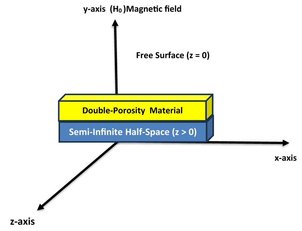
Geometry of the problem.
The equations and relations that describe the behavior of a thermoelastic solid with a double-porosity structure, which is both homogenous and isotropic, in the presence of a magnetic field and without any additional forces or heat sources, are provided by the L-S model:
Equations for double porosity [35]:
Equilibrated stress equations of motion [35]:
For simplicity, we introduce the following dimensionless variables [37,38]:
Using the above dimensionless quantities, Eqs. (8)–(13) become
The stress components can be expressed in dimensionless variables in the following manner:
where
We define the displacement potentials
Using Eq. (23) in Eqs. (14)–(18), we obtain
3 Normal mode analysis
The solution of the given physical variable can be expressed as the decomposition in terms of normal modes (derived by assuming exponential representations), as follows [40,41]:
where
Using (29) in Eqs. (19)–(22) and Eqs. (24)–(28) we obtain
where
Eliminating
where
Technical factors were used to solve the main ordinary differential equation (ODE) (36) as follows:
where
In the same way, the solutions of the other quantities can be expressed as follows:
Since
Then,
The stress components can be expressed using dimensionless variables. By substituting the stress displacement from Eqs. (51) and (52) into Eqs. (20)–(22), we obtain the components in the following form:
The dimensionless variables for the components of
where
To obtain the solution of
where
The solutions to the major variables that transform the domain in terms of unknown parameters
4 Boundary conditions
We apply six boundary conditions for the present problem at the plane surface
Substituting Eqs. (60)–(65) in (43), (44), (53), (55), (56), and (57), we obtain
To obtain
5 Numerical results
The effect of a magnetic field on double porosity is now investigated, and numerical findings are presented. Silicon is chosen as the thermoelastic material, and the following values of physical constants are employed to attain this purpose [26,27].
Following Khalili [35], the double porous parameters are considered as
To solve the issue, we utilized the numerical technique described above to distribute the real part of the temperature
Figure 2 shows a comparison between the three different values of the thermoelastic coupling parameter
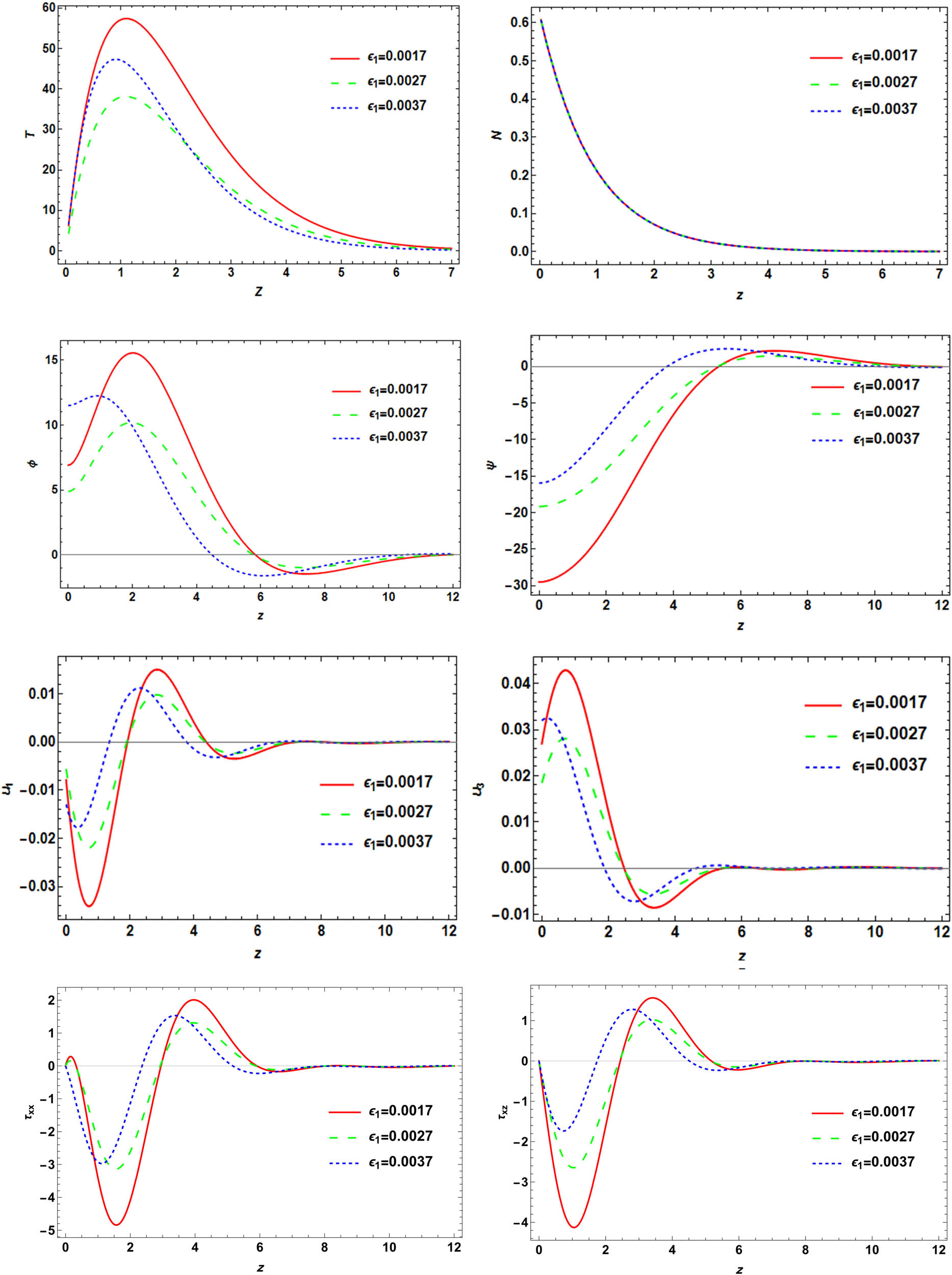
Variation of physical field distributions with distance at different thermoelastic coupling parameter
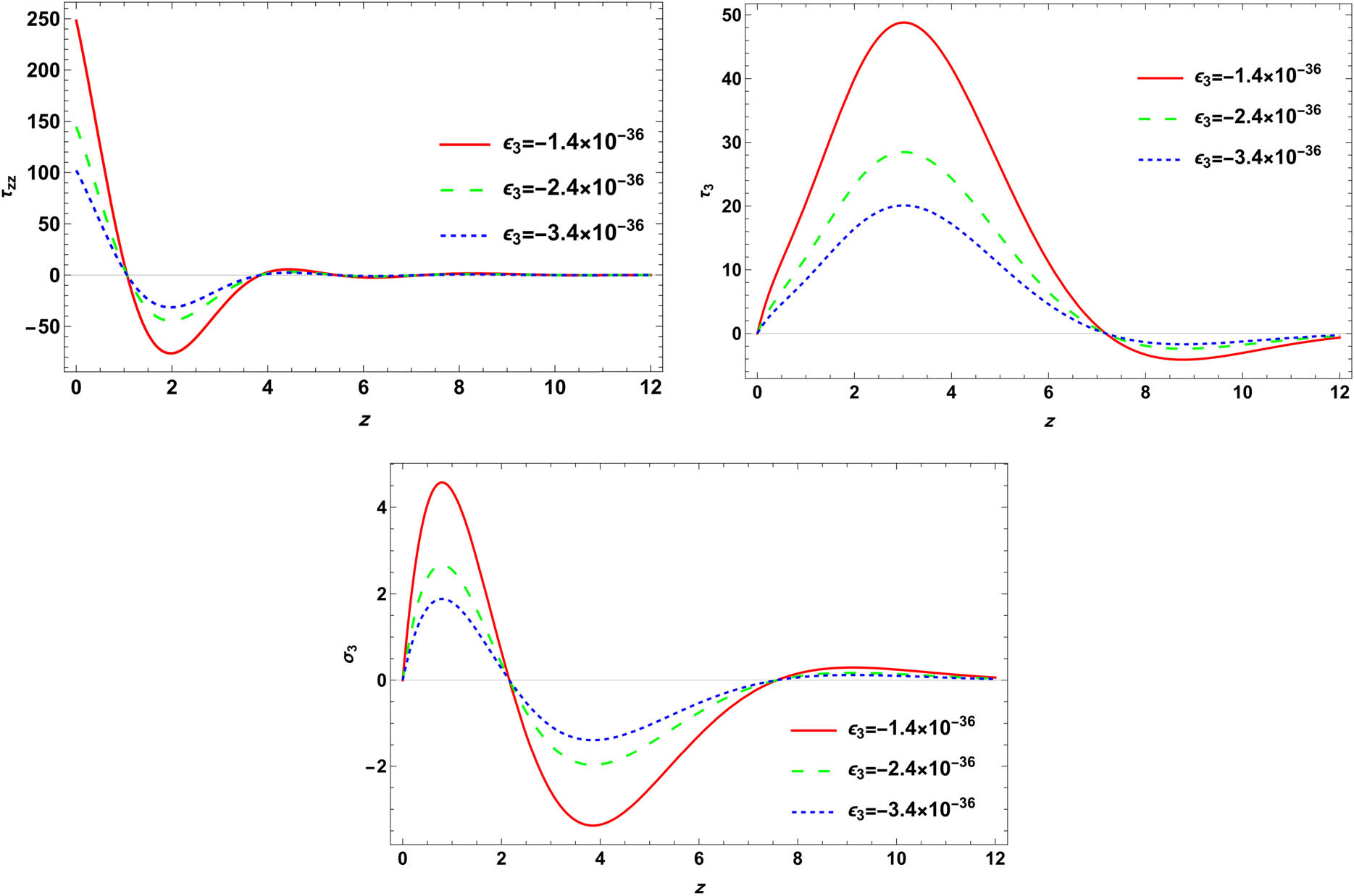
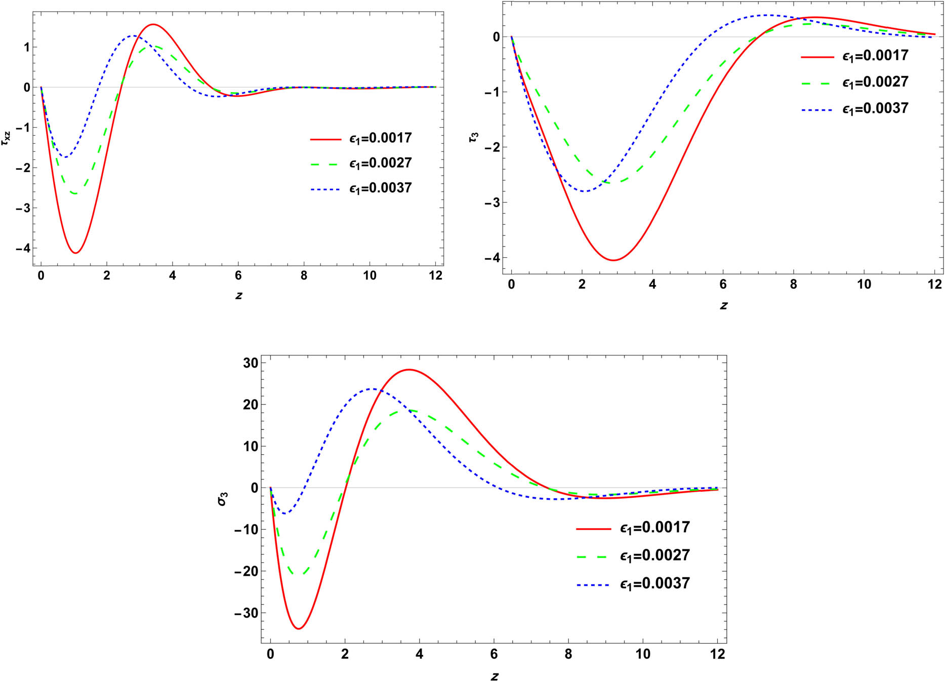
Variation in physical field distributions with distance at different thermoelectric
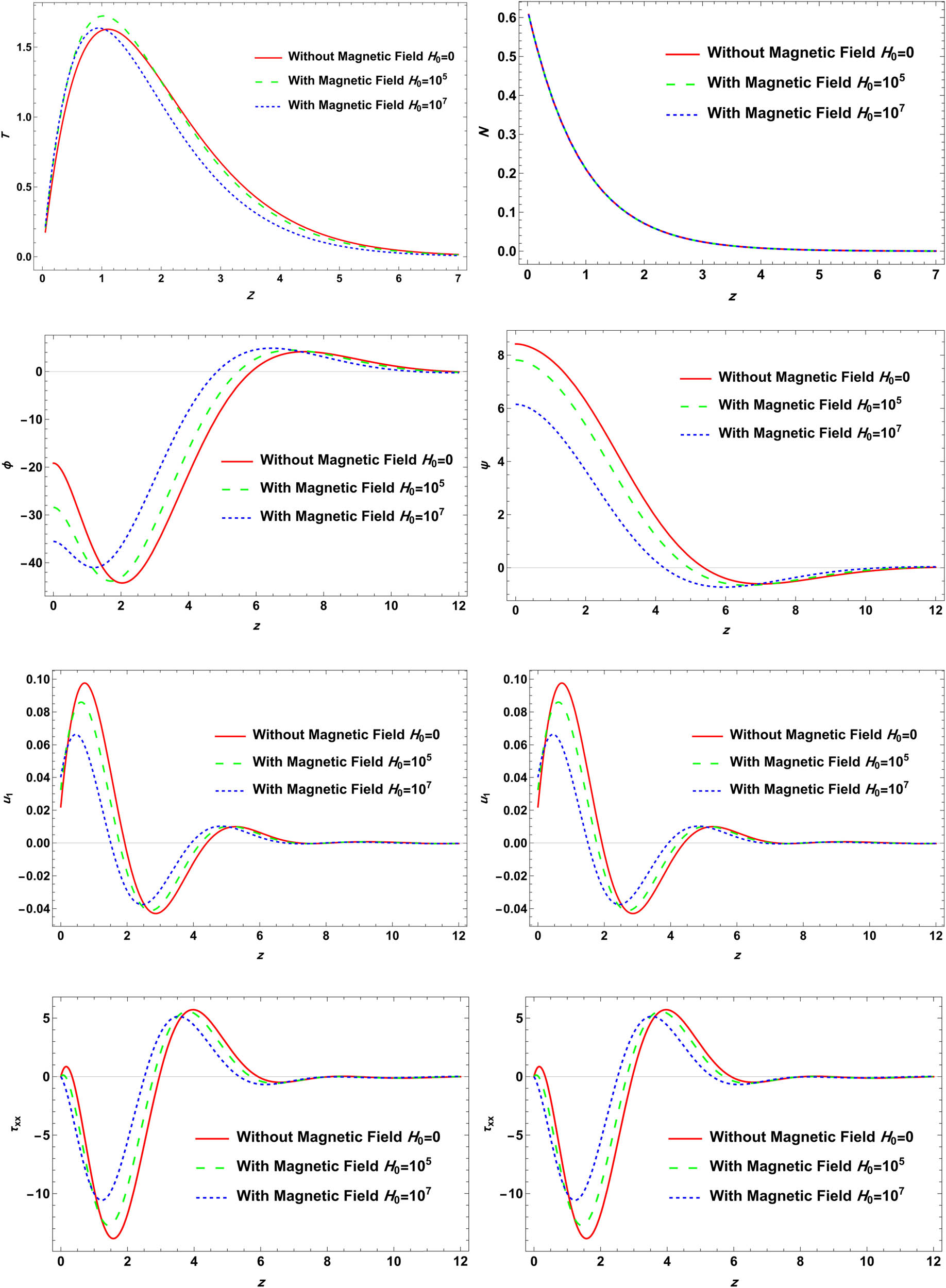
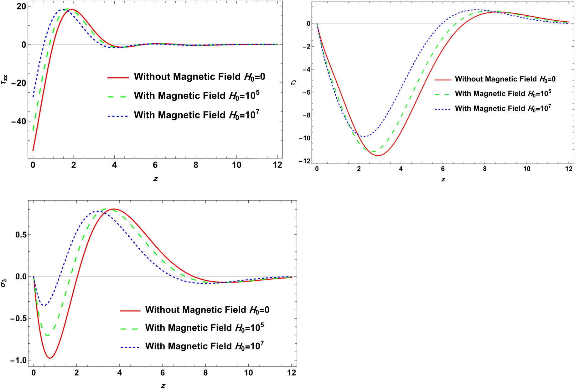
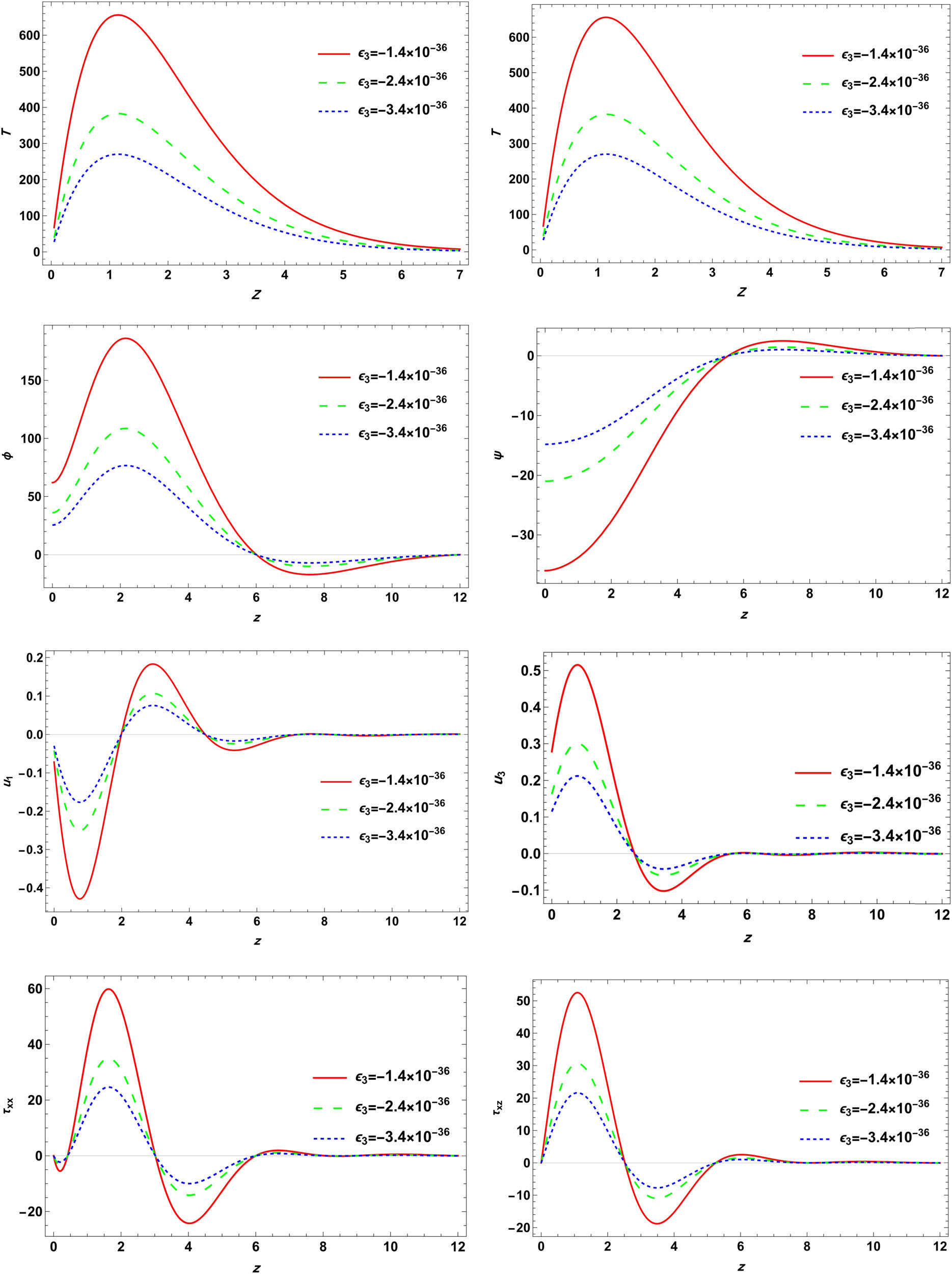
Variation in physical field distributions with distance at different magnetic field


3D graphs of physical field distributions with distance and time.

Heat map for temperature and stress distributions.
5.1 Validation
To ensure the accuracy and reliability of the proposed model, we validate our numerical results by comparing them with the existing theoretical and experimental data from the literature (Table 1). Specifically, we compare our results with those obtained in previous studies that analyze similar thermoelastic and double-porosity systems [42].
Comparison of numerical results with previous studies
| Study | Considered effects | Key findings | Agreement with present work |
|---|---|---|---|
| Abdou et al. [44] | Double porosity, no magnetic field | Thermoelastic behavior in double-porous media | Strong agreement |
| Lotfy et al. [42] | No magnetic field, no double porosity | Classical photo-thermoelastic response | Strong agreement |
| Present study | Magnetic field, double porosity | Magneto-photo-thermoelastic interactions |
First, when the magnetic field parameter is set to zero, our results align closely with those reported by Abdou et al. [43], who studied generalized thermoelastic media with double porosity under the L-S’s theory. This confirms the consistency of our model in the absence of an external magnetic field.
Furthermore, if both the magnetic field and the double-porosity effects are neglected, our findings reduce to the results obtained by Lotfy et al. [42] in the context of classical photo-thermoelasticity. The agreement between these cases demonstrates the robustness and adaptability of our model under different physical conditions.
The numerical comparisons indicate that the computed results, including displacement, stress, temperature, and porosity variations, exhibit a strong correlation with previously established findings. This validation confirms the effectiveness of our analytical approach and numerical implementation in capturing the complex interactions of thermoelasticity, magnetoelasticity, and double-porosity effects in semiconductor materials.
By successfully reproducing known results in limiting cases, our study provides confidence in the applicability of the proposed model for analyzing magneto-photo-thermoelastic interactions in double-porous media.
Table 1 highlights the consistency of our results with previous studies, reinforcing the validity of our model and its applicability to different physical scenarios.
6 Discussion and conclusion
The study has examined a novel mathematical model of the L-S theory within photo-thermoelastic theory, considering the effects of the magnetic field and double porosity. The research investigates the impact of thermoelastic and thermoelectric coupling parameters and magnetic fields on various physical phenomena within the problem. The external magnetic field affects the transmission of fundamental physical fields. The propagation of waves is regulated by the interplay of coupled photo-thermoelasticity, magnetic fields, dual porosity, and the physical constants of the material. The relationship between thermoelastic and thermoelectric properties is evident within the framework of photo-thermoelastic theory.
To enhance the analysis, logarithmic scaling has been introduced in Figure 2 for the horizontal axis, allowing a more comprehensive visualization of parameter variations across different scales. The application of a logarithmic transformation is particularly useful for capturing variations in temperature and stress distributions over a wide range, aligning with similar methodologies presented in recent studies, such as Seem and Singhal [27]. The logarithmic scale improves the clarity of trends in regions where small-scale behavior is critical, thereby enhancing the interpretability of the graphical results.
6.1 Clarification of double porosity
In this study, double porosity refers to a material possessing two distinct pore systems, typically classified as macropores and microfissures. Macropores are larger cavities that dominate bulk fluid flow, while microfissures are smaller cracks or pores within the material. This dual-porosity structure leads to complex mechanical and thermal responses, affecting how waves propagate and stress is distributed within the material [44,45].
The presence of double porosity significantly influences the behavior of materials in engineering and geophysical applications. In porous geological formations, such as oil reservoirs and aquifers, the interaction between macropores and microfissures controls fluid transport, stress distribution, and wave propagation, making this concept crucial for enhancing oil recovery and geothermal energy extraction. Similarly, in biomedical engineering, porous materials with double porosity are used in bone implants and tissue scaffolds, where controlling the mechanical properties and fluid permeability is essential for biological integration. Furthermore, in semiconductor and nanotechnology applications, structured porous materials play a key role in thermal management and electronic cooling systems. By incorporating double porosity into our analysis, this study provides a deeper understanding of wave interactions in complex media, offering insights applicable to diverse scientific and industrial fields [46–48].
Furthermore, we analyze the physical significance of the studied parameters and their impact on the half-space behavior:
Thermoelastic and thermoelectric coupling: The thermoelastic coupling parameter governs the interaction between thermal and mechanical fields. Higher values lead to increased thermal stresses and temperature gradients, causing stronger mechanical deformations. This behavior is particularly relevant in applications such as geothermal energy extraction and high-temperature electronic materials, where managing thermal expansion is crucial.
Magnetic field influence: The applied magnetic field introduces Lorentz forces, which act as a damping mechanism on mechanical oscillations and wave propagation. This effect is critical in semiconductor applications and electromagnetic shielding materials, where reducing unwanted vibrations enhances stability and performance.
Double porosity and wave propagation: The presence of two distinct pore systems significantly modifies wave speeds and stress distributions. This insight is essential for oil reservoir modeling and carbon sequestration, where understanding wave behavior in porous formations can optimize resource extraction techniques.
Geometrical considerations: The depth and spatial extent of porosity variations influence stress concentrations and fracture propagation. This effect is particularly relevant in earthquake modeling and rock mechanics, where stress accumulation can lead to seismic activity and structural failures.
6.2 Real-world applications
The findings of this study have significant implications in various engineering and technological domains, including:
Geophysics and earthquake engineering: Understanding wave propagation in double-porous materials helps improve seismic wave analysis and earthquake prediction models, which are critical for designing safer infrastructure in earthquake-prone regions.
Oil and gas industry: The study provides insights into fluid dynamics in reservoir rocks, enhancing techniques for oil recovery and carbon sequestration by modeling how waves and stresses interact in porous geological formations.
Semiconductor and nanotechnology: The integration of magneto-photo-thermoelastic effects is valuable for optimizing semiconductor devices, including photonic and optoelectronic sensors used in precision applications.
Biomedical engineering: Double-porosity structures with thermoelastic properties can be utilized in biomedical implants, particularly for materials that require enhanced stress distribution and controlled thermal expansion.
Aerospace and structural health monitoring: Magnetic and thermal effects in porous materials play a crucial role in the design of lightweight, thermally stable materials for aerospace structures and real-time structural health monitoring systems.
Neglecting the effects of the external magnetic field and photothermal stimulation, the research findings underscore the importance of thermoelectric, thermoelastic, and magnetic fields in various modern geophysical engineering applications, such as solar cells, display technologies, and electrical circuits. Magnetic fields substantially influence the precision of measuring displacement, tension, and strain. Phase delays substantially affect all distributions [48,49].
The main aim of this work is to examine the effect of a magnetic field on a medium characterized by dual porosity levels, particularly with L-S’s theory. The investigation aims to determine the extent to which the magnetic field influences the amplitude of certain physical parameters, either by enhancing or diminishing them. The data were acquired by contrasting the twofold porosity with and without a magnetic field. This comparison unveiled noteworthy instances. The normal mode method has been utilized to ascertain general solutions, which yield accurate responses by converting partial differential equations into ordinary differential equations through the implementation of boundary conditions. Programming enables us to observe the functionality of functions at certain values. The MATHEMATICA program was used to calculate numerical solutions. When exposed to a magnetic field, the differences between the existence and non-existence of double porosity are significant. All the physical quantities satisfy the boundary requirements. All physical quantities tend towards zero, and all functions exhibit continuity.
While this problem is theoretical, it can provide useful insights for experimental researchers in the domains of geophysics, earthquake engineering, and seismology, especially those who are studying mining tremors and drilling into the Earth’s crust. Applying numerical approaches to solve the system of equations and conditions that govern the phenomenon can help overcome the limitations of the normal modes technique. This undertaking is currently in progress. The importance of this problem lies in its potential to improve our understanding of complex material behaviors, leading to innovations in the design and application of advanced materials in a variety of high-tech fields.
We examined the thermoelastic and fluid flow behavior of a double-porosity material under a magnetic field and the effects of many dominant factors. The parameters include thermoelastic, thermoelectric, and magnetic field intensity coupling parameters. First, thermal and elastic fields interact via the thermoelastic coupling parameter. Our results indicate that higher values increase thermal stresses and temperature-deformation field coupling. This increases displacement amplitudes and stress concentrations at the free surface. Geothermal energy extraction materials with higher porosity are more vulnerable to heat cracking, which improves the fracture fluid flow. Controlling helps biomedical device materials like thermal actuators and sensors respond reliably to thermal stimuli. Second, the thermoelectric coupling parameter controls the thermal–electric field interaction. We found that higher values increase thermal energy conversion into electric energy, carrier density (N), and heat transfer. Semiconducting materials, where thermoelectric coupling is crucial to energy harvesting, exhibit this phenomenon. Optimization improves thermal-to-electric energy conversion in solar cells. In electronic cooling systems, customized materials improve heat dissipation and prevent overheating. Finally, through the Lorentz force and induced electric fields, the magnetic field intensity greatly affects the material reaction. Our study shows that the opposing Lorentz force dampens elastic waves and reduces displacement amplitudes. Higher magnetic fields reduce stress concentrations at the free surface. Magnetic field sensors use controlled materials to detect and quantify magnetic fields precisely. Aerospace engineering uses magnetic fields to stabilize thermal and mechanical loads.
Acknowledgments
The authors would like to extend their sincere appreciation to Ongoing Research Funding program (ORF-2025-1112), King Saud University, Riyadh, Saudi Arabia.
-
Funding information: The project was funded under Project number (ORF-2025-1112).
-
Author contributions: All authors have accepted responsibility for the entire content of this manuscript and approved its submission.
-
Conflict of interest: The authors state no conflict of interest.
-
Data availability statement: The datasets generated and/or analyzed during the current study are available from the corresponding author on reasonable request.
References
[1] Biot MA. Mechanics of deformation and acoustic propagation in porous media. J Appl Phys. 1962;33(4):1482–98. 10.1063/1.1728759.Search in Google Scholar
[2] Detournay E, Cheng AHD. Fundamentals of poroelasticity. Compr Rock Eng: Princ Pract Proj. 1993;2:113–71.10.1016/B978-0-08-040615-2.50011-3Search in Google Scholar
[3] Pal SK, Maiti S. Thermoelastic response of a thin circular disk of double porosity under axisymmetric thermal shock. J Therm Stresses. 2001;24(6):509–28. 10.1080/014957301300004494.Search in Google Scholar
[4] Rice JR, Cleary MP. Some basic stress diffusion solutions for fluid-saturated elastic porous media with compressible constituents. Rev Geophys Space Phys. 1976;14(2):227–41. 10.1029/RG014i002p00227.Search in Google Scholar
[5] Zhao J, Wang Y. Photothermoelastic analysis of a multilayered composite cylinder with functionally graded material and double porosity. Int J Mech Sci. 2020;184:105763. 10.1016/j.ijmecsci.2020.105763.Search in Google Scholar
[6] Lord H, Shulman Y. A generalized dynamical theory of thermoelasticity. J Mech Phys Solids. 1967;15:299–309.10.1016/0022-5096(67)90024-5Search in Google Scholar
[7] Barrenblatt G, Zheltov I, Kockina I. Basic concepts in the theory of seepage of homogeneous liquids in fissured rocks (Strata). Prikl Mat Mekh (Engl Translation). 1960;24:1286–303.10.1016/0021-8928(60)90107-6Search in Google Scholar
[8] Barrenblatt G, Zheltov I. On the basic equations of seepage of homogeneous liquids in fissured rock. Akad Nauk SSSR (Engl Translation). 1960;132:545–8.Search in Google Scholar
[9] Khalili N, Valliappan S. Unified theory of flow and deformation in double porous media. Eur J Mech A, Solids. 1996;15:321–36.Search in Google Scholar
[10] Masters I, Pao W, Lewis R. Coupling temperature to a double-porosity model of deformable porous media. Int J Numer Methods Eng. 2000;49:421–38.10.1002/1097-0207(20000930)49:3<421::AID-NME48>3.3.CO;2-YSearch in Google Scholar
[11] Khalili N, Selvadurai A. A fully coupled constitutive model for thermo-hydro-mechanical analysis in elastic media with double porosity. Geophys Res Lett. 2003;30(24):2268.10.1029/2003GL018838Search in Google Scholar
[12] Zhao Y, Chen M. Fully coupled dual-porosity model for anisotropic formations. Int J Rock Mech Min Sci. 2006;43(7):1128–33.10.1016/j.ijrmms.2006.03.001Search in Google Scholar
[13] Svanadze M. Dynamical problems of the theory of elasticity for solids with double porosity. Proc Appl Math Mech. 2010;10:309–10.10.1002/pamm.201010147Search in Google Scholar
[14] Ainouz A. Homogenized double porosity models for poro-elastic media with interfacial flow barrier. Math Bohem. 2011;136:357–65.10.21136/MB.2011.141695Search in Google Scholar
[15] Svanadze M. Plane waves and boundary value problems in the theory of elasticity for solids with double porosity. Acta Appl Math. 2012;122:461–71.10.1007/s10440-012-9756-5Search in Google Scholar
[16] Straughan B. Stability and uniqueness in double porosity elasticity. Int J Eng Sci. 2013;65:1–8.10.1016/j.ijengsci.2013.01.001Search in Google Scholar
[17] Mahato CS, Biswas S. State space approach to characterize Rayleigh waves in nonlocal thermoelastic medium with double porosity under three-phase-lag model. Comput Math Math Phys. 2024;64(3):555–84.10.1134/S0965542524030060Search in Google Scholar
[18] Berryman JG, Wang HF. The elastic coefficients of double-porosity models for fluid transport in jointed rock. J Geophys Res: Solid Earth. 1995;100(B12):24611–27. 10.1029/95JB02665.Search in Google Scholar
[19] Lewis RW, Schrefler BA. The finite element method in the deformation and consolidation of porous media. New York: John Wiley & Sons; 1998.Search in Google Scholar
[20] Marin M, Marinescu C. Thermoelasticity of initially stressed bodies, asymptotic equipartition of energies. Int J Eng Sci. 1998;36(1):73–86.10.1016/S0020-7225(97)00019-0Search in Google Scholar
[21] Florea OA. The backward-in-time problem of double porosity material with microtemperature. Symmetry. 2019;11(4):552.10.3390/sym11040552Search in Google Scholar
[22] Kumar D, Singh D, Tomar SK. Surface waves in layered thermoelastic medium with double porosity structure: Rayleigh and Stoneley waves. Mech Adv Mater Struct. 2022;29(18):2680–705.10.1080/15376494.2021.1876283Search in Google Scholar
[23] Arusoaie A. Spatial and temporal behavior in the theory of thermoelasticity for solids with double porosity. J Therm Stresses. 2018;41(4):500–21.10.1080/01495739.2017.1387882Search in Google Scholar
[24] Rana N, Sharma DK, Sharma SR, Sarkar N. Effect of electromagnetic field on vibrations of nonlocal elastic cylinders with double porosity. J Vib Eng Technol. 2024;12(1):427–39. 10.1007/s42417-024-01424-x Search in Google Scholar
[25] Kumar R, Vohra R. Response of thermoelastic microbeam with double porosity structure due to pulsed laser heating. Mech Mech Eng. 2019;23(1).10.2478/mme-2019-0011Search in Google Scholar
[26] Seema S, Singhal A. Study of surface wave velocity in distinct rheological models with flexoelectric effect in piezoelectric aluminium nitride structure. J Braz Soc Mech Sci Eng. 2025;47:29. 10.1007/s40430-024-05296-w.Search in Google Scholar
[27] Seema S, Singhal A. Examining three distinct rheological models with flexoelectric effect to investigate Love-type wave velocity in bedded piezo-structure. Z Angew Math Mech. 2024;104:202400724. 10.1002/zamm.202400724.Search in Google Scholar
[28] Seema S, Singhal A. Mechanics of SH and anti-plane SH waves in orthotropic piezoelectric quasicrystal with multiple surface effect. Acta Mech. 2025;236:439–56. 10.1007/s00707-024-04162-z.Search in Google Scholar
[29] Seema S, Singhal A. Surface effects study: a continuum approach from fundamental modes to higher modes and topological polarization in orthotropic piezoelectric materials. J Appl Mech. 2025;92(1):011008. 10.1115/1.4067204.Search in Google Scholar
[30] Oreyeni T, Shamshuddin M, Obalalu A, Saeed A, Shah N. Exploring the impact of stratification on the dynamics of bioconvective thixotropic fluid conveying tiny particles and Cattaneo-Christov model: Thermal storage system application. Propuls Power Res. 2024;13(3):416–32. 10.1016/j.jppr.2024.08.002.Search in Google Scholar
[31] Shamshuddin M, Panda S, Pattnaik P, Mishra S. Ferromagnetic and Ohmic effects on nanofluid flow via permeability rotative disk: significant interparticle radial and nanoparticle radius. Phys Scr. 2024;99:055206. 10.1088/1402-4896/ad35f8.Search in Google Scholar
[32] Lotfy K, Elidy ES, Tantawi RS. Photothermal excitation process during hyperbolic two-temperature theory for magneto-thermo-elastic semiconducting medium. Silicon. 2021;13:2275–88.10.1007/s12633-020-00795-6Search in Google Scholar
[33] El-Sapa S, Lotfy K, Elidy ES, El-Bary A, Tantawi RS. Photothermal excitation process in semiconductor materials under the effect moisture diffusivity. Silicon. 2023;15(10):4171–82.Search in Google Scholar
[34] El-Sapa S, Lotfy K, Elidy ES, Tantawi RS. Photothermal excitation process in semiconductor materials under the effect moisture diffusivity. Silicon. 2023;15:4171–82. 10.1007/s12633-023-02311-y.Search in Google Scholar
[35] Khalili N. Coupling effects in double porosity media with deformable matrix. Geo Res Lett. 2003;30(22):2153–5.10.1029/2003GL018544Search in Google Scholar
[36] Ieşan D, Quintanilla R. On a theory of thermoelastic materials with a double porosity structure. J Therm Stress. 2014;37:1017–36.10.1080/01495739.2014.914776Search in Google Scholar
[37] Marin M, Lupu M. On harmonic vibrations in thermoelasticity of micropolar bodies. J Vib Control. 1998;4(5):507–18. 10.1177/107754639800400501.Search in Google Scholar
[38] Marin M, Abbas I, Kumar R. Relaxed Saint-Venant principle for thermoelastic micropolar diffusion. Struct Eng Mech. 2014;51(4):651–62.10.12989/sem.2014.51.4.651Search in Google Scholar
[39] Marin M. Lagrange identity method for microstretch thermoelastic materials. J Math Anal Appl. 2010;363(1):275–86. 10.1016/j.jmaa.2009.08.045.Search in Google Scholar
[40] Bhatti MM, Marin M, Ellahi R, Fudulu IM. Insight into the dynamics of EMHD hybrid nanofluid (ZnO/CuO-SA) flow through a pipe for geothermal energy applications. J Therm Anal Calorim. 2023;148:14261–73. 10.1007/s10973-023-12565-8.Search in Google Scholar
[41] Yadav A, Carrera E, Marin M, Othman M. Reflection of hygrothermal waves in a Nonlocal Theory of coupled thermo-elasticity. Mech Adv Mater Struct. 2024;31(5):1083–96. 10.1080/15376494.2024.Search in Google Scholar
[42] Lotfy K, Mahdy AMS, El-Bary AA, Elidy ES. Magneto-photo-thermoelastic excitation rotating semiconductor medium based on moisture diffusivity. CMES-Comput Model Eng Sci. 2024;141(1):107–26.10.32604/cmes.2024.053199Search in Google Scholar
[43] Abdou MA, Othman MI, Tantawi RS, Mansour NT. Exact solutions of generalized thermoelastic medium with double porosity under L–S theory. Indian J Phys. 2020;94:725–36.10.1007/s12648-019-01505-8Search in Google Scholar
[44] Abdou MA, Othman MI, Tantawi RS, Mansour NT. Effect of magnetic field on generalized thermoelastic medium with double porosity structure under L–S theory. Indian J Phys. 2020;94:1993–2004.10.1007/s12648-019-01648-8Search in Google Scholar
[45] Aljadani MH, Zenkour AM. Effect of magnetic field on a thermoviscoelastic body via a refined two-temperature Lord–Shulman model. Case Stud Therm Eng. 2023;49:103197. 10.1016/j.csite.2023.103197.Search in Google Scholar
[46] Heydarpour Y, Malekzadeh P, Gholipour F. Thermoelastic analysis of FG-GPLRC spherical shells under thermo-mechanical loadings based on Lord-Shulman theory. Compos Part B: Eng. 2019;164:400–24. 10.1016/j.compositesb.2018.12.073.Search in Google Scholar
[47] Kheibari F, Beni YT, Golestanian H. On the generalized flexothermoelasticity of a microlayer. Acta Mech. 2024;235:3363–84. 10.1007/s00707-024-03884-4.Search in Google Scholar
[48] Pakdaman M, Tadi Beni Y. Size-dependent Generalized Piezothermoelasticity of Microlayer. J Appl Comput Mech. 2025;11(1):223–38. 10.22055/jacm.2024.46393.4510.Search in Google Scholar
[49] Kheibari F, Beni YT, Kiani Y. Lord-Shulman based generalized thermoelasticity of piezoelectric layer using finite element method. Struct Eng Mech. 2024;92(1):81–8. 10.12989/sem.2024.92.1.081.Search in Google Scholar
© 2025 the author(s), published by De Gruyter
This work is licensed under the Creative Commons Attribution 4.0 International License.
Articles in the same Issue
- Research Articles
- Single-step fabrication of Ag2S/poly-2-mercaptoaniline nanoribbon photocathodes for green hydrogen generation from artificial and natural red-sea water
- Abundant new interaction solutions and nonlinear dynamics for the (3+1)-dimensional Hirota–Satsuma–Ito-like equation
- A novel gold and SiO2 material based planar 5-element high HPBW end-fire antenna array for 300 GHz applications
- Explicit exact solutions and bifurcation analysis for the mZK equation with truncated M-fractional derivatives utilizing two reliable methods
- Optical and laser damage resistance: Role of periodic cylindrical surfaces
- Numerical study of flow and heat transfer in the air-side metal foam partially filled channels of panel-type radiator under forced convection
- Water-based hybrid nanofluid flow containing CNT nanoparticles over an extending surface with velocity slips, thermal convective, and zero-mass flux conditions
- Dynamical wave structures for some diffusion--reaction equations with quadratic and quartic nonlinearities
- Solving an isotropic grey matter tumour model via a heat transfer equation
- Study on the penetration protection of a fiber-reinforced composite structure with CNTs/GFP clip STF/3DKevlar
- Influence of Hall current and acoustic pressure on nanostructured DPL thermoelastic plates under ramp heating in a double-temperature model
- Applications of the Belousov–Zhabotinsky reaction–diffusion system: Analytical and numerical approaches
- AC electroosmotic flow of Maxwell fluid in a pH-regulated parallel-plate silica nanochannel
- Interpreting optical effects with relativistic transformations adopting one-way synchronization to conserve simultaneity and space–time continuity
- Modeling and analysis of quantum communication channel in airborne platforms with boundary layer effects
- Theoretical and numerical investigation of a memristor system with a piecewise memductance under fractal–fractional derivatives
- Tuning the structure and electro-optical properties of α-Cr2O3 films by heat treatment/La doping for optoelectronic applications
- High-speed multi-spectral explosion temperature measurement using golden-section accelerated Pearson correlation algorithm
- Dynamic behavior and modulation instability of the generalized coupled fractional nonlinear Helmholtz equation with cubic–quintic term
- Study on the duration of laser-induced air plasma flash near thin film surface
- Exploring the dynamics of fractional-order nonlinear dispersive wave system through homotopy technique
- The mechanism of carbon monoxide fluorescence inside a femtosecond laser-induced plasma
- Numerical solution of a nonconstant coefficient advection diffusion equation in an irregular domain and analyses of numerical dispersion and dissipation
- Numerical examination of the chemically reactive MHD flow of hybrid nanofluids over a two-dimensional stretching surface with the Cattaneo–Christov model and slip conditions
- Impacts of sinusoidal heat flux and embraced heated rectangular cavity on natural convection within a square enclosure partially filled with porous medium and Casson-hybrid nanofluid
- Stability analysis of unsteady ternary nanofluid flow past a stretching/shrinking wedge
- Solitonic wave solutions of a Hamiltonian nonlinear atom chain model through the Hirota bilinear transformation method
- Bilinear form and soltion solutions for (3+1)-dimensional negative-order KdV-CBS equation
- Solitary chirp pulses and soliton control for variable coefficients cubic–quintic nonlinear Schrödinger equation in nonuniform management system
- Influence of decaying heat source and temperature-dependent thermal conductivity on photo-hydro-elasto semiconductor media
- Dissipative disorder optimization in the radiative thin film flow of partially ionized non-Newtonian hybrid nanofluid with second-order slip condition
- Bifurcation, chaotic behavior, and traveling wave solutions for the fractional (4+1)-dimensional Davey–Stewartson–Kadomtsev–Petviashvili model
- New investigation on soliton solutions of two nonlinear PDEs in mathematical physics with a dynamical property: Bifurcation analysis
- Mathematical analysis of nanoparticle type and volume fraction on heat transfer efficiency of nanofluids
- Creation of single-wing Lorenz-like attractors via a ten-ninths-degree term
- Optical soliton solutions, bifurcation analysis, chaotic behaviors of nonlinear Schrödinger equation and modulation instability in optical fiber
- Chaotic dynamics and some solutions for the (n + 1)-dimensional modified Zakharov–Kuznetsov equation in plasma physics
- Fractal formation and chaotic soliton phenomena in nonlinear conformable Heisenberg ferromagnetic spin chain equation
- Single-step fabrication of Mn(iv) oxide-Mn(ii) sulfide/poly-2-mercaptoaniline porous network nanocomposite for pseudo-supercapacitors and charge storage
- Novel constructed dynamical analytical solutions and conserved quantities of the new (2+1)-dimensional KdV model describing acoustic wave propagation
- Tavis–Cummings model in the presence of a deformed field and time-dependent coupling
- Spinning dynamics of stress-dependent viscosity of generalized Cross-nonlinear materials affected by gravitationally swirling disk
- Design and prediction of high optical density photovoltaic polymers using machine learning-DFT studies
- Robust control and preservation of quantum steering, nonlocality, and coherence in open atomic systems
- Coating thickness and process efficiency of reverse roll coating using a magnetized hybrid nanomaterial flow
- Dynamic analysis, circuit realization, and its synchronization of a new chaotic hyperjerk system
- Decoherence of steerability and coherence dynamics induced by nonlinear qubit–cavity interactions
- Finite element analysis of turbulent thermal enhancement in grooved channels with flat- and plus-shaped fins
- Modulational instability and associated ion-acoustic modulated envelope solitons in a quantum plasma having ion beams
- Statistical inference of constant-stress partially accelerated life tests under type II generalized hybrid censored data from Burr III distribution
- On solutions of the Dirac equation for 1D hydrogenic atoms or ions
- Entropy optimization for chemically reactive magnetized unsteady thin film hybrid nanofluid flow on inclined surface subject to nonlinear mixed convection and variable temperature
- Stability analysis, circuit simulation, and color image encryption of a novel four-dimensional hyperchaotic model with hidden and self-excited attractors
- A high-accuracy exponential time integration scheme for the Darcy–Forchheimer Williamson fluid flow with temperature-dependent conductivity
- Novel analysis of fractional regularized long-wave equation in plasma dynamics
- Development of a photoelectrode based on a bismuth(iii) oxyiodide/intercalated iodide-poly(1H-pyrrole) rough spherical nanocomposite for green hydrogen generation
- Investigation of solar radiation effects on the energy performance of the (Al2O3–CuO–Cu)/H2O ternary nanofluidic system through a convectively heated cylinder
- Quantum resources for a system of two atoms interacting with a deformed field in the presence of intensity-dependent coupling
- Studying bifurcations and chaotic dynamics in the generalized hyperelastic-rod wave equation through Hamiltonian mechanics
- A new numerical technique for the solution of time-fractional nonlinear Klein–Gordon equation involving Atangana–Baleanu derivative using cubic B-spline functions
- Interaction solutions of high-order breathers and lumps for a (3+1)-dimensional conformable fractional potential-YTSF-like model
- Hydraulic fracturing radioactive source tracing technology based on hydraulic fracturing tracing mechanics model
- Numerical solution and stability analysis of non-Newtonian hybrid nanofluid flow subject to exponential heat source/sink over a Riga sheet
- Numerical investigation of mixed convection and viscous dissipation in couple stress nanofluid flow: A merged Adomian decomposition method and Mohand transform
- Effectual quintic B-spline functions for solving the time fractional coupled Boussinesq–Burgers equation arising in shallow water waves
- Analysis of MHD hybrid nanofluid flow over cone and wedge with exponential and thermal heat source and activation energy
- Solitons and travelling waves structure for M-fractional Kairat-II equation using three explicit methods
- Impact of nanoparticle shapes on the heat transfer properties of Cu and CuO nanofluids flowing over a stretching surface with slip effects: A computational study
- Computational simulation of heat transfer and nanofluid flow for two-sided lid-driven square cavity under the influence of magnetic field
- Irreversibility analysis of a bioconvective two-phase nanofluid in a Maxwell (non-Newtonian) flow induced by a rotating disk with thermal radiation
- Hydrodynamic and sensitivity analysis of a polymeric calendering process for non-Newtonian fluids with temperature-dependent viscosity
- Exploring the peakon solitons molecules and solitary wave structure to the nonlinear damped Kortewege–de Vries equation through efficient technique
- Modeling and heat transfer analysis of magnetized hybrid micropolar blood-based nanofluid flow in Darcy–Forchheimer porous stenosis narrow arteries
- Activation energy and cross-diffusion effects on 3D rotating nanofluid flow in a Darcy–Forchheimer porous medium with radiation and convective heating
- Insights into chemical reactions occurring in generalized nanomaterials due to spinning surface with melting constraints
- Influence of a magnetic field on double-porosity photo-thermoelastic materials under Lord–Shulman theory
- Soliton-like solutions for a nonlinear doubly dispersive equation in an elastic Murnaghan's rod via Hirota's bilinear method
- Analytical and numerical investigation of exact wave patterns and chaotic dynamics in the extended improved Boussinesq equation
- Nonclassical correlation dynamics of Heisenberg XYZ states with (x, y)-spin--orbit interaction, x-magnetic field, and intrinsic decoherence effects
- Exact traveling wave and soliton solutions for chemotaxis model and (3+1)-dimensional Boiti–Leon–Manna–Pempinelli equation
- Unveiling the transformative role of samarium in ZnO: Exploring structural and optical modifications for advanced functional applications
- On the derivation of solitary wave solutions for the time-fractional Rosenau equation through two analytical techniques
- Analyzing the role of length and radius of MWCNTs in a nanofluid flow influenced by variable thermal conductivity and viscosity considering Marangoni convection
- Advanced mathematical analysis of heat and mass transfer in oscillatory micropolar bio-nanofluid flows via peristaltic waves and electroosmotic effects
- Exact bound state solutions of the radial Schrödinger equation for the Coulomb potential by conformable Nikiforov–Uvarov approach
- Some anisotropic and perfect fluid plane symmetric solutions of Einstein's field equations using killing symmetries
- Nonlinear dynamics of the dissipative ion-acoustic solitary waves in anisotropic rotating magnetoplasmas
- Curves in multiplicative equiaffine plane
- Exact solution of the three-dimensional (3D) Z2 lattice gauge theory
- Propagation properties of Airyprime pulses in relaxing nonlinear media
- Symbolic computation: Analytical solutions and dynamics of a shallow water wave equation in coastal engineering
- Wave propagation in nonlocal piezo-photo-hygrothermoelastic semiconductors subjected to heat and moisture flux
- Comparative reaction dynamics in rotating nanofluid systems: Quartic and cubic kinetics under MHD influence
- Laplace transform technique and probabilistic analysis-based hypothesis testing in medical and engineering applications
- Physical properties of ternary chloro-perovskites KTCl3 (T = Ge, Al) for optoelectronic applications
- Gravitational length stretching: Curvature-induced modulation of quantum probability densities
- The search for the cosmological cold dark matter axion – A new refined narrow mass window and detection scheme
- A comparative study of quantum resources in bipartite Lipkin–Meshkov–Glick model under DM interaction and Zeeman splitting
- PbO-doped K2O–BaO–Al2O3–B2O3–TeO2-glasses: Mechanical and shielding efficacy
- Nanospherical arsenic(iii) oxoiodide/iodide-intercalated poly(N-methylpyrrole) composite synthesis for broad-spectrum optical detection
- Sine power Burr X distribution with estimation and applications in physics and other fields
- Numerical modeling of enhanced reactive oxygen plasma in pulsed laser deposition of metal oxide thin films
- Dynamical analyses and dispersive soliton solutions to the nonlinear fractional model in stratified fluids
- Computation of exact analytical soliton solutions and their dynamics in advanced optical system
- An innovative approximation concerning the diffusion and electrical conductivity tensor at critical altitudes within the F-region of ionospheric plasma at low latitudes
- An analytical investigation to the (3+1)-dimensional Yu–Toda–Sassa–Fukuyama equation with dynamical analysis: Bifurcation
- Swirling-annular-flow-induced instability of a micro shell considering Knudsen number and viscosity effects
- Numerical analysis of non-similar convection flows of a two-phase nanofluid past a semi-infinite vertical plate with thermal radiation
- MgO NPs reinforced PCL/PVC nanocomposite films with enhanced UV shielding and thermal stability for packaging applications
- Optimal conditions for indoor air purification using non-thermal Corona discharge electrostatic precipitator
- Investigation of thermal conductivity and Raman spectra for HfAlB, TaAlB, and WAlB based on first-principles calculations
- Tunable double plasmon-induced transparency based on monolayer patterned graphene metamaterial
- DSC: depth data quality optimization framework for RGBD camouflaged object detection
- A new family of Poisson-exponential distributions with applications to cancer data and glass fiber reliability
- Numerical investigation of couple stress under slip conditions via modified Adomian decomposition method
- Monitoring plateau lake area changes in Yunnan province, southwestern China using medium-resolution remote sensing imagery: applicability of water indices and environmental dependencies
- Heterodyne interferometric fiber-optic gyroscope
- Exact solutions of Einstein’s field equations via homothetic symmetries of non-static plane symmetric spacetime
- A widespread study of discrete entropic model and its distribution along with fluctuations of energy
- Empirical model integration for accurate charge carrier mobility simulation in silicon MOSFETs
- The influence of scattering correction effect based on optical path distribution on CO2 retrieval
- Anisotropic dissociation and spectral response of 1-Bromo-4-chlorobenzene under static directional electric fields
- Role of tungsten oxide (WO3) on thermal and optical properties of smart polymer composites
- Analysis of iterative deblurring: no explicit noise
- The influence of anisotropy of InP on its elasticity and phonon properties
- Review Article
- Examination of the gamma radiation shielding properties of different clay and sand materials in the Adrar region
- Erratum
- Erratum to “On Soliton structures in optical fiber communications with Kundu–Mukherjee–Naskar model (Open Physics 2021;19:679–682)”
- Special Issue on Fundamental Physics from Atoms to Cosmos - Part II
- Possible explanation for the neutron lifetime puzzle
- Special Issue on Nanomaterial utilization and structural optimization - Part III
- Numerical investigation on fluid-thermal-electric performance of a thermoelectric-integrated helically coiled tube heat exchanger for coal mine air cooling
- Special Issue on Nonlinear Dynamics and Chaos in Physical Systems
- Analysis of the fractional relativistic isothermal gas sphere with application to neutron stars
- Abundant wave symmetries in the (3+1)-dimensional Chafee–Infante equation through the Hirota bilinear transformation technique
- Successive midpoint method for fractional differential equations with nonlocal kernels: Error analysis, stability, and applications
- Novel exact solitons to the fractional modified mixed-Korteweg--de Vries model with a stability analysis