
An analytical investigation to the (3+1)-dimensional Yu–Toda–Sassa–Fukuyama equation with dynamical analysis: Bifurcation
-
Rajib Mia
 ,
Md Nur Hossain
,
Ahmad Albaity
,
Md Nur Hossain
,
Ahmad Albaity

Abstract
The (3 + 1)-dimensional Yu–Toda–Sasa–Fukuyama (YTSF) equation serves as a fundamental model for intricate nonlinear wave phenomena observed in various domains, including oceanography, coastal engineering, plasma physics, and high-speed fiber-optic communications. This study derives precise soliton solutions of the YTSF problem using a recently established
1 Introduction
For the purpose of describing complex dynamic occurrences, nonlinear partial differential equations (NLPDEs) are indispensable in a wide variety of scientific and technical fields, such as fluid dynamics, plasma physics, optical fibers, and quantum mechanics. The nonlinear interactions, evolutions, and energy transfers of waves are described by these equations, which are fundamental to understanding the systems that exist in the real world. In contrast to linear equations, which simplify dynamics, NLPDEs provide a more accurate description of physical processes to the extent that they capture the complex behaviors that are the result of nonlinear interactions. One of the most important characteristics of NLPDEs is the presence of steady soliton solutions, which are waveforms that are self-sustaining and maintain their speed and form over time without losing energy. In both theoretical and applied science, NLPDEs are an essential tool because they enable researchers to gain a deeper understanding of the complex dynamics that are at play in a wide variety of physical systems through the study and the solution of these equations [1–9].
In this work, we focus on the following Yu–Toda–Sassa–Fukuyama (YTSF) equation [10,11]:
This equation represents intricate wave dynamics in many physical systems by expanding its classical formulation to three spatial dimensions and one temporal dimension. This additional dimensionality facilitates a more authentic modeling of multidimensional wave propagation, integrating nonlinear, dispersive, and multidirectional phenomena. The investigation of soliton solutions for the YTSF equation is essential to understand the fundamental mechanisms of nonlinear wave propagation in complex dispersive systems. The YTSF equation serves as a mathematical framework for modeling various physical phenomena, including shallow water waves, plasma oscillations, and optical pulses. Solitons are stable, self-contained energy packets that can cross each other without altering their structure in these contexts. Researchers establish a crucial connection between the abstract structure of the equation and observable physical phenomena by deriving various explicit solutions, including kink, antikink, dark, and periodic solitons. This facilitates precise predictions of wave behavior, verifies the integrability of the equation, uncovers its hidden symmetries, and establishes critical benchmarks for numerical models. The stability and durability of soliton solutions position them as viable individuals for various technological applications, such as wave-based communication, energy transfer, and signal processing in nonlinear media. In oceanography, it elucidates the generation and interaction of rogue waves, unanticipated, substantial waves that provide considerable hazards to maritime activities, and helps to forecast shallow water dynamics crucial for coastal engineering. Nonlinear optics models ultrashort light pulses traversing optical fibers, which are essential for high-speed data transfer and contemporary telecommunication systems. The YTSF equation in plasma physics encapsulates nonlinear wave phenomena, including ion-acoustic waves, facilitating fusion research and space plasma diagnostics. It is pertinent to fluid dynamics and meteorology for examining turbulence and wave propagation in air systems. Some studies have investigated the behavior and solutions of the YTSF equation [12–16]. Among them, Du and Pang [10] investigated localized wave structures and demonstrated the emergence of rogue waves, breathers, and lump solitons, signifying the capacity of the equation to depict real-time wave evolution in actual scenarios. Tan and Li [11] examined the impact of varied coefficients on high-order solitons and hybrid wave phenomena, illustrating the adaptability of the YTSF equation to varying physical mediums, especially in nonlinear optical systems. In recent years, many researchers have developed a wide range of approaches to derive exact analytical solutions of the nonlinear evolution equation. Some of the prominent approaches include the Riccati–Bernoulli sub-ordinary differential equation (ODE) method [17], the Sardar subequation technique [18], Hirota bilinear transformation method [19], the modified Sardar subequation technique [20], the sine-Gordon method [21], the modified exp-function method [22], the Hirota bilinear method [23], the tanh–coth expansion method [24], the new Kudryashov approach [25], the modified Kudryshov method [26], the modified extended direct algebraic technique [27], Lie symmetry approach [28],
To date, very few studies have focused on the YTSF equation using modern analytical approaches, and to the best of our knowledge, no prior work has explored this equation via any form of expansion method. Therefore, the main purpose of this study is to derive new closed-form soliton solutions of the YTSF equation using a novel analytical technique, namely, the
The article is organized as follows: Section 2 explains the main steps of the
2 Brief overview of the methodology
This is a modern analytical technique for deriving precise solutions of NLPDEs. It enhanced conventional methods by incorporating a more adaptable rational form that included an auxiliary function and its derivative. This method facilitated the derivation of various soliton solutions such as kink, antikink, periodic, rational, and exponential forms by converting the original partial differential problem into an ODE and employing a series solution ansatz. Owing to its universality and efficacy, it was extensively employed in the simulation of intricate physical phenomena, including optical solitons, rogue waves, and shallow water dynamics[38–40,42]. Considered a general nonlinear partial differential equation of the form:
where
Step 1: For traveling wave solutions, assumed
By applying this transformation to Eq. (2), we derived the following ODE:
Step 2: Assumed a solution form of the transformed ODE (Eq. (4)) of the form:
where
where
Step 3: The highest-order nonlinear terms were balanced with the highest-order derivative terms in the transformed ODE to determine the degree
Step 4: Eq. (5) is substituted into Eq. (4) to obtain a polynomial in powers of
Step 5: The second-order ODE given in Eq. (6) is solved to obtain
3 Extraction of solutions of the governing model YTSF
In this section, the aforementioned method was applied to the YTSF model given in Eq. (1) to extract the wave solutions. The following transformation is considered to implement the proposed technique:
The YTSF model given in Eq. (1) is transformed into the following ODE by employing Eq. (7):
where
By applying the transformation
The value
Eq. (11) is substituted into Eq. (10), and after collecting all terms in powers of
The aforementioned algebraic equations are solved using Mathematica, which yielded the following two sets of solutions:
Set-I :
Set-II :
In the case of Set-I , the closed-form wave solutions were as follows:
Scenario I: When
Scenario II: When
where
Similarly, for Set-II :
Case-I: When
Case-II: When
where
4 Bifurcation analysis
Bifurcation analysis is essential to understand how the qualitative behavior of a dynamical system changes significantly as a parameter is incrementally modified. These alterations may encompass the emergence or elimination of equilibrium points, changes in their stability, or the formation of wholly novel patterns, such as periodic oscillations. Bifurcation analysis elucidates the values of essential parameters, providing significant information on the evolution of complex systems and their abrupt transitions in various scientific and technical fields [43–46]. For this analysis, we considered the dynamical system as follows.
Letting
Then the normalized equation (Eq. (10) converted into):
Introduced:
Accordingly, the dynamical system was formulated as follows:
Equilibrium points satisfied:
That yielded:
Jacobian at equilibrium:
The eigenvalues are as follows:
The bifurcation behavior depended on

Bifurcation analysis of the given dynamical system.
The phase portraits of the YTSF equation offered an extensive qualitative examination of the variations in a nonlinear wave system in relation to a control parameter, demonstrating a dominant pitchfork bifurcation with immediate practical implications. In the scenario where
5 Graphs and discussion
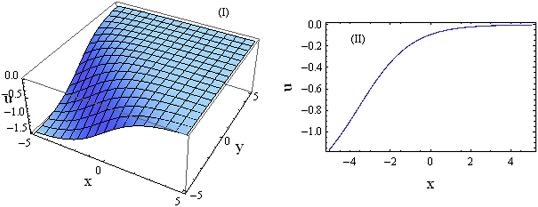
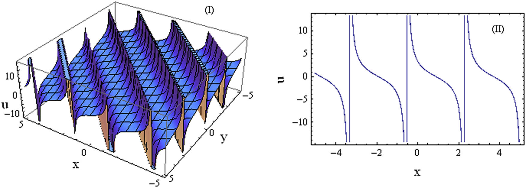
This section presented the physical interpretation of various soliton solutions of the YTSF equation, which were obtained by the proposed analytical method. For selected parameter values, these solutions were illustrated using 3D and 2D graphical representations, highlighting their spatial and temporal structures. The final forms of the YTSF solutions were derived by integrating the analytical expressions, providing a comprehensive view of the solitary wave profiles and their dynamical characteristics
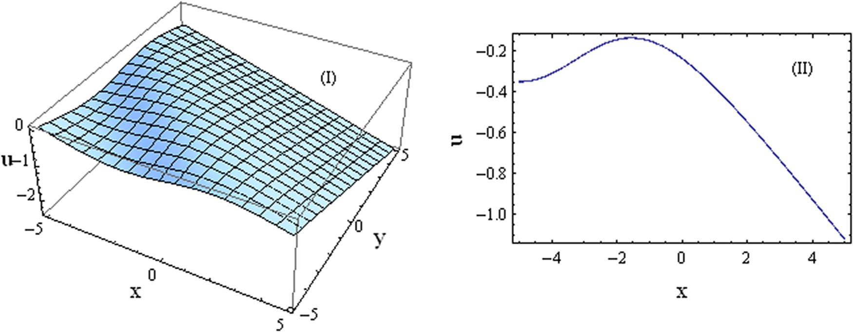
3D and 2D plots of the solution based on

3D and 2D plots of the solution based on
3D and 2D plots of the solution based on
3D and 2D plots of the solution based on
The YTSF equation yields a rich array of solutions that model various coherent wave structures in nonlinear media. Among these are kink and antikink solitons, which describe abrupt, front-like interfaces between two separate equilibrium states, analogous to phenomena like internal tidal bores in oceanography, switching fronts in fiber optics, or transition layers in plasmas. The equation also generates periodic solutions, which represent stable, oscillatory wave trains resulting from the balance of dispersion and nonlinearity. These solutions are comparable to familiar wave packets in internal waves, oscillations in plasma, and pulse trains in optical systems. This diversity of solutions demonstrates the YTSF equation’s capacity to accurately represent a wide spectrum of nonlinear wave behaviors in different dispersive media.
6 Comparative analysis
Recent research has explored exact solutions to higher-dimensional YTSF type equation, focusing on the dynamics and interactions of solitons. A shared methodological foundation, Hirota’s bilinear method, is prevalent across these studies; however, the specific types and scope of solutions investigated show considerable diversity. Alternatively, this research employs a powerful method to derive exact soliton solutions for the YTSF equation, encompassing kink, antikink, periodic, and isolated types. A thorough bifurcation analysis is conducted to identify critical parameter thresholds and characterize transitions into oscillatory or chaotic regimes. The study’s use of 2D and 3D visualizations provides a more comprehensive and predictive characterization of solution dynamics compared to prior work. Table 1 presents a comparative overview of these findings.
Comparative summary of recent studies on YTSF equation
| References | Solution types | Method(s) | Main contribution |
|---|---|---|---|
| Ma et al. [15] |
|
Hirota bilinear method | Explicit
|
| Hu et al. [16] | Kink multisolitons | Hirota method, symbolic computation | First report of kink-type soliton structures in YTSF framework |
| Guo et al. [13] generalized | Abundant solution families | Extended bilinear transformation | Dynamics of generalized YTSF with broad solution structures |
| Huang et al. [12] | Lump, soliton,
|
Bilinear method, spectral analysis | Combination of lump–soliton interactions with integrability verified via LSP |
| Present study | kink, antikink, periodic soliton and bifurcation analysis |
|
Novel exact soliton solutions and bifurcation-based nonlinear wave dynamics |
7 Conclusions
This study employed the powerful
Acknowledgments
The researchers would like to thank the Deanship of Graduate Studies and Scientific Research at the Qassim University for financial support (QU-APC-2025).
-
Funding information: The researchers would like to thank theDeanship of Graduate Studies and Scientific Research at the Qassim University for financial support (QU-APC-2025).
-
Author contributions: R.M., A.A., and A.I.A.S., wrote the main manuscript text, and S.M.B., M.N.H., and M.M.M. prepared figures and supervised this research. All authors have accepted responsibility for the entire content of this manuscript and approved its submission.
-
Conflict of interest: The authors state no conflict of interest.
-
Data availability statement: All data generated or analysed during this study are included in this published article.
References
[1] Hossain MN, Miah MM, Alosaimi M, Alsharif F, Kanan M. Exploring novel soliton solutions to the time-fractional coupled Drinfelad-Sokolov-Wilson equation in industrial engineering using two efficient techniques. Fract Fract. 2024;8:352. 10.3390/fractalfract8060352Suche in Google Scholar
[2] Alharbi A, Almatrafi M. Riccati-Bernoulli sub-ODE approach on the partial differential equations and applications. Int J Math Comput Sci. 2020;15(1):367–88. Suche in Google Scholar
[3] Hamali W, Alghamdi AA. Exact solutions to the fractional nonlinear phenomena in fluid dynamics via the Riccati-Bernoulli sub-ODE method. AIMS Math. 2024;9(11):31142–62. 10.3934/math.20241501Suche in Google Scholar
[4] Asghar U, Asjad MI, Hamed YS, Akgul A, Hassani MK. New exact soliton wave solutions appear in optical fibers with Sardar sub equation and new auxiliary equation techniques. Scientif Rep. 2025;15(1):4396. 10.1038/s41598-024-84651-2Suche in Google Scholar PubMed PubMed Central
[5] Muhammad T, Hamoud AA, Emadifar H, Hamasalh FK, Azizi H, Khademi M. Traveling wave solutions to the Boussinesq equation via Sardar sub-equation technique. AIMS Math. 2022;7(6):11134–49. 10.3934/math.2022623Suche in Google Scholar
[6] Ceesay B, Baber MZ, Ahmed N, Jawaz M, Maciiias-Diiiaz JE, Gallegos A. Harvesting mixed, homoclinic breather, M-shaped, and other wave profiles of the Heisenberg Ferromagnet-type Akbota equation. Europ J Pure Appl Math. 2025;18(2):5851. 10.29020/nybg.ejpam.v18i2.5851Suche in Google Scholar
[7] Khan MI, Farooq A, Nisar KS, Shah NA. Unveiling new exact solutions of the unstable nonlinear Schrödinger equation using the improved modified Sardar sub-equation method. Results Phys. 2024;59:107593. 10.1016/j.rinp.2024.107593Suche in Google Scholar
[8] Yusuf A, Alshomrani AS, Sulaiman TA, Isah I, Baleanu D. Extended classical optical solitons to a nonlinear Schrodinger equation expressing the resonant nonlinear light propagation through isolated flaws in optical waveguides. Opt Quant Elect. 2022;54(12):853. 10.1007/s11082-022-04268-5Suche in Google Scholar
[9] Hossain MD, Boulaaras SM, Saeed AM, Gissy H, Hossain MN, Miah MM. New investigation on soliton solutions of two nonlinear PDEs in mathematical physics with a dynamical property: Bifurcation analysis. Open Phys. 2025;23(1):20250155. 10.1515/phys-2025-0155Suche in Google Scholar
[10] Du Y, Pang J. Localised waves and dynamical behaviours of analytical solutions to (3+1)-dimensional YTSF model in mathematical physics. Pramana J Phys. 2025;99:49. 10.1007/s12043-025-02902-xSuche in Google Scholar
[11] Tan X, Li X. High-order solitons and hybrid behavior of (3+1)-dimensional potential Yu-Toda-Sasa-Fukuyama equation with variable coefficients. J Appl Math Phys. 2024;12:2738–63. 10.4236/jamp.2024.128164Suche in Google Scholar
[12] Huang L, Manafian J, Singh G, Nisar KS, Nasution MKM. New lump and interaction soliton, N-soliton solutions and the LSP for the (3 + 1)-dimensional potential-YTSF-like equation. Results Phys. 2021;29:104713. 10.1016/j.rinp.2021.104713Suche in Google Scholar
[13] Guo HD, Xia TC, Hu BB. Dynamics of abundant solutions to the (3+1)-dimensional generalized Yu-Toda-Sasa-Fukuyama equation. Appl Math Lett. 2020;105:106301. 10.1016/j.aml.2020.106301Suche in Google Scholar
[14] Zhao D, Zhaqilao. The abundant mixed solutions of (2+1)-dimensional potential Yu-Toda-Sasa-Fukuyama equation. Nonlinear Dyn. 2021;103:1055–70. 10.1007/s11071-020-06110-7Suche in Google Scholar
[15] Ma H, Cheng Q, Deng A. N-soliton solutions and localized wave interaction solutions of a (3+1)-dimensional potential-Yu-Toda-Sasa-Fukuyamaf equation. Modern Phys Lett B. 2021;35(10):2150277. 10.1142/S0217984921502778Suche in Google Scholar
[16] Hu Y, Chen H, Dai Z. New kink multi-soliton solutions for the (3+1)-dimensional potential-Yu-Toda-Sasa-Fukuyama equation. Appl Math Comput. 2014;234:548–56. 10.1016/j.amc.2014.02.044Suche in Google Scholar
[17] Hassan S, Abdelrahman MA. A Riccati-Bernoulli sub-ODE method for some nonlinear evolution equations. Int J Nonl Sci Numer Simulat. 2019;20(3–4):303–13. 10.1515/ijnsns-2018-0045Suche in Google Scholar
[18] Hossain MN, El Rashidy K, Alsharif F, Kanan M, Maaa WX, Miah MM. New optical soliton solutions to the Biswas-Milovic equations with power law and parabolic law nonlinearity using the Sardar sub-equation method. Opt Quant Electron. 2024;56:1163. 10.1007/s11082-024-07073-4Suche in Google Scholar
[19] Ceesay B, Baber MZ, Ahmed N, Yasin MW, Mohammed WW. Breather, lump and other wave profiles for the nonlinear Rosenau equation arising in physical systems. Scientif Reports. 2025;15:3067. 10.1038/s41598-024-82678-zSuche in Google Scholar PubMed PubMed Central
[20] Hossain MN, Miah MM, Abbas MS, El-Rashidy K, Borhan JRM, Kanan M. An analytical study of the Mikhailov-Novikov-Wang equation with stability and modulation instability analysis in industrial engineering via multiple methods. Symmetry. 2024;16:879. 10.3390/sym16070879Suche in Google Scholar
[21] Ananna SN, An T, Asaduzzaman M, Rana MS. Sine-Gordon expansion method to construct the solitary wave solutions of a family of 3D fractional WBBM equations. Results Phys. 2022;40:105845. 10.1016/j.rinp.2022.105845Suche in Google Scholar
[22] Shakeel M, Shah NA, Chung JD. Application of modified exp-function method for strain wave equation for finding analytical solutions. Ain Shams Eng J. 2022;14:101883. 10.1016/j.asej.2022.101883Suche in Google Scholar
[23] Ahmad S, Saifullah S, Khan A, Inc M. New local and nonlocal soliton solutions of a nonlocal reverse space-time mKdV equation using improved Hirota bilinear method. Phys Lett A. 2022;450:128393. 10.1016/j.physleta.2022.128393Suche in Google Scholar
[24] Manafian J, Lakestani M, Bekir A. Comparison between the generalized tanh-coth and the (G’/G)-expansion methods for solving NPDEs and NODEs. Pramana. 2016;87(6):1–14. 10.1007/s12043-016-1292-9Suche in Google Scholar
[25] Malik S, Hashemi MS, Kumar S, Rezazadeh H, Mahmoud W, Osman M. Application of new Kudryashov method to various nonlinear partial differential equations. Opt Quantum Electron. 2023;55(1):8. 10.1007/s11082-022-04261-ySuche in Google Scholar
[26] Hosseini K, Mayeli P, Ansari R. Modified Kudryashov method for solving the conformable time-fractional Klein-Gordon equations with quadratic and cubic nonlinearities. Optik. 2017;130:737–42. 10.1016/j.ijleo.2016.10.136Suche in Google Scholar
[27] Ashraf F, Ashraf R, Akgül A. Traveling waves solutions of Hirota-Ramani equation by modified extended direct algebraic method and new extended direct algebraic method. Int J Modern Phys B. 2024;38(24):2450329. 10.1142/S0217979224503296Suche in Google Scholar
[28] Khalique CM, Abdallah SA. Coupled Burgers equations governing polydispersive sedimentation; a Lie symmetry approach. Results Phys. 2020;16:102967. 10.1016/j.rinp.2020.102967Suche in Google Scholar
[29] Ullah MS, Seadawy AR, Ali MZ. Optical soliton solutions to the Fokas-Lenells model applying the varphi 6-model expansion approach. Opt Quantum Electron. 2023;55(6):495. 10.1007/s11082-023-04771-3Suche in Google Scholar
[30] Kurt A, Tasbozan O, Baleanu D. New solutions for conformable fractional Nizhnik-Novikov-Veselov system via (G′∕G,1∕G) expansion method and homotopy analysis methods. Opt Quant Electron. 2017;49:1–16. 10.1007/s11082-017-1163-8Suche in Google Scholar
[31] Yokuş A, Durur H. Complex hyperbolic traveling wave solutions of Kuramoto-Sivashinsky equation using (1∕G′) expansion method for nonlinear dynamic theory. Balıkesir Üniversitesi Fen Bilimleri EnstitüsüDergisi. 2019;21(2):590–9. 10.25092/baunfbed.631193Suche in Google Scholar
[32] Hossain MN, Alsharif F, Miah MM, Kanan M. Abundant new optical soliton solutions to the Biswas-Milovic equation with sensitivity analysis for optimization. Mathematics. 2024;12:1585. 10.3390/math12101585Suche in Google Scholar
[33] Hussain A, Chahlaoui Y, Zaman F, Parveen T, Hassan AM. The Jacobi elliptic function method and its application for the stochastic NNV system. Alexandr Eng J. 2023;81:347–59. 10.1016/j.aej.2023.09.017Suche in Google Scholar
[34] Akter J, Akbar MA. Exact solutions to the Benney-Luke equation and the Phi-4 equations by using modified simple equation method. Results Phys. 2015;5:125–30. 10.1016/j.rinp.2015.01.008Suche in Google Scholar
[35] Elsherbeny AM, Murad MAS, Arnous AH, Biswas A, Moraru L, Yildirim Y. Quiescent optical soliton perturbation for Fokas-Lenells equation with nonlinear chromatic dispersion and generalized quadratic-cubic form of self-phase modulation structure. Contemporary Math. 2025:2308–38. 10.37256/cm.6220256359Suche in Google Scholar
[36] Akram G, Arshed S, Sadaf M, Khan A. Extraction of new soliton solutions of (3+1)-dimensional nonlinear extended quantum Zakharov-Kuznetsov equation via generalized exponential rational function method and (G′∕G,1∕G) expansion method. Opt Quant Electron. 2024;56(5):829. 10.1007/s11082-024-06662-7Suche in Google Scholar
[37] Hossain AKS, Akter H, Akbar MA. Soliton solutions of DSW and Burgers equations by generalized (G′∕G)-expansion method. Opt Quant Electron. 2024;56(4):653. 10.1007/s11082-024-06319-5Suche in Google Scholar
[38] Hong B, Chen W, Zhang S, Xub J. The (G′∕(G′.G.A))-expansion method for two types of nonlinear Schrödinger equations. J Math Phys. 2019;31(5):1155–6. Suche in Google Scholar
[39] Tripathy A, Sahoo S. Exact solutions for the ion sound Langmuir wave model by using two novel analytical methods. Results Phys. 2020;19:103494. 10.1016/j.rinp.2020.103494Suche in Google Scholar
[40] Ahmad I, Jalil A, Ullah A, Ahmad S, DelaSen M. Some new exact solutions of (4+1)-dimensional Davey-Stewartson-Kadomtsev-Petviashvili equation. Results Phys. 2023;45:106240. 10.1016/j.rinp.2023.106240Suche in Google Scholar
[41] Mia R, Miah MM, Osman M. A new implementation of a novel analytical method for finding the analytical solutions of the (2+1)-dimensional KP-BBM equation. Heliyon. 2023;9(5):e15690. 10.1016/j.heliyon.2023.e15690Suche in Google Scholar PubMed PubMed Central
[42] Mia R, Paul AK. New exact solutions to the generalized shallow water wave equation. Modern Phys Lett B. 2024;38(31):2450301. 10.1142/S0217984924503019Suche in Google Scholar
[43] Hossain MN, Miah MM, Duraihem FZ, Rehman S, Maaa WX. Chaotic behavior, bifurcations, sensitivity analysis, and novel optical soliton solutions to the Hamiltonian amplitude equation in optical physics. Phys Scr. 2024;99:075231. 10.1088/1402-4896/ad52fdSuche in Google Scholar
[44] Taskeen A, Ahmed MO, Baber MZ, Ceesay B, Ahamed N. Bifurcation, chaotic, sensitivity analysis, and optical soliton profiles for the spin Hirota-Maxwell-Bloch equation in an Erbium-Doped fiber. Adv Math Phys. 2025;2025:7157902. 10.1155/admp/7157902Suche in Google Scholar
[45] Wang KJ, Zhu HW, Li S, Shi F, Li G, Liu XL. Bifurcation analysis, chaotic behaviors, variational principle, Hamiltonian and diverse optical solitons of the fractional complex Ginzburg-Landau model. Int J Theoret Phys. 2025;64(5):1–20. 10.1007/s10773-025-05977-9Suche in Google Scholar
[46] Hossain MN, Rasid MM, Abouelfarag I, El-Rashidy K, Miah MM, Kanan M. A new investigation of the extended Sakovich equation for abundant soliton solution in industrial engineering via two efficient techniques. Open Phys. 2024;22(1):20240096. 10.1515/phys-2024-0096Suche in Google Scholar
© 2025 the author(s), published by De Gruyter
This work is licensed under the Creative Commons Attribution 4.0 International License.
Artikel in diesem Heft
- Research Articles
- Single-step fabrication of Ag2S/poly-2-mercaptoaniline nanoribbon photocathodes for green hydrogen generation from artificial and natural red-sea water
- Abundant new interaction solutions and nonlinear dynamics for the (3+1)-dimensional Hirota–Satsuma–Ito-like equation
- A novel gold and SiO2 material based planar 5-element high HPBW end-fire antenna array for 300 GHz applications
- Explicit exact solutions and bifurcation analysis for the mZK equation with truncated M-fractional derivatives utilizing two reliable methods
- Optical and laser damage resistance: Role of periodic cylindrical surfaces
- Numerical study of flow and heat transfer in the air-side metal foam partially filled channels of panel-type radiator under forced convection
- Water-based hybrid nanofluid flow containing CNT nanoparticles over an extending surface with velocity slips, thermal convective, and zero-mass flux conditions
- Dynamical wave structures for some diffusion--reaction equations with quadratic and quartic nonlinearities
- Solving an isotropic grey matter tumour model via a heat transfer equation
- Study on the penetration protection of a fiber-reinforced composite structure with CNTs/GFP clip STF/3DKevlar
- Influence of Hall current and acoustic pressure on nanostructured DPL thermoelastic plates under ramp heating in a double-temperature model
- Applications of the Belousov–Zhabotinsky reaction–diffusion system: Analytical and numerical approaches
- AC electroosmotic flow of Maxwell fluid in a pH-regulated parallel-plate silica nanochannel
- Interpreting optical effects with relativistic transformations adopting one-way synchronization to conserve simultaneity and space–time continuity
- Modeling and analysis of quantum communication channel in airborne platforms with boundary layer effects
- Theoretical and numerical investigation of a memristor system with a piecewise memductance under fractal–fractional derivatives
- Tuning the structure and electro-optical properties of α-Cr2O3 films by heat treatment/La doping for optoelectronic applications
- High-speed multi-spectral explosion temperature measurement using golden-section accelerated Pearson correlation algorithm
- Dynamic behavior and modulation instability of the generalized coupled fractional nonlinear Helmholtz equation with cubic–quintic term
- Study on the duration of laser-induced air plasma flash near thin film surface
- Exploring the dynamics of fractional-order nonlinear dispersive wave system through homotopy technique
- The mechanism of carbon monoxide fluorescence inside a femtosecond laser-induced plasma
- Numerical solution of a nonconstant coefficient advection diffusion equation in an irregular domain and analyses of numerical dispersion and dissipation
- Numerical examination of the chemically reactive MHD flow of hybrid nanofluids over a two-dimensional stretching surface with the Cattaneo–Christov model and slip conditions
- Impacts of sinusoidal heat flux and embraced heated rectangular cavity on natural convection within a square enclosure partially filled with porous medium and Casson-hybrid nanofluid
- Stability analysis of unsteady ternary nanofluid flow past a stretching/shrinking wedge
- Solitonic wave solutions of a Hamiltonian nonlinear atom chain model through the Hirota bilinear transformation method
- Bilinear form and soltion solutions for (3+1)-dimensional negative-order KdV-CBS equation
- Solitary chirp pulses and soliton control for variable coefficients cubic–quintic nonlinear Schrödinger equation in nonuniform management system
- Influence of decaying heat source and temperature-dependent thermal conductivity on photo-hydro-elasto semiconductor media
- Dissipative disorder optimization in the radiative thin film flow of partially ionized non-Newtonian hybrid nanofluid with second-order slip condition
- Bifurcation, chaotic behavior, and traveling wave solutions for the fractional (4+1)-dimensional Davey–Stewartson–Kadomtsev–Petviashvili model
- New investigation on soliton solutions of two nonlinear PDEs in mathematical physics with a dynamical property: Bifurcation analysis
- Mathematical analysis of nanoparticle type and volume fraction on heat transfer efficiency of nanofluids
- Creation of single-wing Lorenz-like attractors via a ten-ninths-degree term
- Optical soliton solutions, bifurcation analysis, chaotic behaviors of nonlinear Schrödinger equation and modulation instability in optical fiber
- Chaotic dynamics and some solutions for the (n + 1)-dimensional modified Zakharov–Kuznetsov equation in plasma physics
- Fractal formation and chaotic soliton phenomena in nonlinear conformable Heisenberg ferromagnetic spin chain equation
- Single-step fabrication of Mn(iv) oxide-Mn(ii) sulfide/poly-2-mercaptoaniline porous network nanocomposite for pseudo-supercapacitors and charge storage
- Novel constructed dynamical analytical solutions and conserved quantities of the new (2+1)-dimensional KdV model describing acoustic wave propagation
- Tavis–Cummings model in the presence of a deformed field and time-dependent coupling
- Spinning dynamics of stress-dependent viscosity of generalized Cross-nonlinear materials affected by gravitationally swirling disk
- Design and prediction of high optical density photovoltaic polymers using machine learning-DFT studies
- Robust control and preservation of quantum steering, nonlocality, and coherence in open atomic systems
- Coating thickness and process efficiency of reverse roll coating using a magnetized hybrid nanomaterial flow
- Dynamic analysis, circuit realization, and its synchronization of a new chaotic hyperjerk system
- Decoherence of steerability and coherence dynamics induced by nonlinear qubit–cavity interactions
- Finite element analysis of turbulent thermal enhancement in grooved channels with flat- and plus-shaped fins
- Modulational instability and associated ion-acoustic modulated envelope solitons in a quantum plasma having ion beams
- Statistical inference of constant-stress partially accelerated life tests under type II generalized hybrid censored data from Burr III distribution
- On solutions of the Dirac equation for 1D hydrogenic atoms or ions
- Entropy optimization for chemically reactive magnetized unsteady thin film hybrid nanofluid flow on inclined surface subject to nonlinear mixed convection and variable temperature
- Stability analysis, circuit simulation, and color image encryption of a novel four-dimensional hyperchaotic model with hidden and self-excited attractors
- A high-accuracy exponential time integration scheme for the Darcy–Forchheimer Williamson fluid flow with temperature-dependent conductivity
- Novel analysis of fractional regularized long-wave equation in plasma dynamics
- Development of a photoelectrode based on a bismuth(iii) oxyiodide/intercalated iodide-poly(1H-pyrrole) rough spherical nanocomposite for green hydrogen generation
- Investigation of solar radiation effects on the energy performance of the (Al2O3–CuO–Cu)/H2O ternary nanofluidic system through a convectively heated cylinder
- Quantum resources for a system of two atoms interacting with a deformed field in the presence of intensity-dependent coupling
- Studying bifurcations and chaotic dynamics in the generalized hyperelastic-rod wave equation through Hamiltonian mechanics
- A new numerical technique for the solution of time-fractional nonlinear Klein–Gordon equation involving Atangana–Baleanu derivative using cubic B-spline functions
- Interaction solutions of high-order breathers and lumps for a (3+1)-dimensional conformable fractional potential-YTSF-like model
- Hydraulic fracturing radioactive source tracing technology based on hydraulic fracturing tracing mechanics model
- Numerical solution and stability analysis of non-Newtonian hybrid nanofluid flow subject to exponential heat source/sink over a Riga sheet
- Numerical investigation of mixed convection and viscous dissipation in couple stress nanofluid flow: A merged Adomian decomposition method and Mohand transform
- Effectual quintic B-spline functions for solving the time fractional coupled Boussinesq–Burgers equation arising in shallow water waves
- Analysis of MHD hybrid nanofluid flow over cone and wedge with exponential and thermal heat source and activation energy
- Solitons and travelling waves structure for M-fractional Kairat-II equation using three explicit methods
- Impact of nanoparticle shapes on the heat transfer properties of Cu and CuO nanofluids flowing over a stretching surface with slip effects: A computational study
- Computational simulation of heat transfer and nanofluid flow for two-sided lid-driven square cavity under the influence of magnetic field
- Irreversibility analysis of a bioconvective two-phase nanofluid in a Maxwell (non-Newtonian) flow induced by a rotating disk with thermal radiation
- Hydrodynamic and sensitivity analysis of a polymeric calendering process for non-Newtonian fluids with temperature-dependent viscosity
- Exploring the peakon solitons molecules and solitary wave structure to the nonlinear damped Kortewege–de Vries equation through efficient technique
- Modeling and heat transfer analysis of magnetized hybrid micropolar blood-based nanofluid flow in Darcy–Forchheimer porous stenosis narrow arteries
- Activation energy and cross-diffusion effects on 3D rotating nanofluid flow in a Darcy–Forchheimer porous medium with radiation and convective heating
- Insights into chemical reactions occurring in generalized nanomaterials due to spinning surface with melting constraints
- Influence of a magnetic field on double-porosity photo-thermoelastic materials under Lord–Shulman theory
- Soliton-like solutions for a nonlinear doubly dispersive equation in an elastic Murnaghan's rod via Hirota's bilinear method
- Analytical and numerical investigation of exact wave patterns and chaotic dynamics in the extended improved Boussinesq equation
- Nonclassical correlation dynamics of Heisenberg XYZ states with (x, y)-spin--orbit interaction, x-magnetic field, and intrinsic decoherence effects
- Exact traveling wave and soliton solutions for chemotaxis model and (3+1)-dimensional Boiti–Leon–Manna–Pempinelli equation
- Unveiling the transformative role of samarium in ZnO: Exploring structural and optical modifications for advanced functional applications
- On the derivation of solitary wave solutions for the time-fractional Rosenau equation through two analytical techniques
- Analyzing the role of length and radius of MWCNTs in a nanofluid flow influenced by variable thermal conductivity and viscosity considering Marangoni convection
- Advanced mathematical analysis of heat and mass transfer in oscillatory micropolar bio-nanofluid flows via peristaltic waves and electroosmotic effects
- Exact bound state solutions of the radial Schrödinger equation for the Coulomb potential by conformable Nikiforov–Uvarov approach
- Some anisotropic and perfect fluid plane symmetric solutions of Einstein's field equations using killing symmetries
- Nonlinear dynamics of the dissipative ion-acoustic solitary waves in anisotropic rotating magnetoplasmas
- Curves in multiplicative equiaffine plane
- Exact solution of the three-dimensional (3D) Z2 lattice gauge theory
- Propagation properties of Airyprime pulses in relaxing nonlinear media
- Symbolic computation: Analytical solutions and dynamics of a shallow water wave equation in coastal engineering
- Wave propagation in nonlocal piezo-photo-hygrothermoelastic semiconductors subjected to heat and moisture flux
- Comparative reaction dynamics in rotating nanofluid systems: Quartic and cubic kinetics under MHD influence
- Laplace transform technique and probabilistic analysis-based hypothesis testing in medical and engineering applications
- Physical properties of ternary chloro-perovskites KTCl3 (T = Ge, Al) for optoelectronic applications
- Gravitational length stretching: Curvature-induced modulation of quantum probability densities
- The search for the cosmological cold dark matter axion – A new refined narrow mass window and detection scheme
- A comparative study of quantum resources in bipartite Lipkin–Meshkov–Glick model under DM interaction and Zeeman splitting
- PbO-doped K2O–BaO–Al2O3–B2O3–TeO2-glasses: Mechanical and shielding efficacy
- Nanospherical arsenic(iii) oxoiodide/iodide-intercalated poly(N-methylpyrrole) composite synthesis for broad-spectrum optical detection
- Sine power Burr X distribution with estimation and applications in physics and other fields
- Numerical modeling of enhanced reactive oxygen plasma in pulsed laser deposition of metal oxide thin films
- Dynamical analyses and dispersive soliton solutions to the nonlinear fractional model in stratified fluids
- Computation of exact analytical soliton solutions and their dynamics in advanced optical system
- An innovative approximation concerning the diffusion and electrical conductivity tensor at critical altitudes within the F-region of ionospheric plasma at low latitudes
- An analytical investigation to the (3+1)-dimensional Yu–Toda–Sassa–Fukuyama equation with dynamical analysis: Bifurcation
- Swirling-annular-flow-induced instability of a micro shell considering Knudsen number and viscosity effects
- Review Article
- Examination of the gamma radiation shielding properties of different clay and sand materials in the Adrar region
- Erratum
- Erratum to “On Soliton structures in optical fiber communications with Kundu–Mukherjee–Naskar model (Open Physics 2021;19:679–682)”
- Special Issue on Fundamental Physics from Atoms to Cosmos - Part II
- Possible explanation for the neutron lifetime puzzle
- Special Issue on Nanomaterial utilization and structural optimization - Part III
- Numerical investigation on fluid-thermal-electric performance of a thermoelectric-integrated helically coiled tube heat exchanger for coal mine air cooling
- Special Issue on Nonlinear Dynamics and Chaos in Physical Systems
- Analysis of the fractional relativistic isothermal gas sphere with application to neutron stars
- Abundant wave symmetries in the (3+1)-dimensional Chafee–Infante equation through the Hirota bilinear transformation technique
- Successive midpoint method for fractional differential equations with nonlocal kernels: Error analysis, stability, and applications
- Novel exact solitons to the fractional modified mixed-Korteweg--de Vries model with a stability analysis