
Dynamical analyses and dispersive soliton solutions to the nonlinear fractional model in stratified fluids
-
Muhammad Bilal
 und
Mustafa Inc
und
Mustafa Inc

Abstract
This study explores the bifurcation analysis, sensitivity analysis (SA), stability analysis, and exact solitonic wave profiles for the time-fractional Benjamin–Ono (BO) equation, which models internal waves in stratified fluids, especially where dispersive effects play a significant role. These solutions are crucial for understanding ocean engineering and mathematical physics phenomena. The BO equation simulates deep-water waves, making it essential for ocean engineering applications. We employ some diverse strategies such as the new extended direct algebraic method, generalized Arnous method, and ansatz method to extract novel dispersive wave solutions. These solutions exhibit diverse shapes, such as hyperbolic, singular periodic, exponential, rational function solutions and solitary waves including dark, singular, bright, combo, and complex solutions. Our main goal is to analyze the dynamic characteristics of the model by conducting bifurcation and SA and identify the corresponding Hamiltonian function. To ensure validity, we also conduct stability analysis using linear stability theory and outline constraint conditions. Furthermore, the bifurcation of phase portraits of ordinary differential equations corresponding to partial differential equations under investigation is also analyzed. We also demonstrate the fractional behavior of our results through visualizations (2D, 3D, contour, and density plots) by selecting suitable parametric values. Our reported results are verified using Mathematica to guarantee accuracy and validity. A detailed comparison with existing results highlights the novelty of our findings. This research contributes significantly to understand wave dynamics in nonlinear phenomena and the unique outcomes explored in this research will play a significant role in the forthcoming investigation of nonlinear problems. Moreover, the novelty of this study lies in the fact that the proposed model has not been previously explored using the aforementioned advanced methods and comprehensive dynamical analyses. This study pioneers the exploration of the fractional BO equation, yielding unique analytical results. Our techniques efficiently identify accurate solitary pulse solutions to nonlinear dynamical models with fractional parameters, making them highly successful in modeling deep-water internal waves. Our computational analytical tools are also straightforward, transparent, and reliable, reducing complexity while widening applicability. The acquired solutions are expected to have a profound impact on the study of wave propagation and related fields, offering new insights and perspectives that can inform future research and applications.
1 Introduction
In this modern technological era, engineers and scholars have been increasingly interested in obtaining exact solutions to nonlinear partial differential equations (NLPDEs) using computational tools. These tools simplify complex mathematical calculations and play a key role in describing various physical systems and dynamic processes in fields such as plasma physics, fluid mechanics, hydrodynamics, quantum electronics, mathematical biology, ocean engineering, geochemistry, optical fibers, physics, and so on [1–5]. The intrinsic nonlinearity of natural phenomena has long fascinated scientists, who recognize it as a crucial element in unraveling the complexities of the universe. A plethora of physical phenomena in the universe, characterized by enigmatic behaviors, inherently involve nonlinear and dispersive components. The NLPDEs, effectively model nonlinear physical phenomena like wave propagation and instability. Mathematicians and researchers widely use these equations to study complex nonlinear wave dynamics. A dynamical system is a mathematical framework used to describe how a system evolves over time. The system’s behavior is governed by differential equations, which capture its time-dependent dynamics. Dynamical systems are employed across various fields to analyze the behavior of complex systems. These fields include mathematical physics, economics, nonlinear optics, engineering, and many others.
1.1 Background and literature review
In recent years, the pursuit of analytical solutions to complex NLPDEs has emerged as a vital and captivating area of research. Notably, in the realm of soliton theory within mathematical physics, the precise solutions of NLPDEs hold paramount significance. NLPDEs serve as the fundamental tool for describing nonlinear phenomena, providing a profound understanding of their fluctuating behaviors and oscillatory mechanisms. The study of nonlinear phenomena has become particularly captivating in modern science. Consequently, there is a growing interest in utilizing efficient computational packages to secure exact solutions, thereby alleviating the complexities of algebraic computations. Various robust, efficient, and reliable analytical methods have been established in the existing literature to explore different types of solutions for nonlinear physical models [6–13].
Fractional differential equations involve derivatives of fractional order, adding complexity to the mathematical models. These equations are prominent in soliton wave theory, presenting challenges in their analysis. However, they offer a more accurate representation of real-world phenomena and find extensive applications across nonlinear sciences. Conformable fractional operators, which maintain traditional calculus properties like Rolle’s theorem and the chain rule, provide a convenient framework for comparison with existing fractional operators [14,15]. Their ease of use makes them a natural choice for practical applications and aids in understanding physical phenomena. These operators have diverse applications in different regions such as nonlinear dynamics, optical fibers, chemistry, laser optics, biology, computing networking, and engineering [16–18]. Their versatility and compatibility with established calculus principles make them valuable tools in different engineering and scientific fields.
1.2 The studied model
The Benjamin–Ono (BO) equation is a significant nonlinear model in mathematics that helps to describe one-dimensional internal waves in deep water. It was derived by two mathematicians named Benjamin [19] and Ono [20]. This partial differential equation (PDE) illustrates how one-dimensional internal waves propagate across a two-layer fluid. It represents the behavior of internal waves existing in the depths of the fluid. This equation, developed by Ono and Benjamin T. Brook, is widely used in fluid dynamics and mathematical physics to study wave interactions, the evolution of wave behaviors, and wave breaking. The BO equation [20], which looks like the Korteweg–de Vries equation, was stated to elucidate internal waves in stratified fluids. It has also been applied to simulate surface wave propagation on a thinly layered structure [21], using a surface acoustic wave delay line to launch the waves. The BO equation plays a crucial role in understanding various phenomena related to internal waves [22]. In the recent past, extensive work has been done on a given model. Li [23] retrieved solutions through the trial equation method. Taghizadeh et al. [24] found exact traveling solutions with the aid of the homogeneous balance method. Kaplan et al. [25] discussed accurate solutions and conservation laws via the
where
1.3 Research aim and gap of the study
In this article, our main aim is to explore time fractional (1+1)-dimensional BO equation analytically to obtain single and combined forms of complex wave solutions of the governing model under specified parametric circumstances by the new extended direct algebraic method (NEDAM), generalized Arnous method (GAM), and ansatz method [28–30], respectively. A comprehensive review of existing literature on the BO equation reveals a significant knowledge gap: the NEDAM, GAM, and ansatz methods have not been previously utilized, and dynamical perspective of sensitivity, bifurcation, and stability analyses remains unexplored. This notable oversight underscores the importance of our research, which aims to bridge this gap by applying these innovative methods to derive novel wave structures and qualitative analyses, thereby enriching our understanding of the BO equation and its dynamics. Our current motivation is on leveraging these advanced methods to systematically investigate different classes of solutions. Furthermore, we have established a framework to efficiently categorize the solutions acquired from these innovative techniques. The methodologies employed in this study offer a significant advantage over existing methods, as they yield additional computable solutions with extra free parameters. The selection of the NEDAM, GAM, and ansatz method over conventional approaches such as the variational iteration method (VIM), Adomian decomposition method (ADM), and Hirota bilinear method (HBM) lacks a comprehensive comparative discussion in many studies. Unlike VIM and ADM, which rely on iterative corrections and series expansions, these algebraic methods offer a more direct route to exact solutions without requiring approximations or decompositions. Compared to HBM, which is limited to integrable equations and requires bilinear transformations, NEDAM, GAM, and the ansatz method apply to a broader class of nonlinear differential equations. Their primary advantage lies in their efficiency and ability to generate closed-form solutions, making them particularly useful for soliton, periodic, and rational wave solutions. However, they are limited by their reliance on correctly assuming the solution structure, a challenge not faced by iterative methods that refine approximations progressively. Additionally, while VIM and ADM provide error estimates and convergence guarantees, these algebraic methods lack inherent mechanisms to assess accuracy or stability. Despite these limitations, their ability to produce exact analytical solutions makes them valuable for exploring the fundamental properties of nonlinear evolution equations, especially in mathematical physics. Notably, many previously obtained solutions in the literature can be derived as special cases using these approaches, and importantly, new solutions are also obtained. The recommended computational methods are characterized by their simplicity, clarity, consistency, and reduced computational complexity, making them widely applicable. Furthermore, these approaches facilitate the discovery of novel results, furnishing a comprehensive framework for systematically organizing and consolidating these findings.
1.4 Structure of the study
The article is organized as follows: Conformable fractional derivative with its features is given in Section 2. Extraction of diverse traveling wave solutions is given in Section 3. In Section 4, we will discuss the sensitivity analysis (SA) of the dynamical model. Section 5 deals with bifurcation analysis. In Section 6, stability analysis is examined. In Section 7, results and discussion are represented. In Section 8, the concluding remarks are revealed.
2 Conformable derivative and its properties
The widespread applications of conformable derivatives highlight the need for more accurate mathematical methods when addressing real-world phenomena. Researchers have been exploring the behavior of nonlinear fractional partial differential equations (FPDEs) using innovative forms of fractional calculus operators like the Riemann–Liouville, Caputo-Fabrizio, and the Beta derivative. These models play a crucial role in engineering and applied sciences, offering solutions to complex problems. This particular class of derivatives offers a potent tool for scholars and practitioners to elucidate and examine a diverse range of physical, biological, and engineering systems. Among these models, the conformable fractional derivative is notable for its proficiency to reveal the core of the basic phenomenon.
Furthermore, if
Lemma 1
If
If
The choice of the conformable derivative over Caputo or Riemann–Liouville derivatives reflects a trade-off between capturing memory effects and ensuring analytical tractability. While Caputo and Riemann–Liouville formulations inherently model memory through non-local integral operators, their complexity often complicates analytical solutions, numerical implementation, and physical interpretation. The conformable derivative, though lacking explicit memory representation, offers a local, Leibniz-like structure that simplifies computations, preserves classical calculus rules, and facilitates explicit solutions – advantages critical for modeling systems where memory effects are secondary to simplicity, interpretability, or real time applicability. This prioritization of tractability makes conformable derivatives pragmatic for applications where approximate or efficient modeling suffices. The conformable derivative is a type of fractional derivative proposed to maintain compatibility with classical calculus, particularly the limit definition. It offers a physically meaningful way to explain memory and hereditary features in intricate systems. Its simplicity and local nature make it suitable for modeling time-dependent processes in physics and engineering problems.
3 Diversity of traveling wave solutions
In this section, we utilize different techniques to earn some soliton solutions of the studied model. Prior to extracting the results we present some characteristics and weakness of the aforementioned mathematical techniques.
The NEDAM is a powerful analytical technique for obtaining exact solutions of nonlinear evolution equations, especially soliton and periodic wave solutions. It extends traditional direct algebraic approaches by incorporating more general ansatz functions and higher-degree polynomials, allowing for a wider variety of solution forms. This method is valued for its systematic structure, applicability to diverse nonlinear PDEs, and ability to generate multiple types of exact solutions, including dark, bright, combine, and rational-type structures. However, it may become computationally intensive for complex equations due to the algebraic system’s size and complexity.
The GAM refines and extends classical ansatz-based techniques by incorporating hyperbolic and trigonometric function expansions to construct more general analytical solutions. It is particularly effective in generating traveling wave solutions and is simpler in structure, often reducing the PDE to an ordinary differential equation via wave transformation before solving. This method is appreciated for its simplicity, versatility, and relatively low computational burden, but it can be limited in scope, often failing to capture more complex or nonstandard wave structures that the extended direct algebraic method can handle.
3.1 Application of NEDAM
The NEDAM generates a wide variety of exact solutions for nonlinear PDEs, offering flexibility and precision. It is applicable to diverse physical problems and reduces computational complexity. However, this technique has a limitation: it is ineffective when the highest derivative terms do not uniformly balance with nonlinear terms. To solve the above system by utilizing NEDAM, we use traveling wave transformation
By applying the balance principle to Eq. (2) and equating the powers of
By substituting Eq. (4) and its derivatives
Family-1.
We construct multiple outcomes to Eq. (1) as follows.
(1) For
The trigonometric solutions
(2) For
The dark solution is as follows:
The singular solution is as follows:
The complex dark-bright solution is as follows:
The mixed singular solution is as follows:
The dark-singular solution is as follows:
(3) For
The periodic solutions are as follows:
Now, the mixed-trigonometric solutions are as follows:
(4) For
The hyperbolic solution is as follows:
The singular solution is as follows:
The different types of complex wave structures are as follows:
(5) For
The periodic wave solutions are as follows:
(6) For
Exact wave solutions are as follows:
(8) For
Combined-hyperbolic solutions are as follows:
(9) For
Rational function solution is as follows:
where
3.2 Application of GAM
The GAM effectively derives exact solutions for nonlinear equations with strong nonlinearity and dispersion. It transforms equations into simpler forms, yielding explicit solutions, and adapts to various nonlinear evolution equations. However, this method has a limitation: it is ineffective when the highest derivative terms do not uniformly balance with nonlinear terms. In this section, we employ the GAM to derive solitary wave solutions to the BO equation. The GAM involves assuming a solution of the form
For
By substituting Eq. (39) into Eq. (2) along with its derivatives
and
According to set-1
At
According to set-2
At
3.3 Ansatz method
To construct the solutions, hyperbolic and exponential ansatz method is used in Sections 3.3.1–3.3.3
3.3.1 Solitary wave solution
For solitary wave solutions, we have
where
Solving the above equations we achieve
Hence, the solitary wave solution is presented as
3.3.2 Dark wave solution
For dark wave solutions, we obtain
where
Solving the above system we achieve
Hence, the dark wave solution is presented as
3.3.3 Exponential solution
For exponential solution, we have
where
Solving the above system we achieve
Hence, the exponential solution is presented as
4 SA
This section explores the SA of the governing model. SA [33,34] of dynamical models offers valuable insights into system behavior, supports model validation and calibration, aids in risk assessment and management, guides optimization and control strategies, and contributes to uncertainty quantification. Our approach investigates the effects of small perturbations in initial conditions on the system’s dynamics. We analyze Eq. (2) and transform it into a dynamical system
where
Graphical visualization of SA for Eq. (51) with initial conditions
Graphical visualization of SA for Eq. (51) with initial conditions
Graphical visualization of SA for Eq. (51) with initial conditions
Graphical visualization of SA for Eq. (51) with initial conditions
5 Bifurcation analysis
The primary objective of bifurcation analysis is to comprehend how the qualitative behavior of a dynamical system evolves as a parameter is varied. A bifurcation occurs when such variations induce substantial changes in the system, giving rise to new dynamic behaviors. As the parameter shifts, equilibrium points, periodic patterns, or other system features may emerge, vanish, or experience changes in stability [35–37]. Using bifurcation theory, we shall analyze Eq. (1) in this section. It is possible to examine governing equation as a planar dynamical system by applying a Galilean transformation.
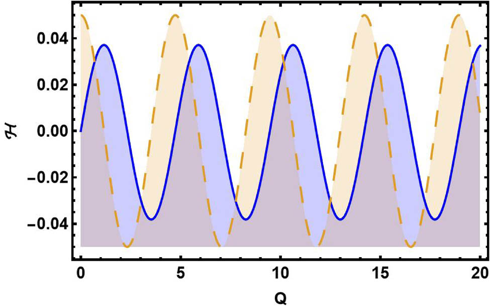
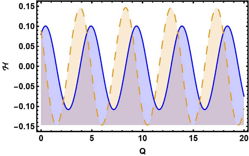
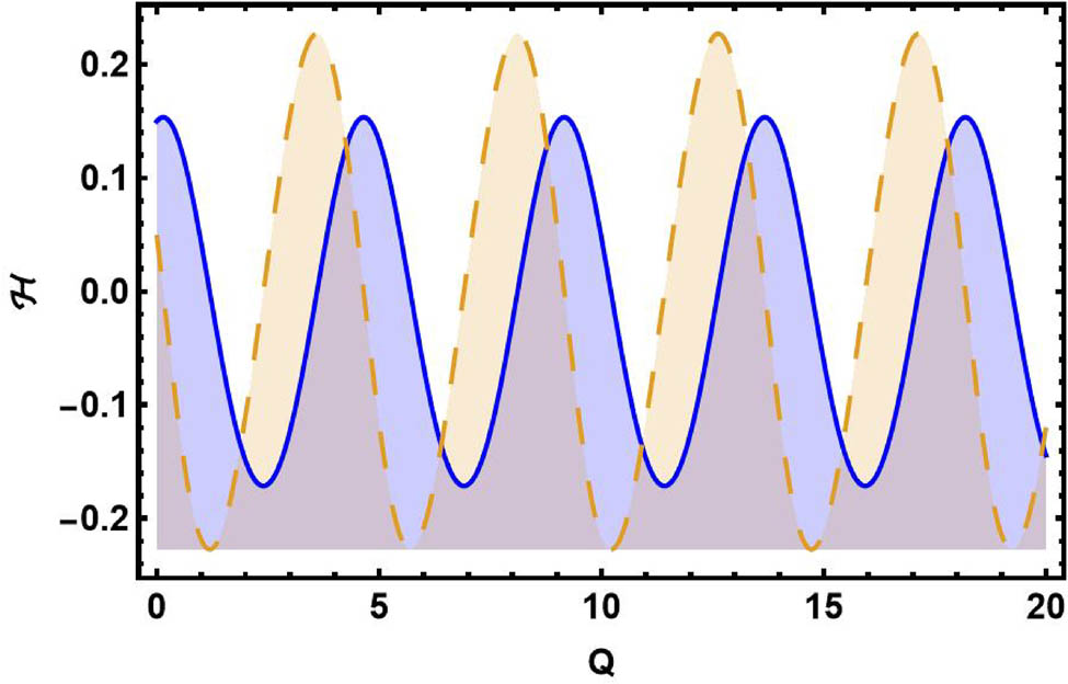
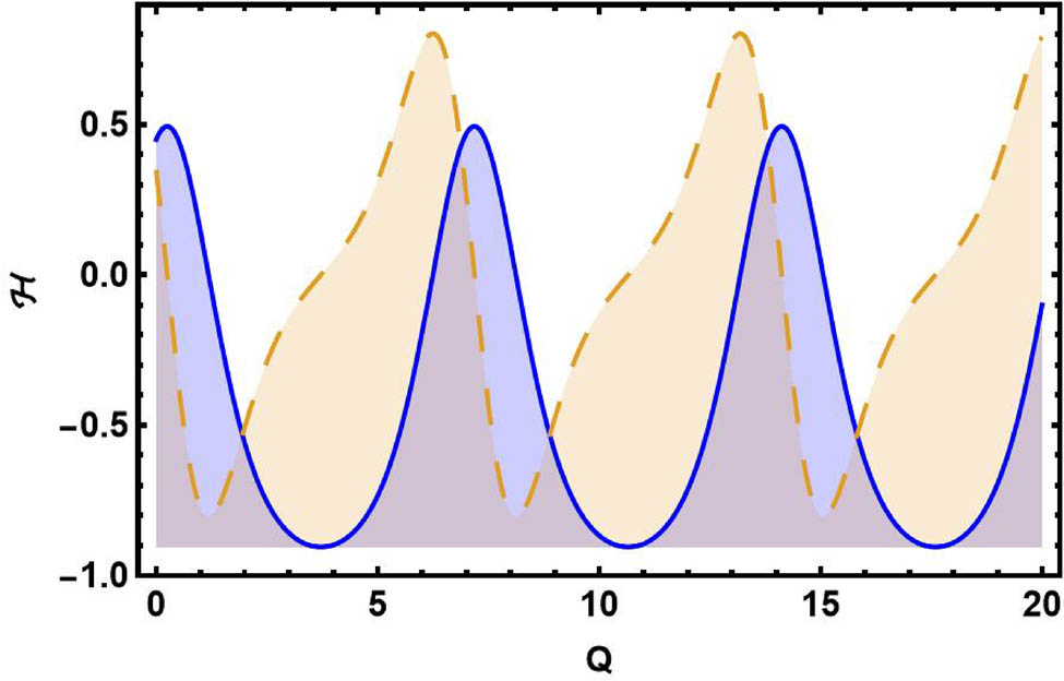
The Hamiltonian function for Eq. (52) is
The Hamiltonian function plays a crucial role in governing the dynamics of a system by representing its total energy, typically comprising kinetic and potential components. In conservative systems, where the Hamiltonian is time-independent, it acts as a conserved quantity, ensuring energy preservation and constraining phase-space trajectories. This conservation property directly influences stability, equilibrium behavior, and integrability, as systems with a well-defined Hamiltonian often exhibit structured dynamics, such as periodic or quasi-periodic motion. Moreover, in canonical Hamiltonian systems, Poisson brackets govern evolution, ensuring symplectic structure preservation and enabling the application of powerful analytical techniques like Liouville’s theorem and integrability analysis. When the Hamiltonian structure is perturbed or non-existent, dissipative effects arise, leading to energy dissipation and potentially chaotic behavior, highlighting its fundamental role in differentiating between stable and non-conservative dynamics. To solve system (52), the system (52) has two equilibrium points, which are listed below:
We know that
If
If
If
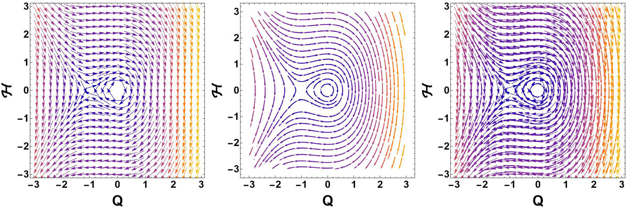
Case-1: When
By picking certain values for the parameters
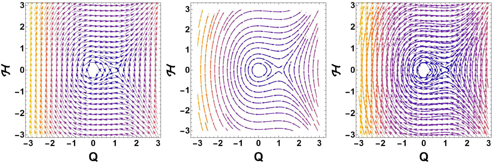
Case-2: When
By setting the parameters
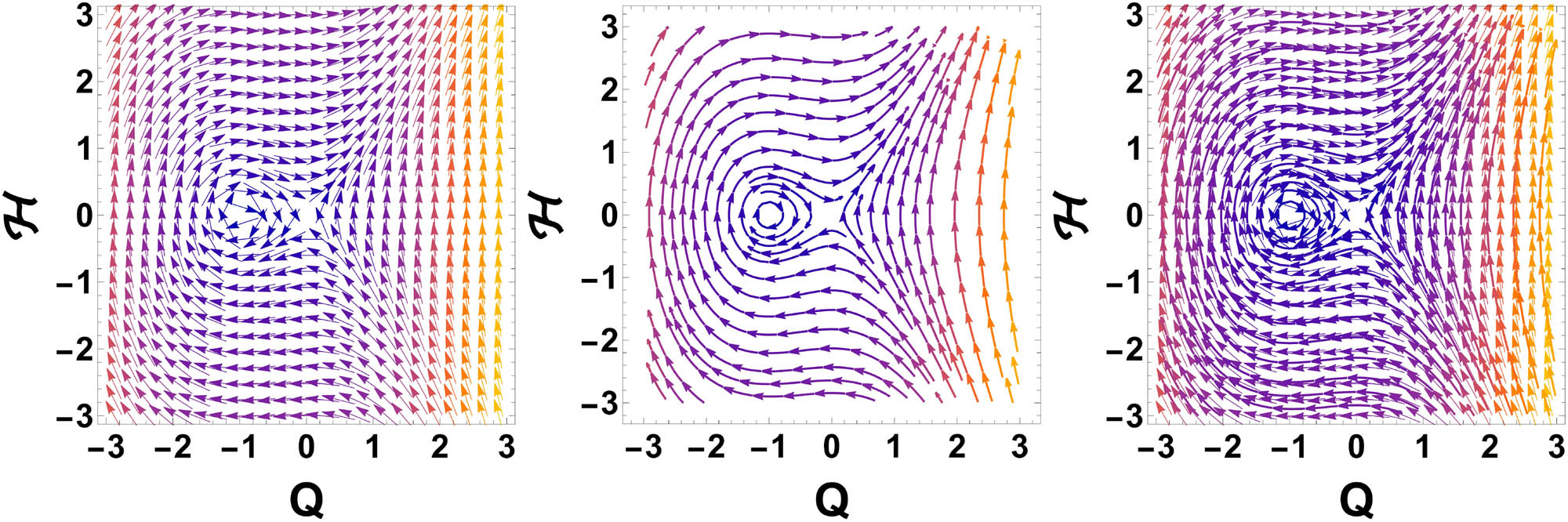
Case-3: When
By taking the parameters
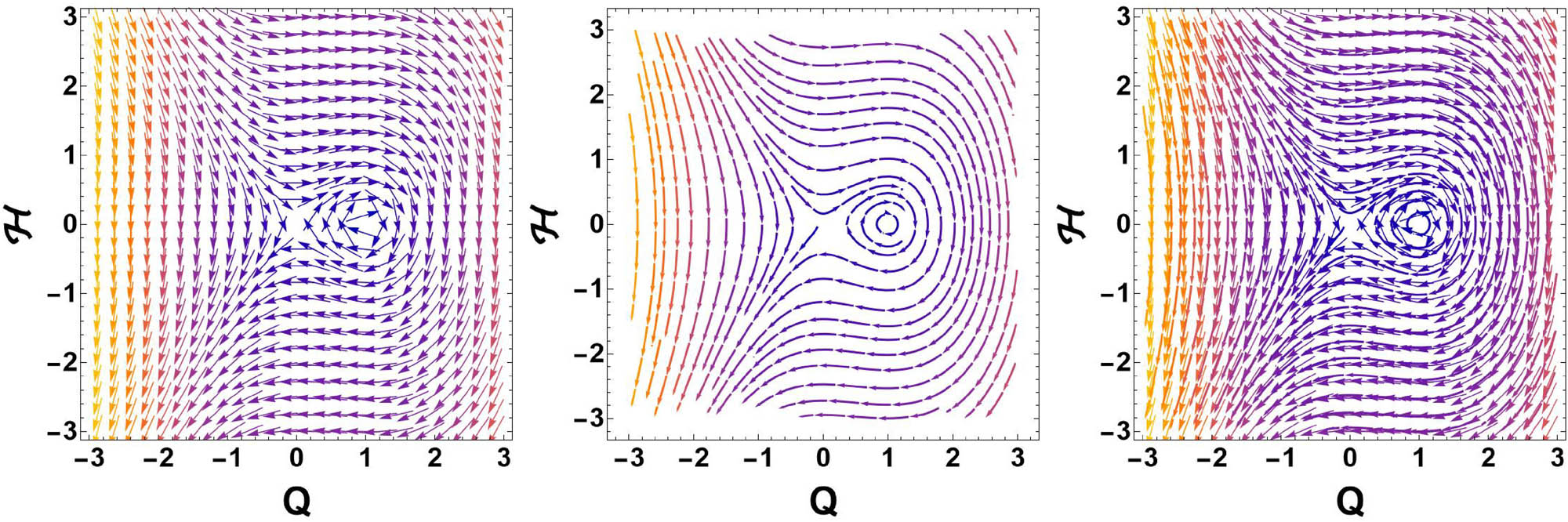
Case-4: When
By choosing the parameters
6 Stability analysis
For stability assessment, we utilize the concept of standard linear stability analysis [38] and here assume
where
On linearizing Eq. (56) in terms of
For further proceeding, we take the solutions of Eq. (57) as
where the normalized wave number and frequency of perturbation are denoted by
By inserting Eq. (58) into Eq. (57), we have
The dispersion relation, in terms of
The dispersion relation obtained in Eq. (60) is illustrated in Figure 9. If the wave number
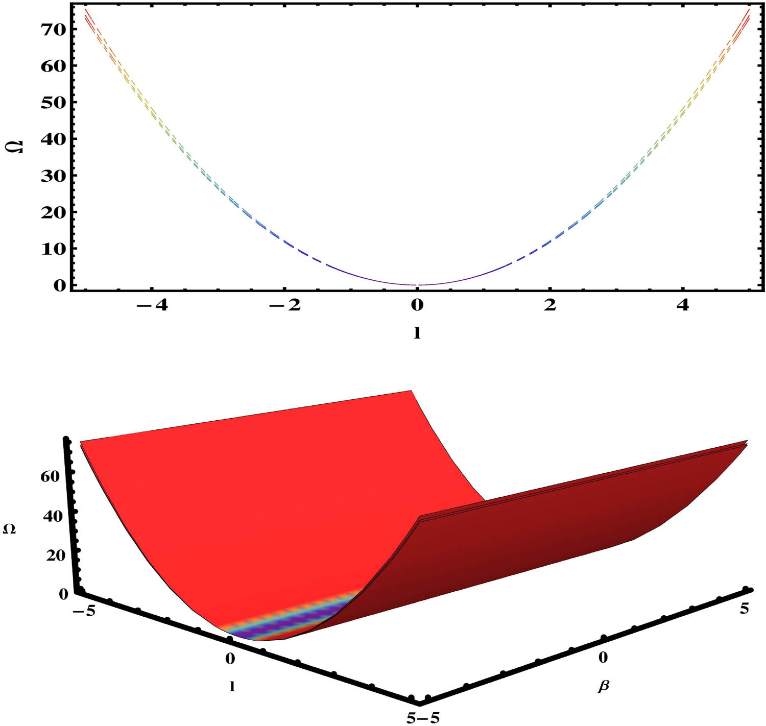
The dispersion relation between frequency
7 Results and discussion
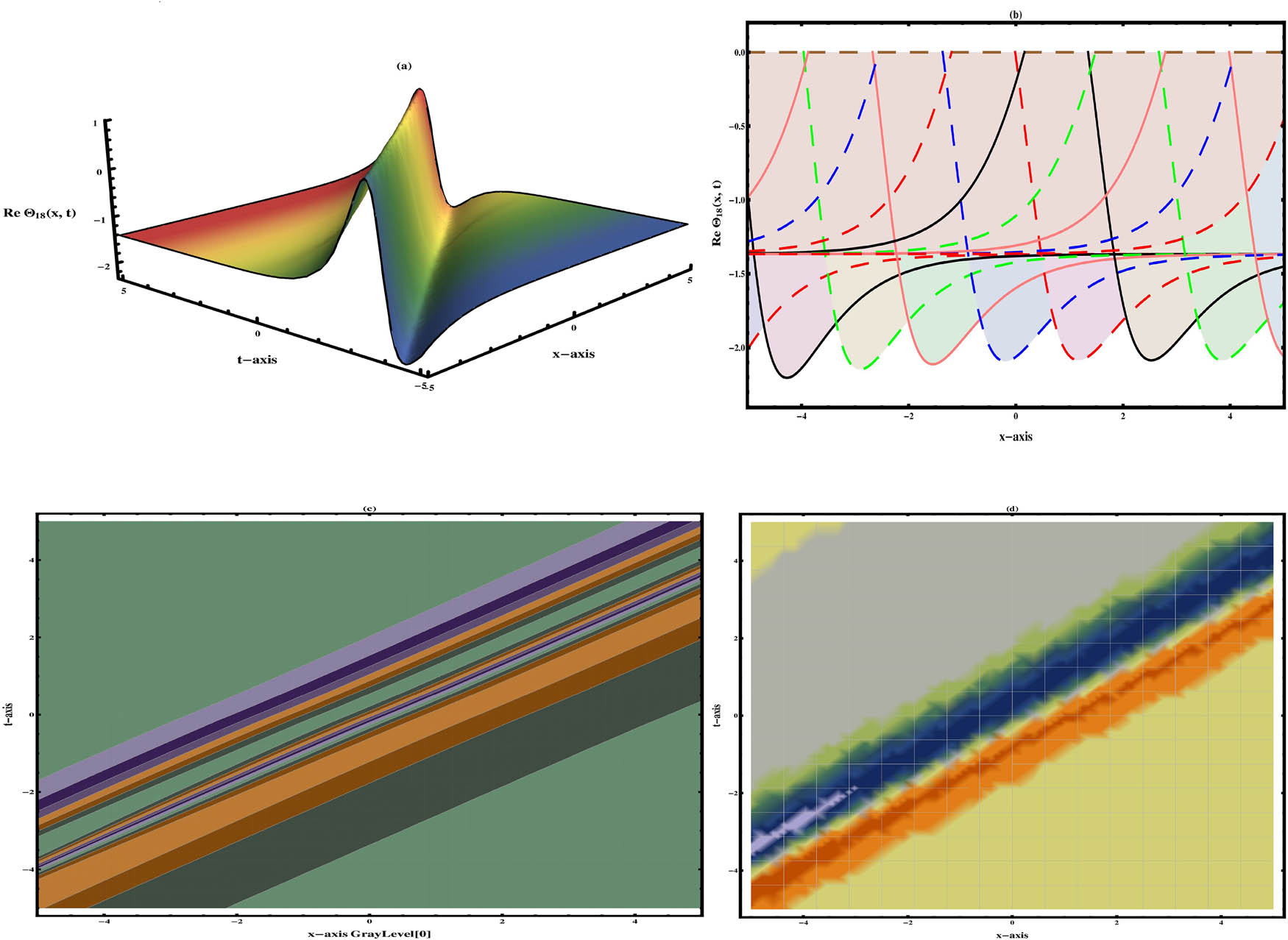
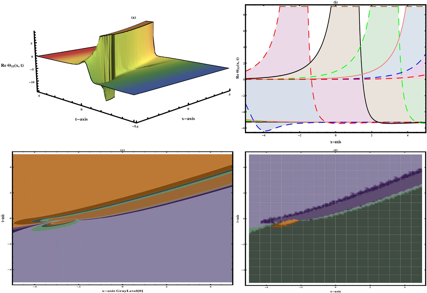
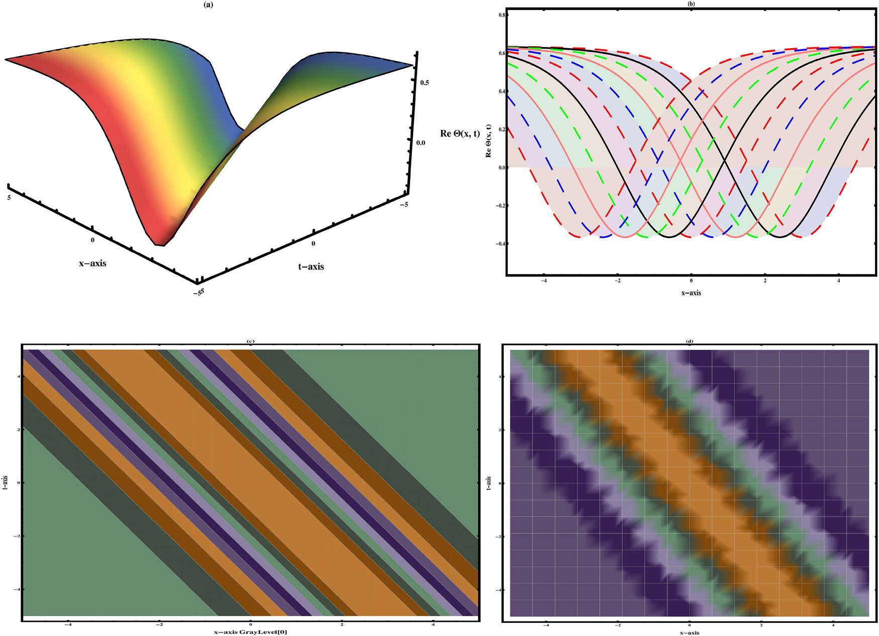
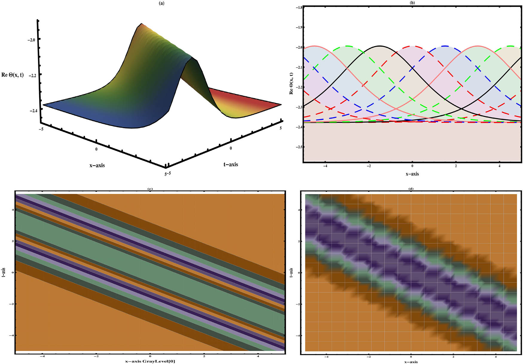
In this section, we discuss the outcomes of our proposed model and provide physical interpretations. It focuses on finding interesting, more generalized, and novel exact wave structures, including hyperbolic, trigonometric, complex hyperbolic, rational, bright, dark, singular, and singular periodic wave behaviors. Dark solitons exhibit greater stability and resistance to signal degradation compared to conventional solitons, despite their higher complexity in control. Bright solitons, meanwhile, are exemplified by their highest intensity, which surpasses the surrounding background levels. Another type, singular solitons, features abrupt discontinuities – often infinite – and may correspond to solitary waves with imaginary central positions. These singular shapes are particularly substantial in modeling rogue wave phenomena, where sudden, extreme amplitude spikes emerge. Moreover, periodic wave solutions characterize oscillatory forms that repeat at regular intervals, administrated by their wavelength and frequency. The period (time for one full cycle) and frequency (cycles per second) are defining parameters of such waveforms. These solutions have distinct physical interpretations, and we illustrate them graphically by choosing appropriate parameter values. These outcomes serve as inspiration for further research across different scientific fields, particularly in fluid dynamics. In the recent past, intensive work has been done on a given model. Li [23] retrieved solutions through the trial equation method. Taghizadeh et al [24] found exact traveling solutions with the aid of the homogeneous balance method. Kaplan et al. [25] discussed exact solutions and conservation laws via
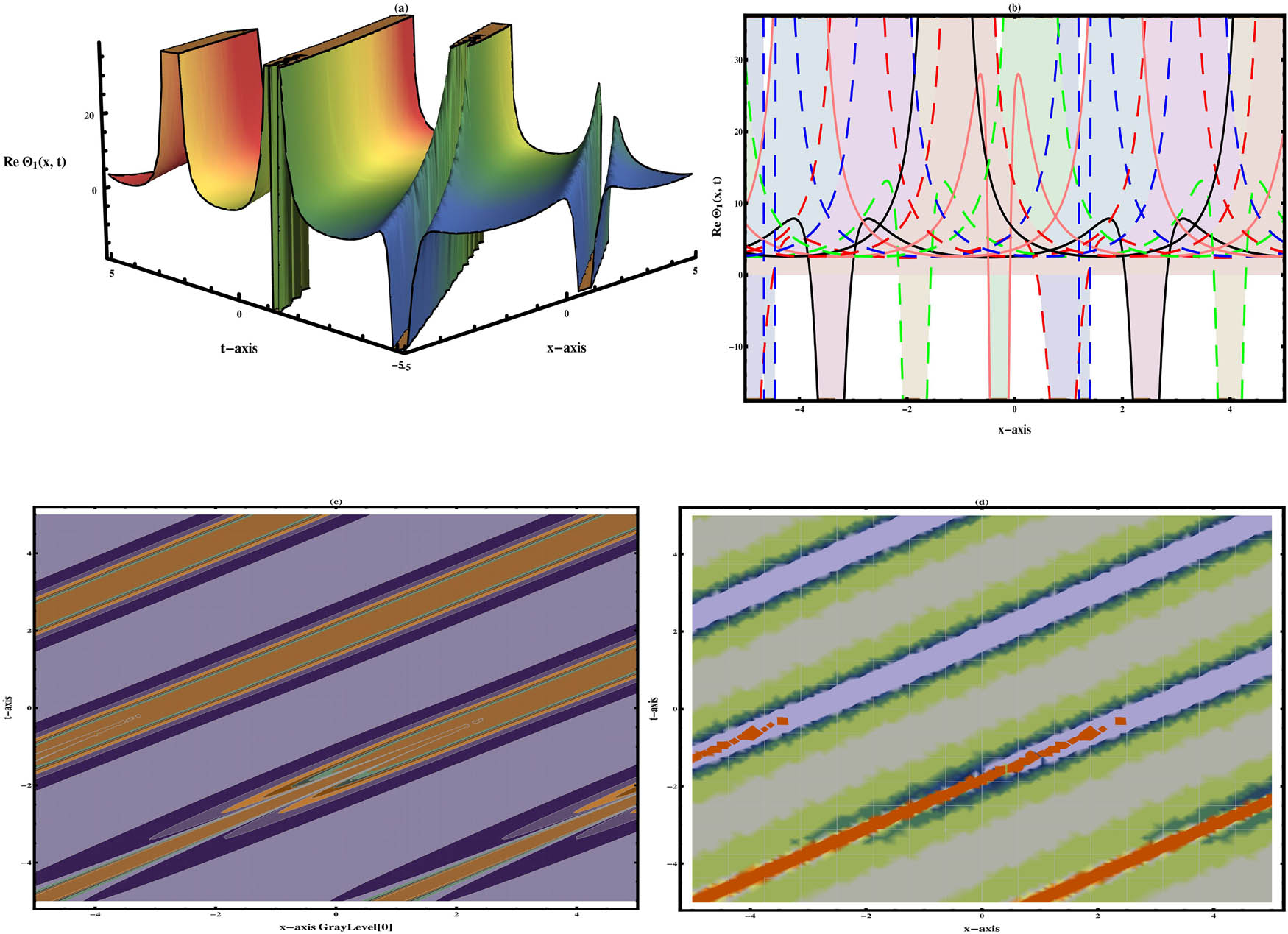
Visualization of Eq. (5) reveals the periodic wave structure under different arbitrary values

Visualization of Eq. (10) displays the dark wave structure under different arbitrary values

Visualization of Eq. (14) exhibits the dark-singular wave structure under different arbitrary values

Visualization of Eq. (20) exhibits the hyperbolic wave structure under different arbitrary values
Visualization of Eq. (22) shows the bright-dark wave structure under different arbitrary values
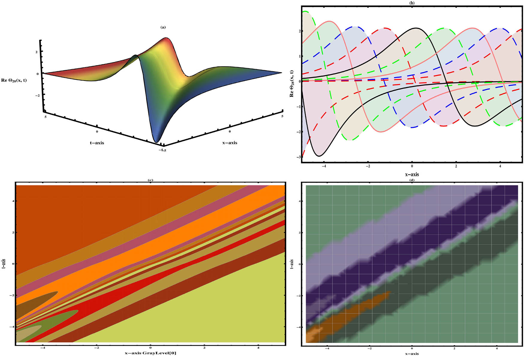
Visualization of Eq. (32) exhibits the bright-dark wave structure under different arbitrary values
Visualization of Eq. (37) shows the plane wave under different arbitrary values

Visualization of Eq. (44) shows the bright wave structure under different arbitrary values
Visualization of Eq. (47) shows the dark wave structure under different arbitrary values
Visualization of Eq. (50) shows the exponential wave structure under different arbitrary values
8 Concluding remarks
This study has investigated new exact traveling wave patterns for the time-FBO equation by using three efficient suggested computational techniques. These methods help us to uncover various exact solutions, including trigonometric, bright, dark singular, exponential, and their combined complex forms. We also observe singular periodic, plane-wave, and exponential solutions. Furthermore, we conduct stability analysis on the governed BO equations, confirming their high stability. Also, by amalgamating sensitivity, bifurcation, and stability analyses into our study, we can gain deeper insights into the behavior of the FBO equation and further authenticate the efficiency of the applied methodologies. The enduring stability of solitons, demonstrated as soliton pulses, travel through ideal lossless nonlinear fibers, mathematical physics, fluid dynamics, ocean engineering, and other deep-water nonlinear phenomena and highlight their potential integration into complex communication systems. We validate our results using Mathematica software, visually representing certain wave structures through 2D, 3D, contour, and density graphs with appropriate parameter values. Our findings illustrate the effectiveness of these aforementioned approaches in enhancing nonlinear dynamical behavior and suggest their potential application in uncovering diverse and novel soliton solutions for other NLPDEs encountered in mathematical physics and engineering. Through a comparative analysis of our newly developed solutions, it becomes evident that our proposed methods offer several advantages. They demonstrate strength, reliability, ease of implementation, and efficiency when applied to various NLPDEs. This makes it superior to previously utilized methods. The solutions obtained in this study will serve as a foundation for enhancing our understanding of water wave propagation in both shallow and deep water. This study displays a robust and methodical method for solving nonlinear fractional problems, leading to the discovery of novel exact solutions. Moving forward, we aim to expand the method’s versatility, with a concentration on tackling highly nonlinear systems, variable-coefficient models, and variable-order FPDEs. Furthermore, we will plan: (i) to extend these methodologies to other nonlinear fractional PDEs or consider higher-dimensional generalizations; (ii) to analyze the effects of noise term by adding the stochastic term in the governing equation; and (iii) to develop new numerical and analytical methods to solve FBO equations, enabling more accurate and efficient simulations.
Acknowledgments
The authors extend their appreciation to Taif University, Saudi Arabia, for supporting this work through project number (TU-DSPP-2024-70).
-
Funding information: This research was financially supported by Firat University.
-
Author contributions: Muhammad Bilal: methodology, software, and writing – original draft. Shafqat Ur Rehman: investigation, conceptualization, and writing – review and editing. Usman Younas: data curation, writing – review and editing, and visualization. Alsharef Mohammad: formal analysis, conceptualization, and funding acquisition. Shahram Rezapoure: formal analysis, data curation, and conceptualization. Mustafa Inc: resources, validation, and writing – review and editing. All authors have accepted responsibility for the entire content of this manuscript and approved its submission.
-
Conflict of interest: The authors state no conflict of interest.
-
Data availability statement: All data generated or analyzed during this study are included in this published article.
References
[1] Mandal UK, Malik S, Kumar S, Das A. A generalized (2+1)-dimensional Hirota bilinear equation: integrability, solitons and invariant solutions. Nonlinear Dyn. 2023;111(5):4593–611. 10.1007/s11071-022-08036-8Suche in Google Scholar
[2] Ying L, Li M, Shi Y. New exact solutions and related dynamic behaviors of a (3+1)-dimensional generalized Kadomtsev-Petviashvili equation. Nonlinear Dyn. 2024;112(13):11349–72. 10.1007/s11071-024-09539-2Suche in Google Scholar
[3] Rezazadeh H, Younis M, Eslami M, Bilal M, Younas U. New exact traveling wave solutions to the (2+1)-dimensional Chiral nonlinear Schrödinger equation. Math Model Nat Phenom. 2021;16:38. 10.1051/mmnp/2021001Suche in Google Scholar
[4] Eslami M, Rezazadeh H. The first integral method for Wu-Zhang system with conformable time-fractional derivative. Calcolo. 2016;53(3):475–85. 10.1007/s10092-015-0158-8Suche in Google Scholar
[5] Wang KJ, Shi F, Wang GD. Abundant soliton structures to the (2+1)-dimensional Heisenberg ferromagnetic spin chain dynamical model. Adv Math Phys. 2023;2023(1):4348758. 10.1155/2023/4348758Suche in Google Scholar
[6] Bilal M, Seadawy AR, Younis M, Rizvi STR, Zahed H. Dispersive of propagation wave solutions to unidirectional shallow water wave Dullin-Gottwald-Holm system and modulation instability analysis. Math Methods Appl Sci. 2021;44(5):4094–104. 10.1002/mma.7013Suche in Google Scholar
[7] Guan X, Liu W, Zhou Q, Biswas A. Darboux transformation and analytic solutions for a generalized super-NLS-mKdV equation. Nonlinear Dyn. 2019;98(2):1491–500. 10.1007/s11071-019-05275-0Suche in Google Scholar
[8] Alruwaili AD, Seadawy AR, Iqbal M, Beinane SAO. Dust-acoustic solitary wave solutions for mixed nonlinearity modified Korteweg-de Vries dynamical equation via analytical mathematical methods. J Geom Phys. 2022;176:104504. 10.1016/j.geomphys.2022.104504Suche in Google Scholar
[9] Bilal M, Ren J, Inc M, Alqahtani RT. Dynamics of solitons and weakly ion-acoustic wave structures to the nonlinear dynamical model via analytical techniques. Opt Quantum Electron. 2023;55(7):656. 10.1007/s11082-023-04880-zSuche in Google Scholar
[10] Wang XB, Han B. Application of the Riemann-Hilbert method to the vector modified Korteweg-de Vries equation. Nonlinear Dyn. 2020;99(2):1363–77. 10.1007/s11071-019-05359-xSuche in Google Scholar
[11] Hussain A, Ibrahim TF, Birkea FMO, Al-Sinan BR. Dynamical behavior of analytical soliton solutions to the Kuralay equations via symbolic computation. Nonlinear Dyn. 2024;112(22):20231–54. 10.1007/s11071-024-10101-3Suche in Google Scholar
[12] Usman M, Hussain A, Abd El-Rahman M, Herrera J. Group theoretic approach to (4+1)-dimensional Boiti-Leon-Manna-Pempinelli equation. Alex Eng J. 2025;118:449–65. 10.1016/j.aej.2025.01.071Suche in Google Scholar
[13] Hussain A, Zaman FD, Ali H. Dynamic nature of analytical soliton solutions of the nonlinear ZKBBM and GZKBBM equations. Partial Differ Equ Appl Math. 2024;10:100670. 10.1016/j.padiff.2024.100670Suche in Google Scholar
[14] Jumarie G. Laplace’s transform of fractional order via the Mittag-Leffler function and modified Riemann-Liouville derivative. Appl Math Lett. 2009;22(11):1659–64. 10.1016/j.aml.2009.05.011Suche in Google Scholar
[15] Mozaffari FS, Hassanabadi H, Sobhani H, Chung WS. On the conformable fractional quantum mechanics. J Korean Phys Soc. 2018;72(9):980–6. 10.3938/jkps.72.980Suche in Google Scholar
[16] Cevikel AC. Traveling wave solutions of conformable Duffing model in shallow water waves. Int J Mod Phys B. 2022;36(25):2250164. 10.1142/S0217979222501648Suche in Google Scholar
[17] Chen C, Jiang YL. Simplest equation method for some time-fractional partial differential equations with conformable derivative. Comput Math Appl. 2018;75(8):2978–88. 10.1016/j.camwa.2018.01.025Suche in Google Scholar
[18] Kumar D, Kaplan M. New analytical solutions of (2+1)-dimensional conformable time fractional Zoomeron equation via two distinct techniques. Chin J Phys. 2018;56(5):2173–85. 10.1016/j.cjph.2018.09.013Suche in Google Scholar
[19] Benjamin TB. Internal waves of permanent form in fluids of great depth. J Fluid Mech. 1967;29(3):559–92. 10.1017/S002211206700103XSuche in Google Scholar
[20] Ono H. Algebraic solitary waves in stratified fluids. J Phys Soc Jpn. 1975;39(4):1082–91. 10.1143/JPSJ.39.1082Suche in Google Scholar
[21] Ewen JF, Gunshor RL, Weston VH. Surface acoustic solitons. Jpn J Appl Phys. 1980;19(S1):683. 10.7567/JJAPS.19S1.683Suche in Google Scholar
[22] Sagar B, Ray SS. A localized meshfree technique for solving fractional Benjamin-Ono equation describing long internal waves in deep stratified fluids. Commun Nonlinear Sci Numer Simul. 2023;123:107287. 10.1016/j.cnsns.2023.107287Suche in Google Scholar
[23] Li Y. Application of Trial Equation Method for Solving the Benjamin Ono Equation. J Appl Math Phys. 2014;2(3):45–9. 10.4236/jamp.2014.23005Suche in Google Scholar
[24] Taghizadeh N, Mirzazadeh M, Farahrooz F. Exact soliton solutions for second-order Benjamin-Ono equation. Appl Appl Math Int J. 2011;6(1):31. Suche in Google Scholar
[25] Kaplan M, San S, Bekir A. On the exact solutions and conservation laws to the Benjamin-Ono equation. J Appl Anal Comput. 2018;8(1):1–9. 10.11948/2018.1Suche in Google Scholar
[26] Zhen W, De-Sheng L, Hui-Fang L, Hong-Qing Z. A method for constructing exact solutions and application to Benjamin Ono equation. Chin Phys. 2005;14(11):2158. 10.1088/1009-1963/14/11/003Suche in Google Scholar
[27] Tasbozan O. New analytical solutions for time fractional Benjamin-Ono equation arising internal waves in deep water. China Ocean Eng. 2019;33(5):593–600. 10.1007/s13344-019-0057-xSuche in Google Scholar
[28] Mirhosseini-Alizamini SM, Rezazadeh H, Srinivasa K, Bekir A. New closed form solutions of the new coupled Konno-Oono equation using the new extended direct algebraic method. Pramana. 2020;94(1):52. 10.1007/s12043-020-1921-1Suche in Google Scholar
[29] Bhan C, Karwasra R, Malik S, Kumar S. Bifurcation, chaotic behavior, and soliton solutions to the KP-BBM equation through new Kudryashov and generalized Arnous methods. AIMS Math. 2024;9(4):8749–67. 10.3934/math.2024424Suche in Google Scholar
[30] Park C, Nuruddeen RI, Ali KK, Muhammad L, Osman MS, Baleanu D. Novel hyperbolic and exponential ansatz methods to the fractional fifth-order Korteweg-de Vries equations. Adv Differ Equ. 2020;2020(1):12. 10.1186/s13662-020-03087-wSuche in Google Scholar
[31] Bilal M, Ahmad J. New exact solitary wave solutions for the 3D-FWBBM model in arising shallow water waves by two analytical methods. Results Phys. 2021;25:104230. 10.1016/j.rinp.2021.104230Suche in Google Scholar
[32] Zulfiqar A, Ahmad J. Exact solitary wave solutions of fractional modified Camassa-Holm equation using an efficient method. Alex Eng J. 2020;59(5):3565–74. 10.1016/j.aej.2020.06.002Suche in Google Scholar
[33] Rehman SU, Bilal M, Ren J, Bayram M, Inc M. Sensitivity Analysis and Dynamics of Optical Dromions in Conformable Generalized Nonlinear Schrödinger Systems. Phys Lett A. 2024;531:130168. 10.1016/j.physleta.2024.130168Suche in Google Scholar
[34] Lu W, Ahmad J, Akram S, Aldwoah KA. Soliton solutions and sensitivity analysis to nonlinear wave model arising in optics. Phys Scr. 2024;99(8):085230. 10.1088/1402-4896/ad5fcdSuche in Google Scholar
[35] Islam SR, Khan K, Akbar MA. Optical soliton solutions, bifurcation, and stability analysis of the Chen-Lee-Liu model. Results Phys. 2023;51:106620. 10.1016/j.rinp.2023.106620Suche in Google Scholar
[36] ur Rahman M, Sun M, Boulaaras S, Baleanu D. Bifurcations, chaotic behavior, sensitivity analysis, and various soliton solutions for the extended nonlinear Schrödinger equation. Bound Value Probl. 2024;2024(1):15. 10.1186/s13661-024-01825-7Suche in Google Scholar
[37] Alazman I, Alkahtani BST, Mishra MN. Dynamic of bifurcation, chaotic structure and multi soliton of fractional nonlinear Schrödinger equation arise in plasma physics. Sci Rep. 2024;14(1):25781. 10.1038/s41598-024-72744-xSuche in Google Scholar PubMed PubMed Central
[38] Ali A, Ahmad J, Javed S. Stability analysis and novel complex solutions to the malaria model utilising conformable derivatives. Eur Phys J Plus. 2023;138(3):259. 10.1140/epjp/s13360-023-03851-3Suche in Google Scholar
© 2025 the author(s), published by De Gruyter
This work is licensed under the Creative Commons Attribution 4.0 International License.
Artikel in diesem Heft
- Research Articles
- Single-step fabrication of Ag2S/poly-2-mercaptoaniline nanoribbon photocathodes for green hydrogen generation from artificial and natural red-sea water
- Abundant new interaction solutions and nonlinear dynamics for the (3+1)-dimensional Hirota–Satsuma–Ito-like equation
- A novel gold and SiO2 material based planar 5-element high HPBW end-fire antenna array for 300 GHz applications
- Explicit exact solutions and bifurcation analysis for the mZK equation with truncated M-fractional derivatives utilizing two reliable methods
- Optical and laser damage resistance: Role of periodic cylindrical surfaces
- Numerical study of flow and heat transfer in the air-side metal foam partially filled channels of panel-type radiator under forced convection
- Water-based hybrid nanofluid flow containing CNT nanoparticles over an extending surface with velocity slips, thermal convective, and zero-mass flux conditions
- Dynamical wave structures for some diffusion--reaction equations with quadratic and quartic nonlinearities
- Solving an isotropic grey matter tumour model via a heat transfer equation
- Study on the penetration protection of a fiber-reinforced composite structure with CNTs/GFP clip STF/3DKevlar
- Influence of Hall current and acoustic pressure on nanostructured DPL thermoelastic plates under ramp heating in a double-temperature model
- Applications of the Belousov–Zhabotinsky reaction–diffusion system: Analytical and numerical approaches
- AC electroosmotic flow of Maxwell fluid in a pH-regulated parallel-plate silica nanochannel
- Interpreting optical effects with relativistic transformations adopting one-way synchronization to conserve simultaneity and space–time continuity
- Modeling and analysis of quantum communication channel in airborne platforms with boundary layer effects
- Theoretical and numerical investigation of a memristor system with a piecewise memductance under fractal–fractional derivatives
- Tuning the structure and electro-optical properties of α-Cr2O3 films by heat treatment/La doping for optoelectronic applications
- High-speed multi-spectral explosion temperature measurement using golden-section accelerated Pearson correlation algorithm
- Dynamic behavior and modulation instability of the generalized coupled fractional nonlinear Helmholtz equation with cubic–quintic term
- Study on the duration of laser-induced air plasma flash near thin film surface
- Exploring the dynamics of fractional-order nonlinear dispersive wave system through homotopy technique
- The mechanism of carbon monoxide fluorescence inside a femtosecond laser-induced plasma
- Numerical solution of a nonconstant coefficient advection diffusion equation in an irregular domain and analyses of numerical dispersion and dissipation
- Numerical examination of the chemically reactive MHD flow of hybrid nanofluids over a two-dimensional stretching surface with the Cattaneo–Christov model and slip conditions
- Impacts of sinusoidal heat flux and embraced heated rectangular cavity on natural convection within a square enclosure partially filled with porous medium and Casson-hybrid nanofluid
- Stability analysis of unsteady ternary nanofluid flow past a stretching/shrinking wedge
- Solitonic wave solutions of a Hamiltonian nonlinear atom chain model through the Hirota bilinear transformation method
- Bilinear form and soltion solutions for (3+1)-dimensional negative-order KdV-CBS equation
- Solitary chirp pulses and soliton control for variable coefficients cubic–quintic nonlinear Schrödinger equation in nonuniform management system
- Influence of decaying heat source and temperature-dependent thermal conductivity on photo-hydro-elasto semiconductor media
- Dissipative disorder optimization in the radiative thin film flow of partially ionized non-Newtonian hybrid nanofluid with second-order slip condition
- Bifurcation, chaotic behavior, and traveling wave solutions for the fractional (4+1)-dimensional Davey–Stewartson–Kadomtsev–Petviashvili model
- New investigation on soliton solutions of two nonlinear PDEs in mathematical physics with a dynamical property: Bifurcation analysis
- Mathematical analysis of nanoparticle type and volume fraction on heat transfer efficiency of nanofluids
- Creation of single-wing Lorenz-like attractors via a ten-ninths-degree term
- Optical soliton solutions, bifurcation analysis, chaotic behaviors of nonlinear Schrödinger equation and modulation instability in optical fiber
- Chaotic dynamics and some solutions for the (n + 1)-dimensional modified Zakharov–Kuznetsov equation in plasma physics
- Fractal formation and chaotic soliton phenomena in nonlinear conformable Heisenberg ferromagnetic spin chain equation
- Single-step fabrication of Mn(iv) oxide-Mn(ii) sulfide/poly-2-mercaptoaniline porous network nanocomposite for pseudo-supercapacitors and charge storage
- Novel constructed dynamical analytical solutions and conserved quantities of the new (2+1)-dimensional KdV model describing acoustic wave propagation
- Tavis–Cummings model in the presence of a deformed field and time-dependent coupling
- Spinning dynamics of stress-dependent viscosity of generalized Cross-nonlinear materials affected by gravitationally swirling disk
- Design and prediction of high optical density photovoltaic polymers using machine learning-DFT studies
- Robust control and preservation of quantum steering, nonlocality, and coherence in open atomic systems
- Coating thickness and process efficiency of reverse roll coating using a magnetized hybrid nanomaterial flow
- Dynamic analysis, circuit realization, and its synchronization of a new chaotic hyperjerk system
- Decoherence of steerability and coherence dynamics induced by nonlinear qubit–cavity interactions
- Finite element analysis of turbulent thermal enhancement in grooved channels with flat- and plus-shaped fins
- Modulational instability and associated ion-acoustic modulated envelope solitons in a quantum plasma having ion beams
- Statistical inference of constant-stress partially accelerated life tests under type II generalized hybrid censored data from Burr III distribution
- On solutions of the Dirac equation for 1D hydrogenic atoms or ions
- Entropy optimization for chemically reactive magnetized unsteady thin film hybrid nanofluid flow on inclined surface subject to nonlinear mixed convection and variable temperature
- Stability analysis, circuit simulation, and color image encryption of a novel four-dimensional hyperchaotic model with hidden and self-excited attractors
- A high-accuracy exponential time integration scheme for the Darcy–Forchheimer Williamson fluid flow with temperature-dependent conductivity
- Novel analysis of fractional regularized long-wave equation in plasma dynamics
- Development of a photoelectrode based on a bismuth(iii) oxyiodide/intercalated iodide-poly(1H-pyrrole) rough spherical nanocomposite for green hydrogen generation
- Investigation of solar radiation effects on the energy performance of the (Al2O3–CuO–Cu)/H2O ternary nanofluidic system through a convectively heated cylinder
- Quantum resources for a system of two atoms interacting with a deformed field in the presence of intensity-dependent coupling
- Studying bifurcations and chaotic dynamics in the generalized hyperelastic-rod wave equation through Hamiltonian mechanics
- A new numerical technique for the solution of time-fractional nonlinear Klein–Gordon equation involving Atangana–Baleanu derivative using cubic B-spline functions
- Interaction solutions of high-order breathers and lumps for a (3+1)-dimensional conformable fractional potential-YTSF-like model
- Hydraulic fracturing radioactive source tracing technology based on hydraulic fracturing tracing mechanics model
- Numerical solution and stability analysis of non-Newtonian hybrid nanofluid flow subject to exponential heat source/sink over a Riga sheet
- Numerical investigation of mixed convection and viscous dissipation in couple stress nanofluid flow: A merged Adomian decomposition method and Mohand transform
- Effectual quintic B-spline functions for solving the time fractional coupled Boussinesq–Burgers equation arising in shallow water waves
- Analysis of MHD hybrid nanofluid flow over cone and wedge with exponential and thermal heat source and activation energy
- Solitons and travelling waves structure for M-fractional Kairat-II equation using three explicit methods
- Impact of nanoparticle shapes on the heat transfer properties of Cu and CuO nanofluids flowing over a stretching surface with slip effects: A computational study
- Computational simulation of heat transfer and nanofluid flow for two-sided lid-driven square cavity under the influence of magnetic field
- Irreversibility analysis of a bioconvective two-phase nanofluid in a Maxwell (non-Newtonian) flow induced by a rotating disk with thermal radiation
- Hydrodynamic and sensitivity analysis of a polymeric calendering process for non-Newtonian fluids with temperature-dependent viscosity
- Exploring the peakon solitons molecules and solitary wave structure to the nonlinear damped Kortewege–de Vries equation through efficient technique
- Modeling and heat transfer analysis of magnetized hybrid micropolar blood-based nanofluid flow in Darcy–Forchheimer porous stenosis narrow arteries
- Activation energy and cross-diffusion effects on 3D rotating nanofluid flow in a Darcy–Forchheimer porous medium with radiation and convective heating
- Insights into chemical reactions occurring in generalized nanomaterials due to spinning surface with melting constraints
- Influence of a magnetic field on double-porosity photo-thermoelastic materials under Lord–Shulman theory
- Soliton-like solutions for a nonlinear doubly dispersive equation in an elastic Murnaghan's rod via Hirota's bilinear method
- Analytical and numerical investigation of exact wave patterns and chaotic dynamics in the extended improved Boussinesq equation
- Nonclassical correlation dynamics of Heisenberg XYZ states with (x, y)-spin--orbit interaction, x-magnetic field, and intrinsic decoherence effects
- Exact traveling wave and soliton solutions for chemotaxis model and (3+1)-dimensional Boiti–Leon–Manna–Pempinelli equation
- Unveiling the transformative role of samarium in ZnO: Exploring structural and optical modifications for advanced functional applications
- On the derivation of solitary wave solutions for the time-fractional Rosenau equation through two analytical techniques
- Analyzing the role of length and radius of MWCNTs in a nanofluid flow influenced by variable thermal conductivity and viscosity considering Marangoni convection
- Advanced mathematical analysis of heat and mass transfer in oscillatory micropolar bio-nanofluid flows via peristaltic waves and electroosmotic effects
- Exact bound state solutions of the radial Schrödinger equation for the Coulomb potential by conformable Nikiforov–Uvarov approach
- Some anisotropic and perfect fluid plane symmetric solutions of Einstein's field equations using killing symmetries
- Nonlinear dynamics of the dissipative ion-acoustic solitary waves in anisotropic rotating magnetoplasmas
- Curves in multiplicative equiaffine plane
- Exact solution of the three-dimensional (3D) Z2 lattice gauge theory
- Propagation properties of Airyprime pulses in relaxing nonlinear media
- Symbolic computation: Analytical solutions and dynamics of a shallow water wave equation in coastal engineering
- Wave propagation in nonlocal piezo-photo-hygrothermoelastic semiconductors subjected to heat and moisture flux
- Comparative reaction dynamics in rotating nanofluid systems: Quartic and cubic kinetics under MHD influence
- Laplace transform technique and probabilistic analysis-based hypothesis testing in medical and engineering applications
- Physical properties of ternary chloro-perovskites KTCl3 (T = Ge, Al) for optoelectronic applications
- Gravitational length stretching: Curvature-induced modulation of quantum probability densities
- The search for the cosmological cold dark matter axion – A new refined narrow mass window and detection scheme
- A comparative study of quantum resources in bipartite Lipkin–Meshkov–Glick model under DM interaction and Zeeman splitting
- PbO-doped K2O–BaO–Al2O3–B2O3–TeO2-glasses: Mechanical and shielding efficacy
- Nanospherical arsenic(iii) oxoiodide/iodide-intercalated poly(N-methylpyrrole) composite synthesis for broad-spectrum optical detection
- Sine power Burr X distribution with estimation and applications in physics and other fields
- Numerical modeling of enhanced reactive oxygen plasma in pulsed laser deposition of metal oxide thin films
- Dynamical analyses and dispersive soliton solutions to the nonlinear fractional model in stratified fluids
- Computation of exact analytical soliton solutions and their dynamics in advanced optical system
- An innovative approximation concerning the diffusion and electrical conductivity tensor at critical altitudes within the F-region of ionospheric plasma at low latitudes
- An analytical investigation to the (3+1)-dimensional Yu–Toda–Sassa–Fukuyama equation with dynamical analysis: Bifurcation
- Swirling-annular-flow-induced instability of a micro shell considering Knudsen number and viscosity effects
- Review Article
- Examination of the gamma radiation shielding properties of different clay and sand materials in the Adrar region
- Erratum
- Erratum to “On Soliton structures in optical fiber communications with Kundu–Mukherjee–Naskar model (Open Physics 2021;19:679–682)”
- Special Issue on Fundamental Physics from Atoms to Cosmos - Part II
- Possible explanation for the neutron lifetime puzzle
- Special Issue on Nanomaterial utilization and structural optimization - Part III
- Numerical investigation on fluid-thermal-electric performance of a thermoelectric-integrated helically coiled tube heat exchanger for coal mine air cooling
- Special Issue on Nonlinear Dynamics and Chaos in Physical Systems
- Analysis of the fractional relativistic isothermal gas sphere with application to neutron stars
- Abundant wave symmetries in the (3+1)-dimensional Chafee–Infante equation through the Hirota bilinear transformation technique
- Successive midpoint method for fractional differential equations with nonlocal kernels: Error analysis, stability, and applications
- Novel exact solitons to the fractional modified mixed-Korteweg--de Vries model with a stability analysis