
Curves in multiplicative equiaffine plane
-
Meltem Ogrenmis
 und
Emad E. Mahmoud
und
Emad E. Mahmoud

Abstract
In this study, we deal with multiplicative equiaffine plane curves. First, the concepts of multiplicative equiaffine arc length and multiplicative curvature are introduced. Multiplicative equiaffine Frenet formulas and an analog of the fundamental theorem are established. Finally, multiplicative equiaffine plane curves with constant multiplicative equiaffine curvature are classified.
1 Introduction
The foundational framework of classical analysis, which is extensively used in modern mathematical theory, was first developed by Leibniz and Newton toward the end of the seventeenth century, focusing on differential and integral calculus notations. Classical analysis builds upon core topics in trigonometry, algebra, and analytic geometry, encompassing key ideas such as limits, differentiation, integration, and series expansions. These operations are often viewed as basic and fundamental, akin to addition and subtraction, which is why classical analysis is sometimes referred to as summational analysis. Its applications are extensive, spanning a wide range of disciplines where precise mathematical modeling and the pursuit of optimal solutions are of great importance.
However, when dealing with phenomena governed by proportional change, scale invariance, or multiplicative growth and decay, the additive framework of classical analysis may not be the most natural or effective choice. This creates a gap in geometric modeling where multiplicative structures could provide a more accurate representation.
Despite its broad utility, classical analysis has limitations in certain mathematical contexts. Consequently, alternative frameworks have been developed that are founded on various arithmetic operations while maintaining classical analysis as a foundation. For example, during 1887, Volterra and Hostinsky introduced a novel analytical approach termed Volterra-type or multiplicative analysis, which is grounded in multiplication rather than addition as the primary operation [1]. In this framework, the operations of multiplication and division replace the roles traditionally assigned to addition and subtraction in classical analysis, offering a novel approach to mathematical modeling. This shift represents a fundamental rethinking of conventional analysis, where the relationships between variables are governed by multiplicative rather than additive structures. Between 1972 and 1983, Grossman and Katz expanded upon Volterra’s earlier contributions by formulating what became known as non-Newtonian analysis. This new analytical framework introduced innovative definitions and concepts, redefining how mathematical operations could be applied across various domains [2,3]. Collectively, these methodologies are known as geometric, bigeometric, and anageometric analysis, each offering unique perspectives and tools for addressing problems where classical approaches prove inadequate.
Multiplicative analysis, presented as a counterpart to classical analysis, has garnered increasing interest in the mathematical community, spurring further research and development. These alternative methods have shown potential in addressing a range of mathematical problems by exploring new structural frameworks. Consequently, they have enriched the scope of mathematical analysis and found applications in various fields.
In particular, the need to extend classical geometric frameworks – such as equiaffine differential geometry – into the multiplicative setting is motivated by the lack of a comprehensive theory that unifies multiplicative operations with affine invariance. Existing studies address either multiplicative analysis in general or classical equiaffine curves separately, but there is no systematic development of multiplicative equiaffine Frenet formulas, arc length, and curvature theory.
The recent surge of interest in multiplicative analysis is reflected in numerous mathematical studies. While a comprehensive listing is beyond the scope of this discussion, previous studies [4–8] have provided substantial contributions to the field. More recently, differential geometry has also incorporated multiplicative analysis. Notably, Georgiev advanced the study of multiplicative analysis with the publication of three key works [9–11]. These publications, particularly [10], are regarded as foundational texts in multiplicative geometry. They provide novel definitions and theorems that connect fundamental geometric structures with the principles of multiplicative analysis. In addition, these works highlight the relationships between multiplicative geometry and other mathematical fields, thereby providing valuable insights for researchers working in various areas of mathematics.
Furthering the development of geometric analysis, Nurkan and collaborators made significant advancements by applying geometric calculus to the derivation of Gram-Schmidt vectors [12]. In a related study, [13], spherical indicatrices and helices in non-Newtonian (multiplicative) Euclidean spaces are analyzed, offering new characterizations and examples. On the other hand, Aydın et al. provided a classification and visualization of rectifying curves within multiplicative Euclidean space, employing multiplicative spherical curves to illustrate their findings [14]. The study by Ceyhan et al. [15] extends these ideas to investigate tube surfaces using the algebra of multiplicative quaternions.
Other recent studies continue to apply non-Newtonian analysis to various branches of geometry. For instance, Has et al.’s work explores geometric approaches in the Lorentz-Minkowski space
On the topic of affine geometry, extensive research has been conducted on affine spaces and their properties. For an in-depth exploration of both fundamental and advanced topics within this domain, readers may refer to works such as [25–28], which offer detailed discussions of classical and modern perspectives on affine geometry.
Besides differential geometry, there are applications of multiplicative calculus in dynamical systems [29,30], in eco-nomics [31,32], and in image analysis [33,34].
In addition to its intrinsic mathematical elegance, equiaffine differential geometry holds significant relevance in various physical contexts. The equiaffine framework, which preserves volume under affine transformations, naturally aligns with the modeling of physical systems where volume preservation or density invariance is critical. For instance, in fluid mechanics, the behavior of incompressible flows can be more accurately described using equiaffine invariants. Similarly, in continuum mechanics, equiaffine structures provide a geometric interpretation of stress and strain in materials that undergo deformation without volume change. Moreover, affine-invariant quantities appear in general relativity and gauge theories, where they are associated with affine connections and energy-momentum distributions. These examples illustrate that equiaffine geometry is not merely an abstract mathematical construct but also a powerful analytical tool with substantial applicability in theoretical and applied physics.
The aim of this study is to bridge the gap between multiplicative analysis and equiaffine geometry by developing a complete multiplicative equiaffine framework for plane curves. The main contributions can be summarized as follows: (1) defining multiplicative equiaffine arc length and curvature, (2) deriving multiplicative equiaffine Frenet formulas and an analogue of the fundamental theorem, and (3) classifying plane curves with constant multiplicative equiaffine curvature. Such a framework is expected to have applications in modeling scale-invariant geometric phenomena in physics, continuum mechanics, and data science.
This study is organized as follows: first, the foundational concepts of multiplicative calculus are introduced. Next, essential aspects of equiaffine geometry relevant to the analysis are presented. Finally, the curvature of a multiplicative plane curve is computed, and curves with constant curvature are characterized.
The novelty of this study lies in the systematic development of a full-fledged differential geometry framework within a multiplicative equiaffine setting. Unlike prior studies, we provide explicit Frenet equations, arc-length formulations, and curvature characterizations based on multiplicative operations. This presents a foundational shift that invites new geometric intuition and theoretical development.
2 Preliminaries
In this section, we introduce two essential topics. The first subsection presents the basics of equiaffine plane curves, focusing on the determinant in the affine plane and the equi-affine arc-length. The second subsection introduces the concept of multiplicative analysis. We explore multiplicative operations and structures, including multiplicative addition, multiplication, and derivatives. Additionally, we define the multiplicative determinant as a logarithmic analogue of the classical determinant.
2.1 Basics of equiaffine plane curves
In this section, we will briefly discuss the fundamental concepts of equiaffine plane curves without going into detailed explanations.
Let
where
Let
The arc-length parameter
where
According to the fundamental theorem of equiaffine plane curves, a smooth function
2.2 Multiplicative analysis
In this section, we outline fundamental definitions and principles concerning multiplicative analysis, drawing insights from Georgiev’s works [9–11]. Following this, we will discuss multiplicative equiaffine plane curves.
Let
These operations form a multiplicative structure denoted by
The multiplicative zero and unit in
For
The multiplicative sine (
Similarly, multiplicative hyperbolic functions are given by
Let
where
For
Moreover, for two vectors
This represents a multiplicative analogue of the classical determinant and is defined in the space
3 Multiplicative equiaffine plane curves
In this section, we develop the theory of multiplicative equiaffine plane curves by defining the multiplicative affine plane and the multiplicative determinant, which generalizes area calculations. We also introduce key concepts like multiplicative linear independence, the multiplicative equiaffine group, and the multiplicative arc length. Furthermore, we present the multiplicative Frenet apparatus and the corresponding Frenet equations, which describe the curvature and frame transformations of these curves.
Definition 3.1
The multiplicative affine plane
where
Proposition 3.2
For vector fields
is satisfied.
Proof
Let’s assume
Then, the determinant of the matrix formed by
Now, let’s multiplicative differentiate this expression, then
is obtained. By using multiplicative derivative rule, we have
The right side of this expression is written as follows:
or
Therefore, we have proved the result.□
Definition 3.3
A pair
holds only when
Definition 3.4
A multiplicative nondegenerate smooth parametric curve in
for any
Definition 3.5
The multiplicative equiaffine arc length function
where
Proposition 3.6
The multiplicative equiaffine curvature
Proof
Consider
for all
If we differentiate Eq. (3.13) with respect to
which implies that
Therefore, we conclude the proof.□
Definition 3.7
Let
The multiplicative Frenet equations in the equiaffine sense are as follows:
It is obvious that the following occurs
The relations between the multiplicative equiaffine frames of
4 Plane curves of constant multiplicative equiaffine curvature
In this section, we classify the plane curves with constant multiplicative equiaffine curvature. Let
We seek to construct a curve
Substituting
To solve Eq. (4.2), we examine different cases:
(i)
The relation Eq. (4.2) give
for constant vectors
is obtained. The following relation is given by integrating Eq. (4.4)
for a constant vector
and hence, Eq. (4.5) is
(ii)
The relation Eq. (4.2) give
where
is obtained. Integrating Eq. (4.9), one obtains
for a constant vector
and Eq. (4.10) is
(iii)
By Eq. (4.2),
Analogously by similar approach with the previous case, we obtain
Thus, we have briefly proven following theorem.
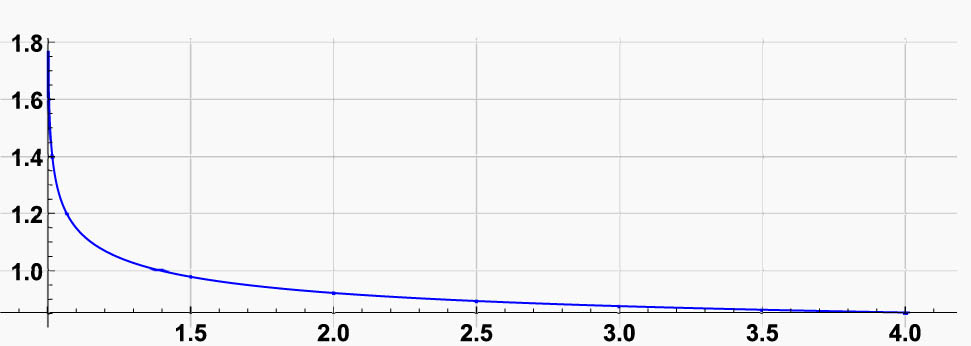
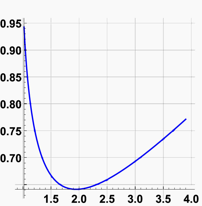
Theorem 4.1
Let
Then, the graphs of Eqs (4.7) and (4.12) are shown in Figures 1 and 2.
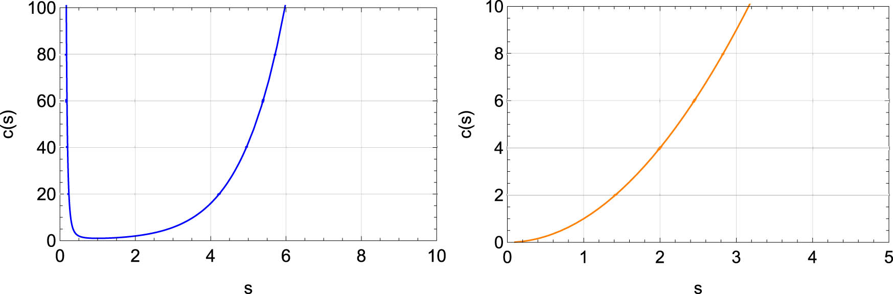
The curve describes a multiplicative parabola arising from the condition
A multiplicative ellipse corresponding to constant multiplicative equiaffine curvature
5 Multiplicative equiaffine curvature of plane curves with an arbitrary parameter
In the preceding section, plane curves parameterized by arc length were considered. Here, we generalize the setting and compute the multiplicative equiaffine curvature for plane curves equipped with an arbitrary parameter. A proposition is provided to facilitate the computation, and illustrative examples are given to clarify the method.
Proposition 5.1
Let
where
Proof
Let
is obtained. Here,
Thus,
is obtained. That is,
Now, let us compute the multiplicative curvature
From Eq. (5.4), that is, from
taking the multiplicative derivative once more yields
is obtained. Taking the multiplicative derivative once again gives
is obtained. Substituting Eqs (5.7) and (5.8) into Eq. (5.5) yields Eq. (5.1), and thus, the proposition is proved.□
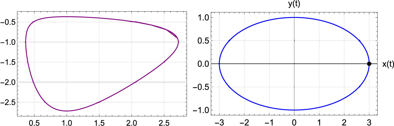
Example 1
Let
The graph of this curve is shown in Figure 3.
The curve
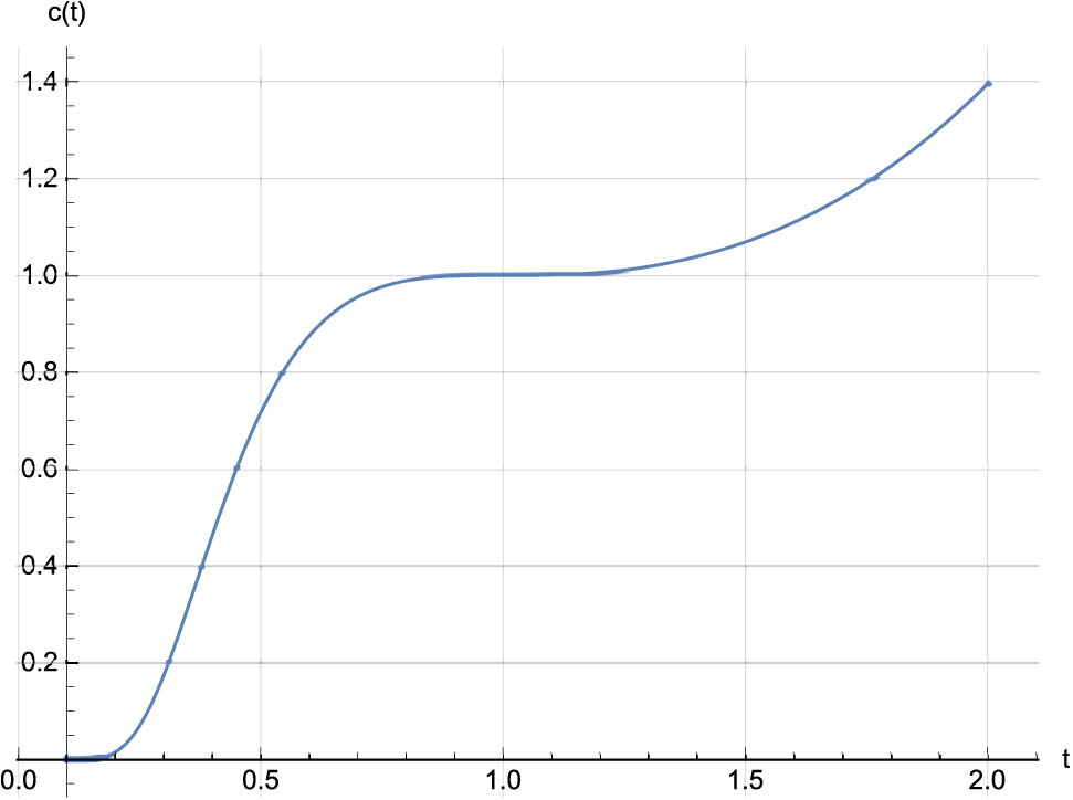
Example 2
Let
The graph of this curve is shown in Figure 4.
The curve
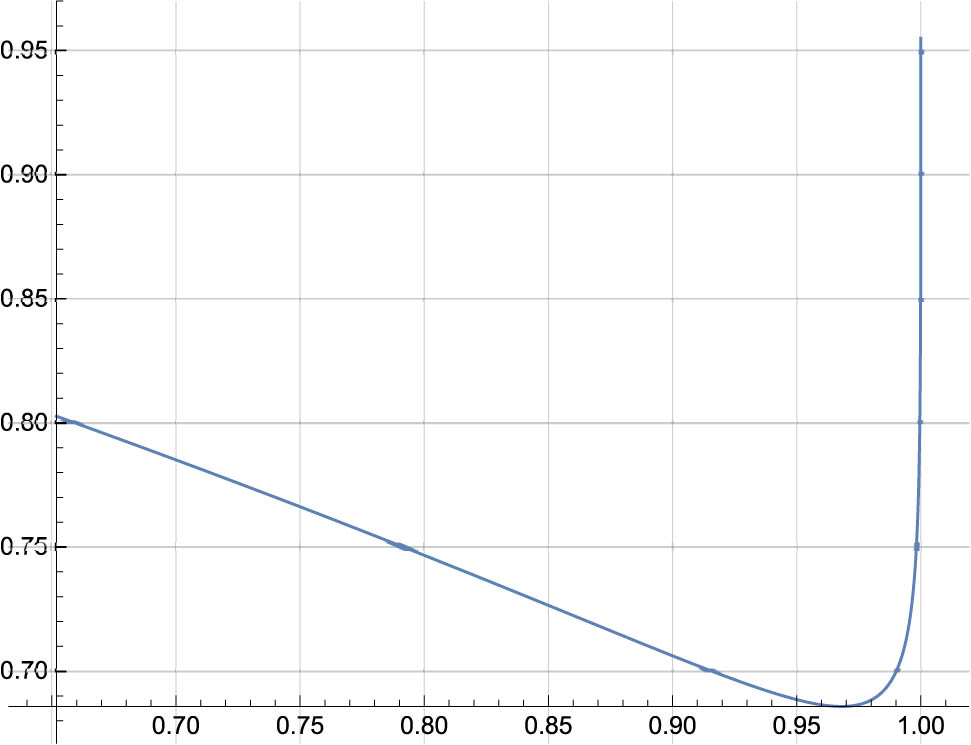
Example 3
Let
The graph of this curve is shown in Figure 5.
The curve
Example 4
Let
The graph of this curve is shown in Figure 6.
The curve
6 Discussion
Although this work is formulated in a purely mathematical framework, the use of multiplicative structures aligns with modeling approaches in physics, particularly in scale-invariant systems, exponential decay/growth models, and systems governed by proportional change. Such frameworks may appear in thermodynamics, population dynamics, or quantum models involving exponential operators. Potential applications of the proposed geometric model include areas where traditional additive calculus fails to provide natural descriptions – such as biological growth, economic systems under compounding interest, or dynamical systems characterized by proportional (rather than incremental) evolution. In addition, the structure can be useful in data science contexts involving multiplicative noise. Compared to classical equiaffine differential geometry, where additive operations govern the frame evolution, the proposed multiplicative approach replaces these operations with their exponential-logarithmic analogues. For instance, the multiplicative curvature is derived from logarithmic determinants, which offer a different perspective on area preservation and invariance under the multiplicative group
Acknowledgments
The authors extend their appreciation to Fırat University. This work was supported by Taif University, Saudi Arabia, through project number (TU-DSPP-2024-94).
-
Funding information: This research was funded by Fırat University and supported by Taif University, Saudi Arabia, Project No. (TU-DSPP-2024-94).
-
Author contributions: Meltem Ogrenmis: conceptualization; methodology; writing-original draft; visualization; investigation; Alper Osman Ogrenmis: formal analysis; literature review; writing-review and editing; manuscript revision; Emad E. Mahmoud: supervision; project administration; writing-review and editing. All authors have accepted responsibility for the entire content of this manuscript and approved its submission.
-
Conflict of interest: The authors state no conflict of interest.
-
Data availability statement: All data generated or analyzed during this study are included in this manuscript.
References
[1] Volterra V, Hostinsky B. Operations infinitesimales lineares. Paris: Herman; 1938. Suche in Google Scholar
[2] Grossman M, Katz R. Non-Newtonian calculus. 1st ed. Pigeon Cove, Massachusetts: Lee Press; 1972. Suche in Google Scholar
[3] Grossman M. Bigeometric calculus: A system with a scale-free derivative. Massachusetts: Archimedes Foundation; 1983. Suche in Google Scholar
[4] Stanley D. A multiplicative calculus. Primus. 1999;9(4):310–26. 10.1080/10511979908965937Suche in Google Scholar
[5] Bashirov A, Riza M. On complex multiplicative differentiation. TWMS J Appl Eng Math. 2011;1(1):75–85. Suche in Google Scholar
[6] Yazici M, Selvitopi H. Numerical methods for the multiplicative partial differential equations. Open Math. 2017;15:1344–50. 10.1515/math-2017-0113Suche in Google Scholar
[7] Yalçín N, Celik E. Solution of multiplicative homogeneous linear differential equations with constant exponentials. New Trends Math Sci. 2018;6(2):58–67. 10.20852/ntmsci.2018.270Suche in Google Scholar
[8] Goktas S, Kemaloglu H, Yilmaz E. Multiplicative conformable fractional Dirac system. Turkish J Math. 2022;46:973–90. 10.55730/1300-0098.3136Suche in Google Scholar
[9] Georgiev SG, Zennir K. Multiplicative differential calculus. 1st ed. New York: Chapman and Hall/CRC; 2022. 10.1201/9781003299080-1Suche in Google Scholar
[10] Georgiev SG. Multiplicative differential geometry. 1st ed. New York: Chapman and Hall/CRC; 2022. 10.1201/9781003299844-1Suche in Google Scholar
[11] Georgiev SG, Zennir K, Boukarou A. Multiplicative analytic geometry. 1st ed. New York: Chapman and Hall/CRC; 2022. 10.1201/9781003325284-1Suche in Google Scholar
[12] Nurkan SK, Gurgil I, Karacan MK. Vector properties of geometric calculus. Math Meth Appl Sci. 2023;46:17672–91. 10.1002/mma.9525Suche in Google Scholar
[13] Has A, Yílmaz B. On non-Newtonian helices in multiplicative Euclidean space. Fund Contemp Math Sci. 2025;6(2):196–217. 10.54974/fcmathsci.1644427Suche in Google Scholar
[14] Aydin ME, Has A, Yílmaz B. A non-Newtonian approach in differential geometry of curves: multiplicative rectifying curves, Bullet Korean Math Soc. 2024;61(3):849–66. Suche in Google Scholar
[15] Ceyhan H, Özdemir Z, Gök İ. Multiplicative generalized tube surfaces with multiplicative quaternions algebra. Math Meth Appl Sci. 2024;47:9157–68. 10.1002/mma.10065Suche in Google Scholar
[16] Has A, Yílmaz B, Yíldírím H. A non-Newtonian perspective on multiplicative Lorentz-Minkowski space L*3. Math Meth Appl Sci. 2024;47:13875–888. 10.1002/mma.10243Suche in Google Scholar
[17] Özdemir Z, Ceyhan H. Multiplicative hyperbolic split quaternions and generating geometric hyperbolical rotation matrices. Appl Math Comput. 2024;479:128862. 10.1016/j.amc.2024.128862Suche in Google Scholar
[18] Has A, Yílmaz B. A non-Newtonian conics in multiplicative analytic geometry. Turkish J Math. 2024;48(5):976–94. 10.55730/1300-0098.3554Suche in Google Scholar
[19] Es H. Plane kinematics in homothetic multiplicative calculus. J Univ Math. 2024;7(1):37–47. 10.33773/jum.1408506Suche in Google Scholar
[20] Has A, Yílmaz B. A non-Newtonian magnetic curves in multiplicative Riemann manifolds. Phys Scr. 2024;99(4):045238. 10.1088/1402-4896/ad32b7Suche in Google Scholar
[21] Aydin ME, Has A, Yílmaz B. Multiplicative rectifying submanifolds of multiplicative Euclidean space. Math Meth Appl Sci. 2025;48:329–39. 10.1002/mma.10329Suche in Google Scholar
[22] Broscateanu SC, Mihai A, Olteanu A. A note on the infinitesimal bending of a rectifying curve. Symmetry. 2024;16(10):1361. 10.3390/sym16101361. Suche in Google Scholar
[23] Burlacu A, Mihai A. Applications of differential geometry of curves in roads design. Rom J Trans Infrastruct. 2023;12(2):1–13, 10.2478/rjti-2023-0010. Suche in Google Scholar
[24] Jianu M, Achimescu S, Dăauş L, Mierluş-Mazilu I, Mihai A, Tudor D. On a surface associated to the catalan triangle. Axioms. 2022;11(12):685. 10.3390/axioms11120685Suche in Google Scholar
[25] Aydin ME, Mihai A, Yokus A. Applications of fractional calculus in equiaffine geometry: plane curves with fractional order. Math Meth Appl Sci. 2021;44:13659–69. 10.1002/mma.7649Suche in Google Scholar
[26] Davis D. Generic affine differential geometry of curves in Rn. Proc R Soc Edinburgh A. 2006;136:1195–205. 10.1017/S0308210500004947Suche in Google Scholar
[27] Guggenheimer HW. Differential geometry. New York: McGraw-Hill; 1963. Suche in Google Scholar
[28] Nomizu K, Sasaki T. Affine differential geometry: Geometry of affine immersions. Cambridge Tracts in Mathematics. Cambridge: Cambridge University Press; 1994. Suche in Google Scholar
[29] Aniszewska D, Rybaczuk M. Analysis of the multiplicative Lorenz system. Chaos Solitons Fract. 2005;25(1):79–90. 10.1016/j.chaos.2004.09.060Suche in Google Scholar
[30] Aniszewska D, Rybaczuk M. Lyapunov type stability and Lyapunov exponent for exemplary multiplicative dynamical systems. Nonlinear Dyn. 2008;54:345–54. 10.1007/s11071-008-9333-7Suche in Google Scholar
[31] Cordova-Lepe F. The multiplicative derivative as a measure of elasticity in economics. TEMAT-Theaeteto Atheniensi Math. 2006;2(3):7. Suche in Google Scholar
[32] Filip DA, Piatecki C. A non-newtonian examination of the theory of exogenous economic growth. Math. Aeterna. 2014;4:101–17. Suche in Google Scholar
[33] Florack L, Van Assen H. Multiplicative calculus in biomedical image analysis. J. Math. Imaging. Vis. 2012;42:64–75. 10.1007/s10851-011-0275-1Suche in Google Scholar
[34] Mora M, Cordova-Lepe F, Del-Valle R. A non-Newtonian gradient for contour detection in images with multiplicative noise. Pattern Recogn Lett. 2012;33(10):1245–56. 10.1016/j.patrec.2012.02.012Suche in Google Scholar
© 2025 the author(s), published by De Gruyter
This work is licensed under the Creative Commons Attribution 4.0 International License.
Artikel in diesem Heft
- Research Articles
- Single-step fabrication of Ag2S/poly-2-mercaptoaniline nanoribbon photocathodes for green hydrogen generation from artificial and natural red-sea water
- Abundant new interaction solutions and nonlinear dynamics for the (3+1)-dimensional Hirota–Satsuma–Ito-like equation
- A novel gold and SiO2 material based planar 5-element high HPBW end-fire antenna array for 300 GHz applications
- Explicit exact solutions and bifurcation analysis for the mZK equation with truncated M-fractional derivatives utilizing two reliable methods
- Optical and laser damage resistance: Role of periodic cylindrical surfaces
- Numerical study of flow and heat transfer in the air-side metal foam partially filled channels of panel-type radiator under forced convection
- Water-based hybrid nanofluid flow containing CNT nanoparticles over an extending surface with velocity slips, thermal convective, and zero-mass flux conditions
- Dynamical wave structures for some diffusion--reaction equations with quadratic and quartic nonlinearities
- Solving an isotropic grey matter tumour model via a heat transfer equation
- Study on the penetration protection of a fiber-reinforced composite structure with CNTs/GFP clip STF/3DKevlar
- Influence of Hall current and acoustic pressure on nanostructured DPL thermoelastic plates under ramp heating in a double-temperature model
- Applications of the Belousov–Zhabotinsky reaction–diffusion system: Analytical and numerical approaches
- AC electroosmotic flow of Maxwell fluid in a pH-regulated parallel-plate silica nanochannel
- Interpreting optical effects with relativistic transformations adopting one-way synchronization to conserve simultaneity and space–time continuity
- Modeling and analysis of quantum communication channel in airborne platforms with boundary layer effects
- Theoretical and numerical investigation of a memristor system with a piecewise memductance under fractal–fractional derivatives
- Tuning the structure and electro-optical properties of α-Cr2O3 films by heat treatment/La doping for optoelectronic applications
- High-speed multi-spectral explosion temperature measurement using golden-section accelerated Pearson correlation algorithm
- Dynamic behavior and modulation instability of the generalized coupled fractional nonlinear Helmholtz equation with cubic–quintic term
- Study on the duration of laser-induced air plasma flash near thin film surface
- Exploring the dynamics of fractional-order nonlinear dispersive wave system through homotopy technique
- The mechanism of carbon monoxide fluorescence inside a femtosecond laser-induced plasma
- Numerical solution of a nonconstant coefficient advection diffusion equation in an irregular domain and analyses of numerical dispersion and dissipation
- Numerical examination of the chemically reactive MHD flow of hybrid nanofluids over a two-dimensional stretching surface with the Cattaneo–Christov model and slip conditions
- Impacts of sinusoidal heat flux and embraced heated rectangular cavity on natural convection within a square enclosure partially filled with porous medium and Casson-hybrid nanofluid
- Stability analysis of unsteady ternary nanofluid flow past a stretching/shrinking wedge
- Solitonic wave solutions of a Hamiltonian nonlinear atom chain model through the Hirota bilinear transformation method
- Bilinear form and soltion solutions for (3+1)-dimensional negative-order KdV-CBS equation
- Solitary chirp pulses and soliton control for variable coefficients cubic–quintic nonlinear Schrödinger equation in nonuniform management system
- Influence of decaying heat source and temperature-dependent thermal conductivity on photo-hydro-elasto semiconductor media
- Dissipative disorder optimization in the radiative thin film flow of partially ionized non-Newtonian hybrid nanofluid with second-order slip condition
- Bifurcation, chaotic behavior, and traveling wave solutions for the fractional (4+1)-dimensional Davey–Stewartson–Kadomtsev–Petviashvili model
- New investigation on soliton solutions of two nonlinear PDEs in mathematical physics with a dynamical property: Bifurcation analysis
- Mathematical analysis of nanoparticle type and volume fraction on heat transfer efficiency of nanofluids
- Creation of single-wing Lorenz-like attractors via a ten-ninths-degree term
- Optical soliton solutions, bifurcation analysis, chaotic behaviors of nonlinear Schrödinger equation and modulation instability in optical fiber
- Chaotic dynamics and some solutions for the (n + 1)-dimensional modified Zakharov–Kuznetsov equation in plasma physics
- Fractal formation and chaotic soliton phenomena in nonlinear conformable Heisenberg ferromagnetic spin chain equation
- Single-step fabrication of Mn(iv) oxide-Mn(ii) sulfide/poly-2-mercaptoaniline porous network nanocomposite for pseudo-supercapacitors and charge storage
- Novel constructed dynamical analytical solutions and conserved quantities of the new (2+1)-dimensional KdV model describing acoustic wave propagation
- Tavis–Cummings model in the presence of a deformed field and time-dependent coupling
- Spinning dynamics of stress-dependent viscosity of generalized Cross-nonlinear materials affected by gravitationally swirling disk
- Design and prediction of high optical density photovoltaic polymers using machine learning-DFT studies
- Robust control and preservation of quantum steering, nonlocality, and coherence in open atomic systems
- Coating thickness and process efficiency of reverse roll coating using a magnetized hybrid nanomaterial flow
- Dynamic analysis, circuit realization, and its synchronization of a new chaotic hyperjerk system
- Decoherence of steerability and coherence dynamics induced by nonlinear qubit–cavity interactions
- Finite element analysis of turbulent thermal enhancement in grooved channels with flat- and plus-shaped fins
- Modulational instability and associated ion-acoustic modulated envelope solitons in a quantum plasma having ion beams
- Statistical inference of constant-stress partially accelerated life tests under type II generalized hybrid censored data from Burr III distribution
- On solutions of the Dirac equation for 1D hydrogenic atoms or ions
- Entropy optimization for chemically reactive magnetized unsteady thin film hybrid nanofluid flow on inclined surface subject to nonlinear mixed convection and variable temperature
- Stability analysis, circuit simulation, and color image encryption of a novel four-dimensional hyperchaotic model with hidden and self-excited attractors
- A high-accuracy exponential time integration scheme for the Darcy–Forchheimer Williamson fluid flow with temperature-dependent conductivity
- Novel analysis of fractional regularized long-wave equation in plasma dynamics
- Development of a photoelectrode based on a bismuth(iii) oxyiodide/intercalated iodide-poly(1H-pyrrole) rough spherical nanocomposite for green hydrogen generation
- Investigation of solar radiation effects on the energy performance of the (Al2O3–CuO–Cu)/H2O ternary nanofluidic system through a convectively heated cylinder
- Quantum resources for a system of two atoms interacting with a deformed field in the presence of intensity-dependent coupling
- Studying bifurcations and chaotic dynamics in the generalized hyperelastic-rod wave equation through Hamiltonian mechanics
- A new numerical technique for the solution of time-fractional nonlinear Klein–Gordon equation involving Atangana–Baleanu derivative using cubic B-spline functions
- Interaction solutions of high-order breathers and lumps for a (3+1)-dimensional conformable fractional potential-YTSF-like model
- Hydraulic fracturing radioactive source tracing technology based on hydraulic fracturing tracing mechanics model
- Numerical solution and stability analysis of non-Newtonian hybrid nanofluid flow subject to exponential heat source/sink over a Riga sheet
- Numerical investigation of mixed convection and viscous dissipation in couple stress nanofluid flow: A merged Adomian decomposition method and Mohand transform
- Effectual quintic B-spline functions for solving the time fractional coupled Boussinesq–Burgers equation arising in shallow water waves
- Analysis of MHD hybrid nanofluid flow over cone and wedge with exponential and thermal heat source and activation energy
- Solitons and travelling waves structure for M-fractional Kairat-II equation using three explicit methods
- Impact of nanoparticle shapes on the heat transfer properties of Cu and CuO nanofluids flowing over a stretching surface with slip effects: A computational study
- Computational simulation of heat transfer and nanofluid flow for two-sided lid-driven square cavity under the influence of magnetic field
- Irreversibility analysis of a bioconvective two-phase nanofluid in a Maxwell (non-Newtonian) flow induced by a rotating disk with thermal radiation
- Hydrodynamic and sensitivity analysis of a polymeric calendering process for non-Newtonian fluids with temperature-dependent viscosity
- Exploring the peakon solitons molecules and solitary wave structure to the nonlinear damped Kortewege–de Vries equation through efficient technique
- Modeling and heat transfer analysis of magnetized hybrid micropolar blood-based nanofluid flow in Darcy–Forchheimer porous stenosis narrow arteries
- Activation energy and cross-diffusion effects on 3D rotating nanofluid flow in a Darcy–Forchheimer porous medium with radiation and convective heating
- Insights into chemical reactions occurring in generalized nanomaterials due to spinning surface with melting constraints
- Influence of a magnetic field on double-porosity photo-thermoelastic materials under Lord–Shulman theory
- Soliton-like solutions for a nonlinear doubly dispersive equation in an elastic Murnaghan's rod via Hirota's bilinear method
- Analytical and numerical investigation of exact wave patterns and chaotic dynamics in the extended improved Boussinesq equation
- Nonclassical correlation dynamics of Heisenberg XYZ states with (x, y)-spin--orbit interaction, x-magnetic field, and intrinsic decoherence effects
- Exact traveling wave and soliton solutions for chemotaxis model and (3+1)-dimensional Boiti–Leon–Manna–Pempinelli equation
- Unveiling the transformative role of samarium in ZnO: Exploring structural and optical modifications for advanced functional applications
- On the derivation of solitary wave solutions for the time-fractional Rosenau equation through two analytical techniques
- Analyzing the role of length and radius of MWCNTs in a nanofluid flow influenced by variable thermal conductivity and viscosity considering Marangoni convection
- Advanced mathematical analysis of heat and mass transfer in oscillatory micropolar bio-nanofluid flows via peristaltic waves and electroosmotic effects
- Exact bound state solutions of the radial Schrödinger equation for the Coulomb potential by conformable Nikiforov–Uvarov approach
- Some anisotropic and perfect fluid plane symmetric solutions of Einstein's field equations using killing symmetries
- Nonlinear dynamics of the dissipative ion-acoustic solitary waves in anisotropic rotating magnetoplasmas
- Curves in multiplicative equiaffine plane
- Exact solution of the three-dimensional (3D) Z2 lattice gauge theory
- Propagation properties of Airyprime pulses in relaxing nonlinear media
- Symbolic computation: Analytical solutions and dynamics of a shallow water wave equation in coastal engineering
- Wave propagation in nonlocal piezo-photo-hygrothermoelastic semiconductors subjected to heat and moisture flux
- Comparative reaction dynamics in rotating nanofluid systems: Quartic and cubic kinetics under MHD influence
- Laplace transform technique and probabilistic analysis-based hypothesis testing in medical and engineering applications
- Physical properties of ternary chloro-perovskites KTCl3 (T = Ge, Al) for optoelectronic applications
- Gravitational length stretching: Curvature-induced modulation of quantum probability densities
- The search for the cosmological cold dark matter axion – A new refined narrow mass window and detection scheme
- A comparative study of quantum resources in bipartite Lipkin–Meshkov–Glick model under DM interaction and Zeeman splitting
- PbO-doped K2O–BaO–Al2O3–B2O3–TeO2-glasses: Mechanical and shielding efficacy
- Nanospherical arsenic(iii) oxoiodide/iodide-intercalated poly(N-methylpyrrole) composite synthesis for broad-spectrum optical detection
- Sine power Burr X distribution with estimation and applications in physics and other fields
- Numerical modeling of enhanced reactive oxygen plasma in pulsed laser deposition of metal oxide thin films
- Dynamical analyses and dispersive soliton solutions to the nonlinear fractional model in stratified fluids
- Computation of exact analytical soliton solutions and their dynamics in advanced optical system
- An innovative approximation concerning the diffusion and electrical conductivity tensor at critical altitudes within the F-region of ionospheric plasma at low latitudes
- An analytical investigation to the (3+1)-dimensional Yu–Toda–Sassa–Fukuyama equation with dynamical analysis: Bifurcation
- Swirling-annular-flow-induced instability of a micro shell considering Knudsen number and viscosity effects
- Review Article
- Examination of the gamma radiation shielding properties of different clay and sand materials in the Adrar region
- Erratum
- Erratum to “On Soliton structures in optical fiber communications with Kundu–Mukherjee–Naskar model (Open Physics 2021;19:679–682)”
- Special Issue on Fundamental Physics from Atoms to Cosmos - Part II
- Possible explanation for the neutron lifetime puzzle
- Special Issue on Nanomaterial utilization and structural optimization - Part III
- Numerical investigation on fluid-thermal-electric performance of a thermoelectric-integrated helically coiled tube heat exchanger for coal mine air cooling
- Special Issue on Nonlinear Dynamics and Chaos in Physical Systems
- Analysis of the fractional relativistic isothermal gas sphere with application to neutron stars
- Abundant wave symmetries in the (3+1)-dimensional Chafee–Infante equation through the Hirota bilinear transformation technique
- Successive midpoint method for fractional differential equations with nonlocal kernels: Error analysis, stability, and applications
- Novel exact solitons to the fractional modified mixed-Korteweg--de Vries model with a stability analysis