
Threshold dynamics and optimal control of an epidemiological smoking model
-
Jianglin Zhao
 und
Lirong Ma
und
Lirong Ma

Abstract
This article proposes a potential-light-smoker-quit smoker smoking model by incorporating the infection and quitting behavior of occasional smokers. Theoretical analysis shows that the reproduction number
1 Introduction
In 2019, an estimated 1.14 billion individuals worldwide were smokers, with China leading the list with approximately 306 million smokers, making it the country with the largest smoking population globally [1]. It is noted that all types of tobacco use are damaging and that no safe level of tobacco exposure exists. Tobacco is responsible for more than 8 million deaths each year, of which over 7 million are a direct result of tobacco use and about 1.3 million result from secondhand smoke exposure [2]. In addition, tobacco use contributes to poverty by diverting household expenditures from essential supplies to cigarette consumption [3]. Since smoking behavior can spread through social contact, it has become one of the most severe challenges to global public health [4]. Thus, it is imperative to implement measures to mitigate the tobacco epidemic and foster the establishment of smoke-free communities. A deeper understanding of the smoking transmission is therefore essential for determining the optimal control strategies and preventing its spread.
Nowadays, researchers in epidemiology extensively employ mathematical modeling, with the aim of reducing transmission and effectively controlling infectious diseases [5–19]. To better understand the propagation of smoking behavior in a population, numerous mathematical models have been constructed. These models often analyze the transmission dynamics of smoking behavior by treating it as an infectious disease that can be transmitted through social interactions [3,20–24]. Zaman [25] divided the total population into four classes: (i) potential smokers, who do not currently smoke but may do so in the future; (ii) occasional smokers, who do not smoke every day; (iii) smokers, who smoke every day; and (iv) quit smokers, who have permanently stopped smoking. On the basis of these classifications, Zeb et al. studied the square-root dynamics [26]. Furthermore, Rahman et al. considered the harmonic mean type incidence rate of potential and occasional smokers [27]. They presented a threshold for determining the prevalence of smoking behavior. Notably, although most models classify smokers into occasional and chain smokers, many studies only consider that contact with chain smokers influences potential smokers to start smoking, while ignoring the transmission role of occasional smokers [3,20–27]. In fact, the smoking behavior of occasional smokers can influence potential smokers to start smoking, especially among teenagers, because adolescents are more vulnerable to peer influence and tend to imitate the behaviors they observe in their social circles [1]. On the other hand, the number of smokers can be significantly decreased as the quit rate rises [20,21]. However, most smoking models solely consider chain smokers’ quitting and overlook the quitting behavior of occasional smokers, despite the fact that occasional smokers tend to have a higher success rate in quitting. While some models have considered occasional smokers as a source of infection and some have considered the quitting behavior of occasional smokers [28,29], few studies have considered both the infection and quitting behavior of occasional smokers. Therefore, to achieve a more comprehensive comprehension of smoking behavior, it would be more realistic to include both the influence of occasional smokers on potential smokers and the quitting behavior of occasional smokers in the smoking model.
Motivated by the aforementioned consideration, we presented a smoking model by incorporating the infection and quitting behavior of occasional smokers. The purpose of this article is to propose feasible and effective measures to successfully create a smoke-free community by analyzing the dynamical behavior of the smoking population. The rest of the article is structured as follows. Section 2 describes the model formulation and the invariant set of solutions. Section 3 presents the basic reproduction number and the stability of equilibria. Section 4 performs numerical simulations to validate analytical results and studies the sensitivity of parameters. Finally, a brief conclusion and discussion are given in Section 5.
2 Model formulation
On the basis of previous studies [25–27], we classify the whole population (
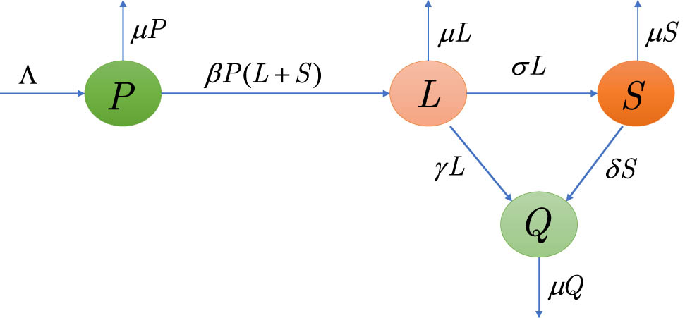
Flowchart of system (1).
Let
3 Threshold dynamics
3.1 Equilibria and basic reproduction number
The smoking-free equilibrium of system (1) is
By evaluating the Jacobian matrix of
Thus, the next-generation matrix is
Hence, the basic reproduction number of system (1) is given by
where
Let
According to (2) and (3), we have
3.2 Stability of the equilibria
Theorem 1
The smoking-free equilibrium
Proof
The Jacobian matrix of system (1) at
The characteristic equation of
where
If
Theorem 2
The smoking-present equilibrium
Proof
The Jacobian matrix of system (1) at
The characteristic equation of
where
Furthermore,
If
Theorem 3
The smoking-free equilibrium
Proof
Consider the following Lyapunov function:
The derivative of
Then
Theorem 4
The smoking-present equilibrium
Proof
Consider a Lyapunov function of the following form:
By calculating the derivative of
By using the fact that the geometric mean is less than or equal to the arithmetic mean, it can be deduced that
4 Numerical simulations and sensitivity analysis
4.1 Verification of theoretical results
This subsection aims to perform some numerical simulations to verify the dynamical behavior of system (1). Given an average lifespan of 70 years, the natural death rate is
First, let
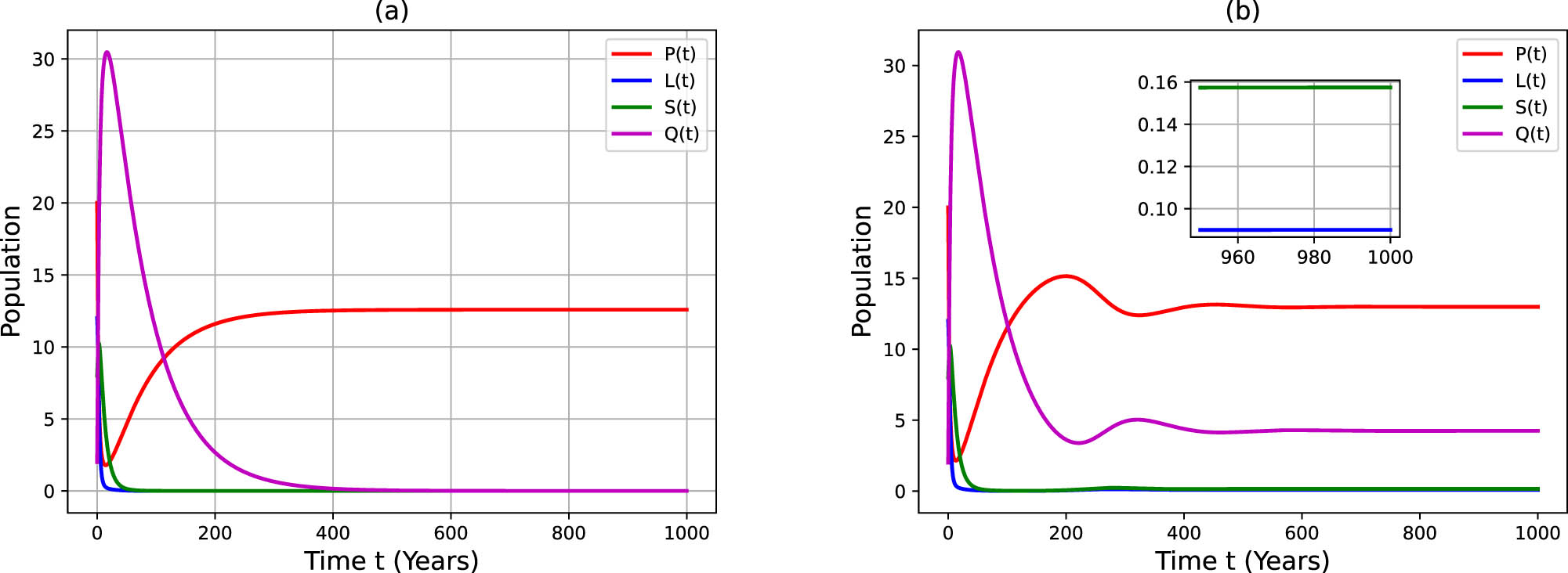
The plot shows the dynamical behavior of all classes for (a)
Then, let
4.2 Sensitivity analysis
4.2.1 Impact of parameters on
R
0
Understanding the transmission dynamics of smoking behavior in populations is crucial for controlling this public health epidemic. To design effective strategies for reducing smoking prevalence, we will use sensitivity analysis to assess how model parameters influence the basic reproduction number. It will reveal the key drivers of smoking’s persistence and transmission in communities.
The sensitivity index of
According to (2), the sensitivity indices of
Sensitivity indices of
| Parameter | Sensitivity index | Parameter | Sensitivity index |
|---|---|---|---|
|
|
1 |
|
1 |
|
|
|
|
0.3563403119 |
|
|
|
|
|
Therefore, the basic reproduction number
Furthermore, the contour plots of
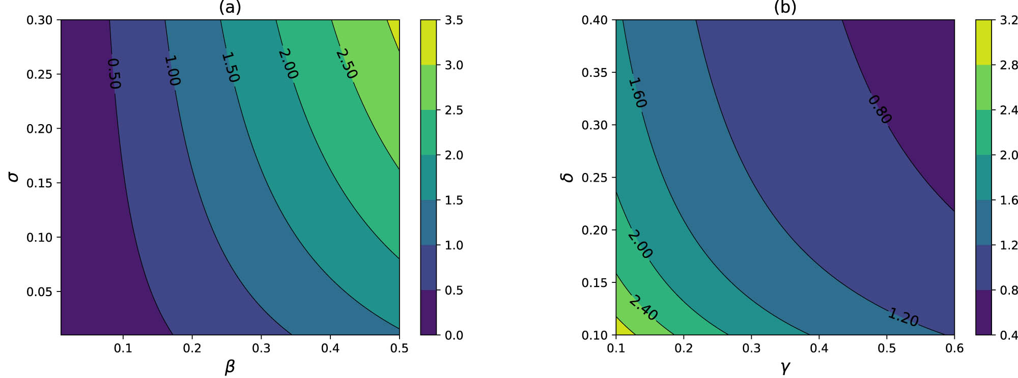
Contour plots of
4.2.2 Impact of parameters on the level of occasional and chain smokers
To further investigate the effect of parameters on the number of occasional and chain smokers,
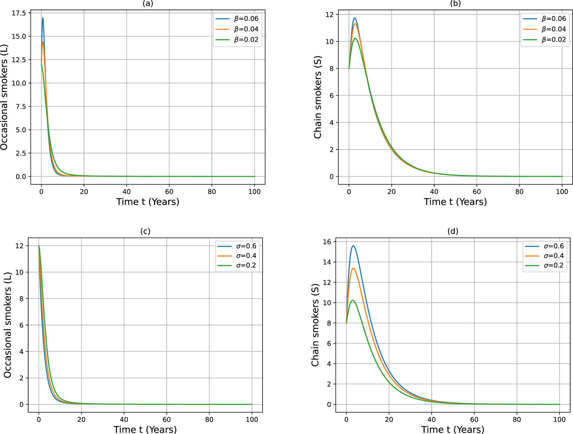
Impact of changes in
Figure 5 presents the influence of the quit rates
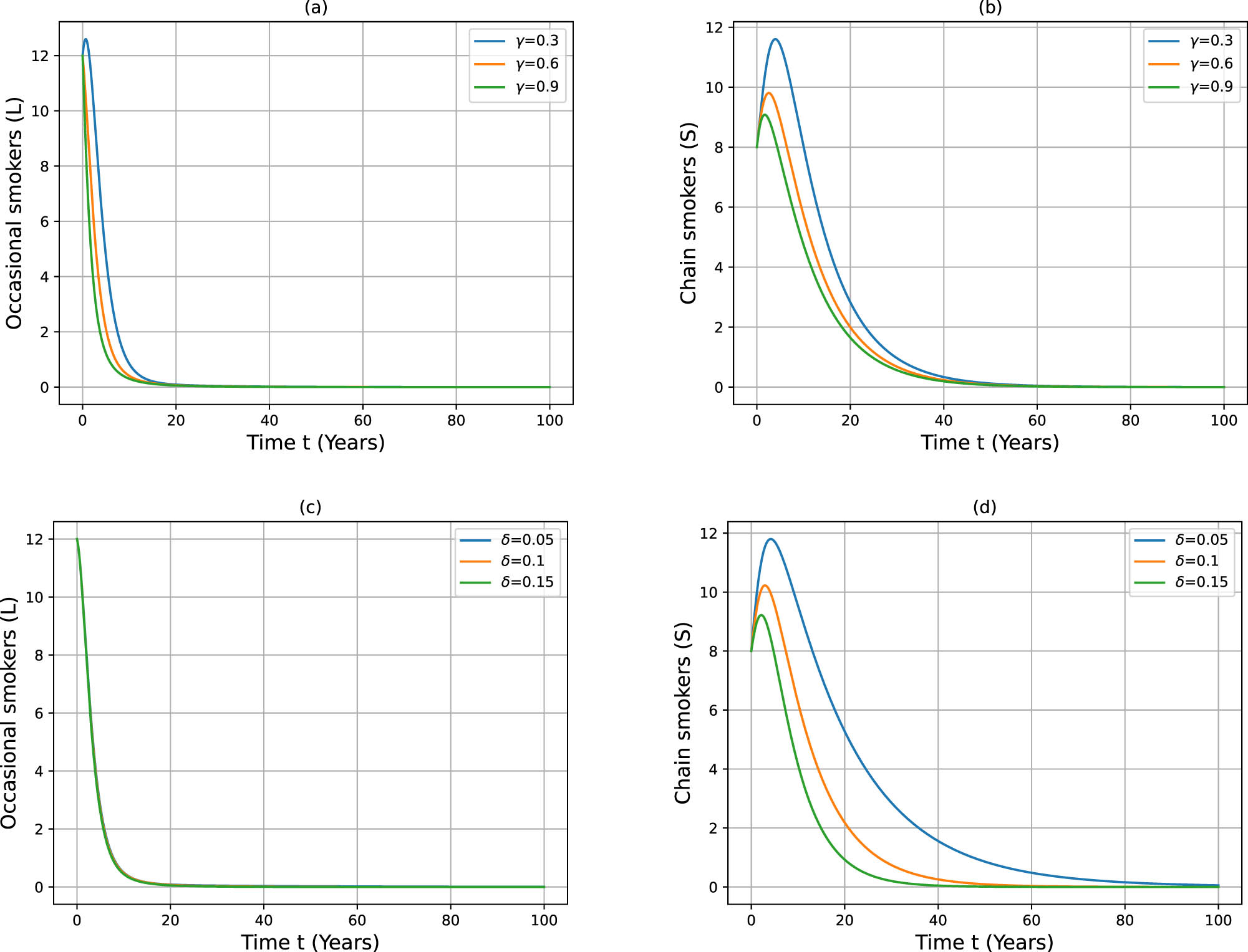
Impact of changes in
When smoking behavior can be eliminated, i.e.,
Completely banning smoking in large areas is unrealistic. Thus, when
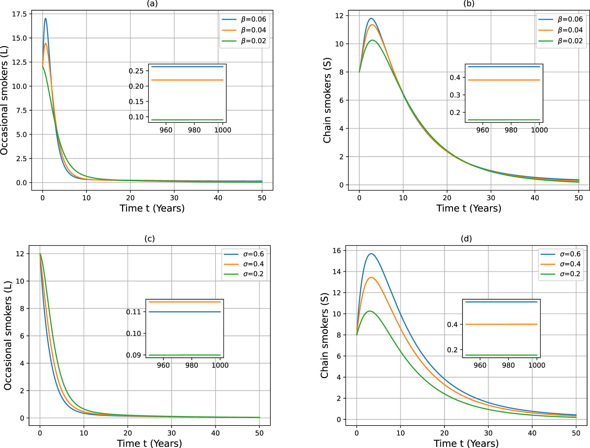
Impact of changes in
Figure 7 demonstrates how quit rates (
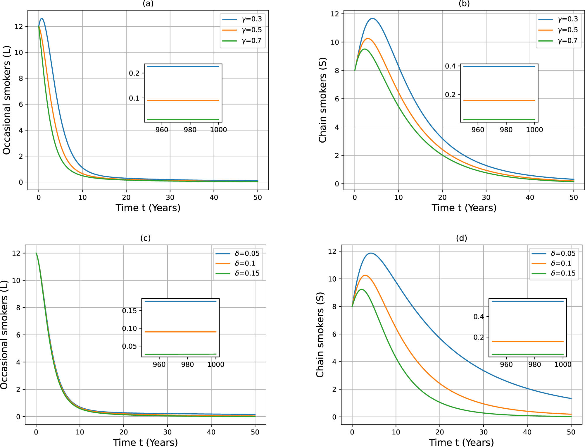
Impact of changes in
As shown in Figures 6 and 7, a decrease in the transmission rate (
5 Optimal control strategy
This section is dedicated to exploring the optimal control strategy of system (1). Sensitivity analysis has shown that the key to controlling smoking prevalence lies in the parameters
where
where
Pontryagin’s maximum principle [31] is employed to deduce the necessary conditions for determining the optimal controls
where
with boundary conditions
Now, the optimal control system (8–9) will be solved numerically. The weight constants are taken as
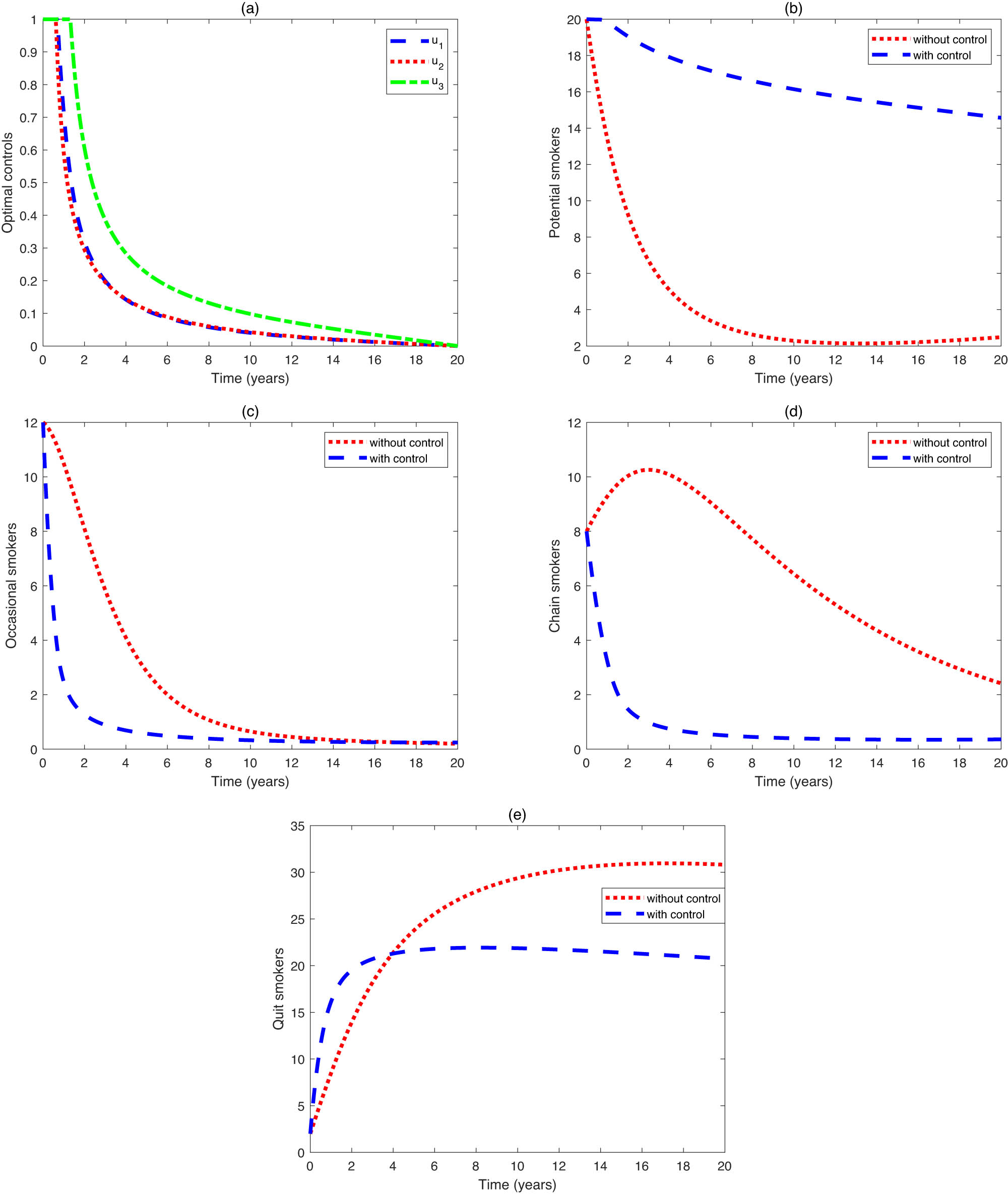
Controls applied to the population.
6 Conclusion
This article develops a potential-light-smoker-quit smoker smoking transmission model by incorporating the infection and quitting behaviors of occasional smokers. On the basis of the expression of
7 Discussion
Because neither the potential smoker recruitment rate nor the natural death rate can be practically adjusted, smoking control efforts must target the transmission, conversion, and quit rates. Therefore, to create smoke-free communities, policymakers should primarily focus on measures that impact the transmission rate and the quit rates of of smokers. Moreover, Figure 3 shows that the prevalence of smoking behavior can be efficiently controlled when the transmission rate
To control smoking prevalence, we propose three interventions: (i) creating smoke-free zones, (ii) implementing public health education about smoking risks, and (iii) providing treatment for nicotine dependence. These measures aim to reduce the number of smokers and ultimately eliminate smoking behavior. Figure 8 shows that the three control measures can achieve good results in tobacco control within 4 years. However, the number of potential smokers still exists and is increasing compared to the situation without control measures. Therefore, to prevent the resurgence of smoking, policymakers should also pay attention to how to reduce the number of potential smokers, such as by implementing periodic smoking hazard education campaigns.
Although this study is based on hypothetical data or values used in published articles, the same principles can be applied to communities where real data are available. Actually, relapse often occurs in ex-smokers due to stress, socialization, lack of will, etc. It is noticeable that in the smoking model (1), we do not take into account the relapse of quitters. We will consider this situation in future studies.
-
Funding information This work was supported by Sichuan Minzu College (No. XYZB2302ZA).
-
Author contributions: All authors have accepted responsibility for the entire content of this manuscript and approved its submission. Jianglin Zhao conceptualized, formulated, and analyzed the model. Lirong Ma reviewed the work.
-
Conflict of interest: The authors state no conflict of interest.
-
Data availability statement: All data generated or analysed during this study are included in this published article.
References
[1] Lin B, Liu X, Lu W, Wu X, Li Y, Zhang Z, et al. Prevalence and associated factors of smoking among chinese adolescents: a school-based cross-sectional study. BMC Public Health 2023;23:669. 10.1186/s12889-023-15565-3Suche in Google Scholar PubMed PubMed Central
[2] World Health Organization. Tobacco 2023. https://www.who.int/news-room/fact-sheets/detail/tobacco (accessed October 5, 2023). Suche in Google Scholar
[3] Zhang S, Meng Y, Chakraborty AK, Wang H. Controlling smoking: A smoking epidemic model with different smoking degrees in deterministic and stochastic environments. Math Biosci. 2024;368:109132. 10.1016/j.mbs.2023.109132Suche in Google Scholar PubMed
[4] Tan Y, Li X, Yang J, Cheke RA. Global stability of an age-structured model of smoking and its treatment. Int J Biomath 2023;16:2250063. 10.1142/S1793524522500632Suche in Google Scholar
[5] Naik PA, Yeolekar BM, Qureshi S, Manhas N, Ghoreishi M, Yeolekar M, et al. Global analysis of a fractional-order hepatitis B virus model under immune response in the presence of cytokines. Adv Theor Simul. 2024;7:2400726. 10.1002/adts.202400726Suche in Google Scholar
[6] Farman M, Hincal E, Naik PA, Hasan A, Sambas A, Nisar KS. A sustainable method for analyzing and studying the fractional-order panic spreading caused by the COVID-19 pandemic. Partial Differ Equ Appl Math. 2025;13:101047. 10.1016/j.padiff.2024.101047Suche in Google Scholar
[7] Naik PA, Farman M, Jamil K, Nisar KS, Hashmi MA, Huang Z. Modeling and analysis using piecewise hybrid fractional operator in time scale measure for ebola virus epidemics under Mittag-Leffler kernel. Sci Rep. 2024;14:24963. 10.1038/s41598-024-75644-2Suche in Google Scholar PubMed PubMed Central
[8] Naik PA, Yavuz M, Qureshi S, Naik M, Owolabi KM, Soomro A, et al. Memory impacts in hepatitis C: A global analysis of a fractional-order model with an effective treatment. Comput Methods Programs Biomed. 2024;254:108306. 10.1016/j.cmpb.2024.108306Suche in Google Scholar PubMed
[9] Naik PA, Yeolekar BM, Qureshi S, Yeolekar M, Madzvamuse A. Modeling and analysis of the fractional-order epidemic model to investigate mutual influence in HIV/HCV co-infection. Nonlinear Dyn. 2024;112:11679–710. 10.1007/s11071-024-09653-1Suche in Google Scholar
[10] Saleem MU, Farman M, Sarwar R, Naik PA, Abbass P, Hincal E, et al. Modeling and analysis of a carbon capturing system in forest plantations engineering with mittag-leffler positive invariant and global Mittag-Leffler properties. Model Earth Syst Environ. 2024;11:38. 10.1007/s40808-024-02181-2Suche in Google Scholar
[11] Jan R, Xiao Y. Effect of pulse vaccination on dynamics of dengue with periodic transmission functions. Adv Contin Discrete Models. 2019;2019:368. 10.1186/s13662-019-2314-ySuche in Google Scholar
[12] Jan R, Jan A. MSGDTM for solution of frictional order dengue disease model. Int J Sci Res. 2015;6:1139–44. Suche in Google Scholar
[13] Jan R, Boulaaras S, Alnegga M, Abdullah FA. Fractional-calculus analysis of the dynamics of typhoid fever with the effect of vaccination and carriers. Int J Numer Model El. 2024;37:e3184. 10.1002/jnm.3184Suche in Google Scholar
[14] Jan R, Razak NNA, Boulaaras S, Rehman ZU, Bahramand S. Mathematical analysis of the transmission dynamics of viral infection with effective control policies via fractional derivative. Nonlinear Eng Model. 2023;12:20220342. 10.1515/nleng-2022-0342Suche in Google Scholar
[15] Alshehri A, Shah Z, Jan R. Mathematical study of the dynamics of lymphatic filariasis infection via fractional-calculus. Eur Phys J Plus. 2023;138:280. 10.1140/epjp/s13360-023-03881-xSuche in Google Scholar PubMed PubMed Central
[16] Jan R, Hinçal E, Hosseini K, Razak NNA, Abdeljawad T, Osman MS. Fractional view analysis of the impact of vaccination on the dynamics of a viral infection. Alex Eng J. 2024;102:36–48. 10.1016/j.aej.2024.05.080Suche in Google Scholar
[17] Bahi MC, Bahramand S, Jan R, Boulaaras S, Ahmad H, Guefaifia R. Fractional view analysis of sexual transmitted human papilloma virus infection for public health. Sci Rep. 2024;14(1):3048. 10.1038/s41598-024-53696-8Suche in Google Scholar PubMed PubMed Central
[18] Deebani W, Jan R, Shah Z, Vrinceanu N, Racheriu M. Modeling the transmission phenomena of water-borne disease with non-singular and non-local kernel. Comput Methods Biomech Biomed Engin. 2023;26:1294–307. 10.1080/10255842.2022.2114793Suche in Google Scholar PubMed
[19] Jan R, Boulaaras S, Alyobi, Rajagopal K, Jawad M. Fractional dynamics of the transmission phenomena of dengue infection with vaccination. Discrete Cont Dyn-S. 2023;16(8):2096–117. 10.3934/dcdss.2022154Suche in Google Scholar
[20] Hussain T, Awan AU, Abro KA, Ozair M, Manzoor M. A mathematical and parametric study of epidemiological smoking model: a deterministic stability and optimality for solutions. Eur Phys J Plus. 2021;136:11. 10.1140/epjp/s13360-020-00979-4Suche in Google Scholar
[21] Harvim P, Zhang H, Georgescu P, Zhang L. Cigarette smoking on college campuses: an epidemical modelling approach. J Appl Math Comput. 2021;65:515–40. 10.1007/s12190-020-01402-ySuche in Google Scholar
[22] Khan H, Alzabut J, Gómez-Aguilar JF, Alkhazan A. Essential criteria for existence of solution of a modified-ABC fractional order smoking model. Ain Shams Eng J. 2024;15(5):102646. 10.1016/j.asej.2024.102646Suche in Google Scholar
[23] Madhusudanan V, Srinivas MN, Murthy BSN, Ansari KJ, Zeb A, Althobaiti A, et al. The influence of time delay and Gaussian white noise on the dynamics of tobacco smoking model. Chaos Soliton Fract. 2023;173:113616. 10.1016/j.chaos.2023.113616Suche in Google Scholar
[24] Rahman G, Agarwal RP, Liu L, Khan A. Threshold dynamics and optimal control of an age-structured giving up smoking model. Nonlinear Anal-Real. 2018;43:96–120. 10.1016/j.nonrwa.2018.02.006Suche in Google Scholar
[25] Zaman G. Qualitative behavior of giving up smoking model. B Malays Math Sci So. 2009;34:403–15. Suche in Google Scholar
[26] Zeb A, Zaman G, Momani S. Square-root dynamics of a giving up smoking model. Appl Math Model. 2013;37(7):5326–34. 10.1016/j.apm.2012.10.005Suche in Google Scholar
[27] Rahman G, Agarwal RP, Din Q. Mathematical analysis of giving up smoking model via harmonic mean type incidence rate. Appl Math Comput. 2019;354:128–48. 10.1016/j.amc.2019.01.053Suche in Google Scholar
[28] Sharomi O, Gumel AB. Curtailing smoking dynamics: A mathematical modeling approach. Appl Math Comput. 2008;195(2):475–99. 10.1016/j.amc.2007.05.012Suche in Google Scholar
[29] Guerrero F, Santonja F, Villanueva R. Analysing the Spanish smoke-free legislation of 2006: A new method to quantify its impact using a dynamic model. Int J Drug Policy. 2011;22(4):247–51. 10.1016/j.drugpo.2011.05.003Suche in Google Scholar PubMed
[30] Zhang Z, Ur Rahman G, Agarwal RP. Harmonic mean type dynamics of a delayed giving up smoking model and optimal control strategy via legislation. J Franklin Inst. 2020;357(15):10669–90. 10.1016/j.jfranklin.2020.09.002Suche in Google Scholar
[31] Lenhart S, Workman JT. Optimal control applied to biological models. 1st ed. New York: Chapman and Hall/CRC; 2007. 10.1201/9781420011418Suche in Google Scholar
© 2025 the author(s), published by De Gruyter
This work is licensed under the Creative Commons Attribution 4.0 International License.
Artikel in diesem Heft
- Research Articles
- Generalized (ψ,φ)-contraction to investigate Volterra integral inclusions and fractal fractional PDEs in super-metric space with numerical experiments
- Solitons in ultrasound imaging: Exploring applications and enhancements via the Westervelt equation
- Stochastic improved Simpson for solving nonlinear fractional-order systems using product integration rules
- Exploring dynamical features like bifurcation assessment, sensitivity visualization, and solitary wave solutions of the integrable Akbota equation
- Research on surface defect detection method and optimization of paper-plastic composite bag based on improved combined segmentation algorithm
- Impact the sulphur content in Iraqi crude oil on the mechanical properties and corrosion behaviour of carbon steel in various types of API 5L pipelines and ASTM 106 grade B
- Unravelling quiescent optical solitons: An exploration of the complex Ginzburg–Landau equation with nonlinear chromatic dispersion and self-phase modulation
- Perturbation-iteration approach for fractional-order logistic differential equations
- Variational formulations for the Euler and Navier–Stokes systems in fluid mechanics and related models
- Rotor response to unbalanced load and system performance considering variable bearing profile
- DeepFowl: Disease prediction from chicken excreta images using deep learning
- Channel flow of Ellis fluid due to cilia motion
- A case study of fractional-order varicella virus model to nonlinear dynamics strategy for control and prevalence
- Multi-point estimation weldment recognition and estimation of pose with data-driven robotics design
- Analysis of Hall current and nonuniform heating effects on magneto-convection between vertically aligned plates under the influence of electric and magnetic fields
- A comparative study on residual power series method and differential transform method through the time-fractional telegraph equation
- Insights from the nonlinear Schrödinger–Hirota equation with chromatic dispersion: Dynamics in fiber–optic communication
- Mathematical analysis of Jeffrey ferrofluid on stretching surface with the Darcy–Forchheimer model
- Exploring the interaction between lump, stripe and double-stripe, and periodic wave solutions of the Konopelchenko–Dubrovsky–Kaup–Kupershmidt system
- Computational investigation of tuberculosis and HIV/AIDS co-infection in fuzzy environment
- Signature verification by geometry and image processing
- Theoretical and numerical approach for quantifying sensitivity to system parameters of nonlinear systems
- Chaotic behaviors, stability, and solitary wave propagations of M-fractional LWE equation in magneto-electro-elastic circular rod
- Dynamic analysis and optimization of syphilis spread: Simulations, integrating treatment and public health interventions
- Visco-thermoelastic rectangular plate under uniform loading: A study of deflection
- Threshold dynamics and optimal control of an epidemiological smoking model
- Numerical computational model for an unsteady hybrid nanofluid flow in a porous medium past an MHD rotating sheet
- Regression prediction model of fabric brightness based on light and shadow reconstruction of layered images
- Dynamics and prevention of gemini virus infection in red chili crops studied with generalized fractional operator: Analysis and modeling
- Qualitative analysis on existence and stability of nonlinear fractional dynamic equations on time scales
- Fractional-order super-twisting sliding mode active disturbance rejection control for electro-hydraulic position servo systems
- Analytical exploration and parametric insights into optical solitons in magneto-optic waveguides: Advances in nonlinear dynamics for applied sciences
- Bifurcation dynamics and optical soliton structures in the nonlinear Schrödinger–Bopp–Podolsky system
- Review Article
- Haar wavelet collocation method for existence and numerical solutions of fourth-order integro-differential equations with bounded coefficients
- Special Issue: Nonlinear Analysis and Design of Communication Networks for IoT Applications - Part II
- Silicon-based all-optical wavelength converter for on-chip optical interconnection
- Research on a path-tracking control system of unmanned rollers based on an optimization algorithm and real-time feedback
- Analysis of the sports action recognition model based on the LSTM recurrent neural network
- Industrial robot trajectory error compensation based on enhanced transfer convolutional neural networks
- Research on IoT network performance prediction model of power grid warehouse based on nonlinear GA-BP neural network
- Interactive recommendation of social network communication between cities based on GNN and user preferences
- Application of improved P-BEM in time varying channel prediction in 5G high-speed mobile communication system
- Construction of a BIM smart building collaborative design model combining the Internet of Things
- Optimizing malicious website prediction: An advanced XGBoost-based machine learning model
- Economic operation analysis of the power grid combining communication network and distributed optimization algorithm
- Sports video temporal action detection technology based on an improved MSST algorithm
- Internet of things data security and privacy protection based on improved federated learning
- Enterprise power emission reduction technology based on the LSTM–SVM model
- Construction of multi-style face models based on artistic image generation algorithms
- Research and application of interactive digital twin monitoring system for photovoltaic power station based on global perception
- Special Issue: Decision and Control in Nonlinear Systems - Part II
- Animation video frame prediction based on ConvGRU fine-grained synthesis flow
- Application of GGNN inference propagation model for martial art intensity evaluation
- Benefit evaluation of building energy-saving renovation projects based on BWM weighting method
- Deep neural network application in real-time economic dispatch and frequency control of microgrids
- Real-time force/position control of soft growing robots: A data-driven model predictive approach
- Mechanical product design and manufacturing system based on CNN and server optimization algorithm
- Application of finite element analysis in the formal analysis of ancient architectural plaque section
- Research on territorial spatial planning based on data mining and geographic information visualization
- Fault diagnosis of agricultural sprinkler irrigation machinery equipment based on machine vision
- Closure technology of large span steel truss arch bridge with temporarily fixed edge supports
- Intelligent accounting question-answering robot based on a large language model and knowledge graph
- Analysis of manufacturing and retailer blockchain decision based on resource recyclability
- Flexible manufacturing workshop mechanical processing and product scheduling algorithm based on MES
- Exploration of indoor environment perception and design model based on virtual reality technology
- Tennis automatic ball-picking robot based on image object detection and positioning technology
- A new CNN deep learning model for computer-intelligent color matching
- Design of AR-based general computer technology experiment demonstration platform
- Indoor environment monitoring method based on the fusion of audio recognition and video patrol features
- Health condition prediction method of the computer numerical control machine tool parts by ensembling digital twins and improved LSTM networks
- Establishment of a green degree evaluation model for wall materials based on lifecycle
- Quantitative evaluation of college music teaching pronunciation based on nonlinear feature extraction
- Multi-index nonlinear robust virtual synchronous generator control method for microgrid inverters
- Manufacturing engineering production line scheduling management technology integrating availability constraints and heuristic rules
- Analysis of digital intelligent financial audit system based on improved BiLSTM neural network
- Attention community discovery model applied to complex network information analysis
- A neural collaborative filtering recommendation algorithm based on attention mechanism and contrastive learning
- Rehabilitation training method for motor dysfunction based on video stream matching
- Research on façade design for cold-region buildings based on artificial neural networks and parametric modeling techniques
- Intelligent implementation of muscle strain identification algorithm in Mi health exercise induced waist muscle strain
- Optimization design of urban rainwater and flood drainage system based on SWMM
- Improved GA for construction progress and cost management in construction projects
- Evaluation and prediction of SVM parameters in engineering cost based on random forest hybrid optimization
- Museum intelligent warning system based on wireless data module
- Optimization design and research of mechatronics based on torque motor control algorithm
- Special Issue: Nonlinear Engineering’s significance in Materials Science
- Experimental research on the degradation of chemical industrial wastewater by combined hydrodynamic cavitation based on nonlinear dynamic model
- Study on low-cycle fatigue life of nickel-based superalloy GH4586 at various temperatures
- Some results of solutions to neutral stochastic functional operator-differential equations
- Ultrasonic cavitation did not occur in high-pressure CO2 liquid
- Research on the performance of a novel type of cemented filler material for coal mine opening and filling
- Testing of recycled fine aggregate concrete’s mechanical properties using recycled fine aggregate concrete and research on technology for highway construction
- A modified fuzzy TOPSIS approach for the condition assessment of existing bridges
- Nonlinear structural and vibration analysis of straddle monorail pantograph under random excitations
- Achieving high efficiency and stability in blue OLEDs: Role of wide-gap hosts and emitter interactions
- Construction of teaching quality evaluation model of online dance teaching course based on improved PSO-BPNN
- Enhanced electrical conductivity and electromagnetic shielding properties of multi-component polymer/graphite nanocomposites prepared by solid-state shear milling
- Optimization of thermal characteristics of buried composite phase-change energy storage walls based on nonlinear engineering methods
- A higher-performance big data-based movie recommendation system
- Nonlinear impact of minimum wage on labor employment in China
- Nonlinear comprehensive evaluation method based on information entropy and discrimination optimization
- Application of numerical calculation methods in stability analysis of pile foundation under complex foundation conditions
- Research on the contribution of shale gas development and utilization in Sichuan Province to carbon peak based on the PSA process
- Characteristics of tight oil reservoirs and their impact on seepage flow from a nonlinear engineering perspective
- Nonlinear deformation decomposition and mode identification of plane structures via orthogonal theory
- Numerical simulation of damage mechanism in rock with cracks impacted by self-excited pulsed jet based on SPH-FEM coupling method: The perspective of nonlinear engineering and materials science
- Cross-scale modeling and collaborative optimization of ethanol-catalyzed coupling to produce C4 olefins: Nonlinear modeling and collaborative optimization strategies
- Unequal width T-node stress concentration factor analysis of stiffened rectangular steel pipe concrete
- Special Issue: Advances in Nonlinear Dynamics and Control
- Development of a cognitive blood glucose–insulin control strategy design for a nonlinear diabetic patient model
- Big data-based optimized model of building design in the context of rural revitalization
- Multi-UAV assisted air-to-ground data collection for ground sensors with unknown positions
- Design of urban and rural elderly care public areas integrating person-environment fit theory
- Application of lossless signal transmission technology in piano timbre recognition
- Application of improved GA in optimizing rural tourism routes
- Architectural animation generation system based on AL-GAN algorithm
- Advanced sentiment analysis in online shopping: Implementing LSTM models analyzing E-commerce user sentiments
- Intelligent recommendation algorithm for piano tracks based on the CNN model
- Visualization of large-scale user association feature data based on a nonlinear dimensionality reduction method
- Low-carbon economic optimization of microgrid clusters based on an energy interaction operation strategy
- Optimization effect of video data extraction and search based on Faster-RCNN hybrid model on intelligent information systems
- Construction of image segmentation system combining TC and swarm intelligence algorithm
- Particle swarm optimization and fuzzy C-means clustering algorithm for the adhesive layer defect detection
- Optimization of student learning status by instructional intervention decision-making techniques incorporating reinforcement learning
- Fuzzy model-based stabilization control and state estimation of nonlinear systems
- Optimization of distribution network scheduling based on BA and photovoltaic uncertainty
- Tai Chi movement segmentation and recognition on the grounds of multi-sensor data fusion and the DBSCAN algorithm
- Special Issue: Dynamic Engineering and Control Methods for the Nonlinear Systems - Part III
- Generalized numerical RKM method for solving sixth-order fractional partial differential equations