Generalized (ψ,φ)-contraction to investigate Volterra integral inclusions and fractal fractional PDEs in super-metric space with numerical experiments

Syed Khayyam Shah; Muhammad Sarwar; Manel Hleili; Mohammad Esmael Samei; Thabet Abdeljawad

doi:10.1515/nleng-2024-0032

Article Open Access

Generalized (ψ,φ)-contraction to investigate Volterra integral inclusions and fractal fractional PDEs in super-metric space with numerical experiments

Syed Khayyam Shah , Muhammad Sarwar , Manel Hleili , Mohammad Esmael Samei and Thabet Abdeljawad

Published/Copyright: February 10, 2025

Published by

Become an author with De Gruyter Brill

Submit Manuscript Author Information

From the journal Nonlinear Engineering Volume 14 Issue 1

Abstract

This article demonstrates the behavior of generalized ( ψ , φ )-type contraction mappings involving expressions of rational-type in the context of super-metric spaces. In this direction, we obtained unique and common fixed point results for a pair of mappings. The obtained results are then utilized to establish some corollaries. Moreover, numerical examples and applications related to the system of integral inclusions and fractal fractional partial differential equations have been presented to validate the established results. The central objective of this research is to provide a more comprehensive framework for generalizing classical results in the context of super-metric space.

Keywords: positive solution; fixed point; fractional differential equation; Riemann-Liouville fractional derivative; existence and uniqueness

MSC 2010: 34A08; 34A12; 34B15

1 Introduction

Integral inclusions and fractal fractional differential equations ( FDE s) have attracted the attention of researchers due to their utilization in many scientific fields. These mathematical structures are particularly significant because they allow for modeling complex phenomena that cannot be precisely described using classical differential equations. Integral inclusions benefit mathematical models, making them valid for systems with unknown or changing parameters, notably in control theory and optimization problems. FDE s, conversely, provide a framework to delineate the phenomena that exhibit anomalous diffusion or fractal characteristics commonly seen in disciplines like physics, biology, and finance. These mathematical constructs help analyze and describe mathematical dynamic systems in physics, engineering, biology, economics, etc. [1–7].

Integral inclusions help model dynamic systems properly because they can effectively describe the reasoning behind the processes. Particularly, integral inclusions of Volterra type

(1) ϶ ( x ) ∈ ∫ 0 x ⅁ ( x , u ) ℏ ( u , ϶ ( u ) ) d u + ζ ( x ) , x ∈ J ≔ [ 0 , λ ] , ζ ∈ C ( J ) ,

with non-empty compact values multivalued ℏ ∈ C ( J × R ) , ϶ → ℏ ( x , ϶ ) is lower semi-continuous for almost every x ∈ J , ⅁ ( x , u ) is measurable on [ 0 , x ] , for each x ∈ J , are widely applicable in many disciplines notably in modeling physical system, population dynamics, image processing, economics and finance, chemical and biomedical engineering [8,9].

Conversely, the introduction of the concept of fractal geometry into the equation of fractal fractional partial DE s ( FPDE s) provides a natural extension of the traditional FPDE s. This modification shows significant benefits in describing complex systems that exhibit irregular geometries and multi-scale capabilities [10–13]. Many processes are part of these systems. For example, flow through porous stuff, turbulent flow, and diffusion in varied environments. Fractal FPDE s provide a more comprehensive representation of natural systems’ intricate geometry and scale invariance

(2) D ϶ ♭ 0 FF y ( υ , ϶ ) = F ( υ , ϶ , y ( υ , ϶ ) ) , 0 < ♭ < 1 , y ( υ , 0 ) = 0 ,

where ( υ , ϶ ) ∈ J × [ 0 , £ ] , y ( υ , ϶ ) ∈ C ( V , R ) , V = J × [ 0 , £ ] , F is a continuous function and non-linear, i.e. F ( 0 , 0 , y ( 0 , 0 ) ) = 0 . Equations of this nature effectively represent the complex details and unchanging patterns in natural and artificial systems [14–18].

Fixed point theory (FPT) serves as a powerful tool in studying integral inclusions and fractal FPDE s. Solutions’ stability, uniqueness, and existence can be investigated using the theory of fixed points (FPs). The existence of FPs indicates links between integral inclusion/ PDE dynamics and the associated operators. The established FP results provided conditions that ensured distinct solutions. This link enables researchers to demonstrate the behavior of complex models such as integral inclusions and fractal FPDE s. Examining many diverse areas becomes trivial by combining integral inclusions, fractal FPDE s, and FPT. Multiple disciplines progressed because of this link. This is because they can shape flexible mathematical systems. These frameworks help us picture and comprehend intricate phenomena.

Furthermore, the concept of contraction has been expanded in several ways with regard to the domain of space. Karapinar and Khojasteh recently presented a new method to expand the metric structure, known as the super-metric space ( S -M-S) [19]. The study of S -M-S has garnered considerable attention in the disciplines of nonlinear analysis and FPT. In [20], Karapinar and Fulga presented a substantial foundation for investigating different contraction mappings and their corresponding characteristics. Similarly, Gourh et al. [21] discussed FP results via interpolation and rational contractions in the framework of super-metric spaces. In situations when ordinary metric spaces may not represent appropriate, S -M-Ss provide a valuable option due to their inherent flexibility.

This article presents the characteristics of generalized ( ψ , φ ) -type contractions in the context of S -M-S. These conceptual frameworks present novel opportunities for investigating the characteristics of mappings in S -M-Ss and offer a more comprehensive structure for generalizing classical results. The findings of this study hold substantial potential for future scholars in the fields of FPTs and nonlinear analysis. The results obtained from this research will significantly contribute to our understanding of the dynamics of mappings within versatile contexts.

2 Preliminaries

In 1969, Wong and Boyd [22] introduced a novel category of contractive mappings referred to as φ -contraction, which serves as a generalization of the Banach contraction principle. Moreover, the idea of weak φ -contraction was introduced by Alber and Guerre-Delabriere [23] in 1997, extending its application to Hilbert spaces. Nevertheless, Rhoades [24] has demonstrated that the findings of Alber and Guerre-Delabriere [23] remain applicable in entire metric spaces (M-S), as indicated below.

Theorem 2.1

[24] Consider a complete metric space ( X , d m ) , represent a mapping T : X → X and a non-decreasing, continuous function φ : [ 0 , ∞ ) → [ 0 , ∞ ) with φ ( 0 ) = 0 and φ ( x ) > 0 for every x > 0 . Then, T ensures a unique, FP, whenever

(3) d m ( T x , T y ) ⩽ d m ( x , y ) − φ ( d m ( x , y ) ) , ∀ x , y ∈ X .

Furthermore, Dutta and Choudhary [25] established the generalization of Theorem 2.1 as below.

Theorem 2.2

[25] Consider a complete M-S ( X , d m ) and a represent mapping T : X → X , a monotonic, non-decreasing, continuous function ψ : [ 0 , ∞ ) → [ 0 , ∞ ) with ψ ( x ) = 0 iff x = 0 and a lower semi-continuous function φ : [ 0 , ∞ ) → [ 0 , ∞ ) s.t φ ( x ) = 0 iff x = 0 . Then, T possesses a unique, FP, whenever

(4) ψ ( d m ( T x , T y ) ) ⩽ ψ ( d m ( x , y ) ) − φ ( d m ( x , y ) ) , ∀ x , y ∈ X .

Moreover, in 2009, Zhang and Song [26] obtained the below generalization of Theorem 2.1.

Theorem 2.3

[26] Suppose ( X , d m ) represent a complete M-S and suppose T , S : X → X represent two mappings. Let

(5) d m ( T x , S y ) ⩽ M ( T x , S y ) − φ ( M ( T x , S y ) ) , ∀ x , y ∈ X ,

whereas Theorem 2.2 defines φ and

(6) M ( x , y ) = max { d m ( x , y ) , d m ( x , T x ) , d m ( y , S y ) , d m ( y , T x ) + d m ( x , S y ) 2 .

Then, there must be a unique point x ∗ ∈ X s.t x ∗ = T x ∗ = S x ∗ .

Dorić [27] have established a similar common FP theorem for two mappings, further extending the findings as mentioned above.

Theorem 2.4

[27] Suppose ( X , d m ) represent a complete M-S and suppose T , S : X → X represent two mappings. Let

(7) ψ ( d m ( T x , S y ) ) ⩽ ψ ( M ( T x , S y ) ) − φ ( M ( T x , S y ) ) , ∀ x , y ∈ X ,

where Theorem 2.2 define ψ , φ , and (6). Then, there must be a unique point x ∗ ∈ X s.t. x ∗ = T x ∗ = S x ∗ .

Similarly, in 2017, He et al. [28] demonstrated the common FP theorem for two mappings that meet a generalized weak contractive-type condition of ( ψ , φ ) in complete M-S.

Theorem 2.5

[28] Suppose ( X , d m ) represent a complete M-S and T , S : X → X represent two mappings. Let for every x , y ∈ X , 1 2 min { d m ( x , T x ) , d m ( y , S y ) } ⩽ d m ( x , y ) implies

(8) ψ ( d m ( T x , S y ) ) ⩽ ψ ( M ( T x , S y ) ) − φ ( M ( T x , S y ) ) ,

whereas Theorem 2.2 defines ψ , φ , and (6). Then, there must be a unique point x ∗ ∈ X s.t x ∗ = T x ∗ = S x ∗ .

Currently, in 2020, the researchers [29] under a rational expression obtained the result below for the generalized ( ψ , φ ) -Suzuki weak contraction.

Theorem 2.6

[29] Suppose X represent a complete M-S and T : X → X represents a mapping. Let for every x , y ∈ X , 1 2 d m ( x , T x ) ⩽ d m ( x , y ) implies

(9) ψ ( d m ( T x , T y ) ) ⩽ ψ ( N ( T x , T y ) ) − φ ( N ( T x , T y ) ) ,

whereas Theorem 2.2 defines ψ , φ , and

(10) N ( x , y ) = max d m ( x , y ) , d m ( y , S y ) 1 + d m ( x , T x ) 1 + d m ( x , y ) .

Then, T has a unique FP.

Recently, Arya et al. [30] obtained two common FP results for mappings justifying the generalized ( ψ , φ ) -contractive-type conditions with a rational expression on a complete M-S.

Theorem 2.7

[30] Suppose X represent a complete M-S and suppose T , S : X → X represent two mappings. Let

(11) ψ ( d m ( T x , S y ) ) ⩽ ψ ( M 1 ( T x , S y ) ) − φ ( M 1 ( T x , S y ) ) , ∀ x , y ∈ X ,

whereas Theorem 2.2 defines ψ , φ , and

(12) M 1 ( x , y ) = max d m ( x , y ) , d m ( x , T x ) , d m ( y , S y ) , × d m ( y , T x ) + d m ( x , S y ) 2 , × d m ( x , T x ) + d m ( y , S y ) 2 , × d m ( y , S y ) 1 + d m ( x , T x ) 1 + d m ( x , y ) , × d m ( x , T x ) 1 + d m ( y , S x ) 1 + d m ( x , y ) .

Then, there exists a unique point x ∗ ∈ X s.t x ∗ = T x ∗ = S x ∗ .

Definition 2.8

[19] For a non-empty set Y , d s : Y × Y → [ 0 , + ∞ ) is termed as a super-metric if the following conditions hold

If d s ( ν , ω ) = 0 , then ν = ω for all ν , ω ∈ Y ;
d s ( ν , ω ) = d s ( ω , ν ) for all ν , ω ∈ Y ;
There we have s ⩾ 1 in a sense that for all ω ∈ Y , ∃ distinct sequences ( ν η ) , ( ω η ) ⊂ Y with d s ( ν η , ω η ) → 0 as η tends to infinity, s.t
(13) limsup η → ∞ d s ( ω n , ω ) ⩽ s limsup η → ∞ d s ( ν η , ω ) .

Then, we call ( Y , d s ) a S -M-S.

Example 2.9

[20] Suppose the set Y = [ 0 , + ∞ ] and d s : Y × Y → [ 0 , + ∞ ) represent an application, defined as follows:

(14) d s ( ν , ω ) = ∣ ν ω − 1 ∣ ν + ω + 1 , ν , ω ∈ [ 0 , 1 ) ∪ ( 1 , + ∞ ] , ν ≠ ω , 0 , ν , ω ∈ [ 0 , + ∞ ] , ν = ω , ∣ ν − 1 ∣ , ν ∈ [ 0 , + ∞ ] , ω = 1 .

Then, we can say ( Y , d s ) forms a S -M-S.

Example 2.10

[19] Suppose Y = [ 2 , 3 ] and define d s ( ν , ω ) = ν ω whenever ν ≠ ω and d s ( ν , ω ) = 0 whenever ν = ω . Suppose ( ν η ) , ( ω η ) be two distinct sequences s.t d s ( ν η , ω η ) → 0 as η → ∞ . As we the sequences are distinct, d s ( ν η , ω η ) = ν η ω η → 0 . It can be chosen that ω η → 0 and ν η → t as η → ∞ , where t ∈ Y . Furthermore, for any ω ∈ Y ,

(15) limsup η → ∞ d s ( ω η , ω ) = limsup η → ∞ ω η ω = 0 ⩽ limsup η → ∞ , d s ( ν η , ω ) = limsup η → ∞ υ η ω = t ⋅ ω ,

so, ( Y , d s ) is a S -M-S.

For this sequel, the concepts and notations listed below are essential. For a S -M-S ( Y , d s ) a sequence ( ν η ) in Y converges to ω in Y , iff d s ( υ η , ω ) tends to zero, as η goes to ∞ [19]. For a S -M-S ( Y , d s ) , a sequence ( ν η ) in Y can be claimed as a Cauchy sequence in Y , iff lim η → ∞ sup d s ( ν η , ν m ) : m > η = 0 [19]. A space ( Y , d s ) can be claimed as a complete super-metric space iff, every Cauchy sequence in Y converges [19].

3 Main results

This section will focus on establishing novel results of generalized ( ψ , φ ) -rational-type contractions in the framework of super-metric spaces.

Here is our first result in this direction.

Theorem 3.1

Consider a complete S -M-S, Y , and two mappings T , S : Y → Y . Let

(16) ψ ( d s ( T x , S y ) ) ⩽ ψ ( M 2 ( T x , S y ) ) − φ ( M 2 ( T x , S y ) ) , ∀ x , y ∈ Y ,

whereas Theorem 2.2 defines ψ , φ , and

(17) M 2 ( x , y ) = max d s ( x , y ) , d s ( x , T x ) , d s ( y , S y ) , d s ( x , T x ) + d s ( x , S y ) 2 , d s ( x , T y ) + d s ( y , S y ) 2 , d s ( y , S y ) 1 + d s ( x , T x ) 1 + d s ( x , y ) , d s ( x , T x ) 1 + d s ( y , S x ) 1 + d s ( x , y ) .

Then, there exists a unique point g ∗ ∈ Y s.t g ∗ = T g ∗ = S g ∗ .

Proof

Suppose y 0 ∈ Y is an arbitrary. Then, we can choose y 1 = S y 0 , y 2 = T y 1 , y 3 = S y 2 , and y 4 = T y 3 . In this way, a sequence can be constructed generally, y n in Y in a sense that y 2 n + 2 = T y 2 n + 1 and y 2 n + 1 = S y 2 n . Now, if x = y n and y = y n − 1 , for odd values of n , then by inequality (16), we have

(18) ψ ( d s ( T y n , S y n − 1 ) ) ⩽ ψ ( M 2 ( T y n , S y n − 1 ) ) − φ ( M 2 ( T y n , S y n − 1 ) ) ,

where

(19) M 2 ( T y n , S y n − 1 ) = max { d s ( y n , y n − 1 ) , d s ( y n , T y n ) , d s ( y n − 1 , S y n − 1 ) , d s ( y n , T y n ) + d s ( y n , S y n − 1 ) 2 , d s ( y n , T y n − 1 ) + d s ( y n − 1 , S y n − 1 ) 2 , d s ( y n − 1 , S y n − 1 ) 1 + d s ( y n , T y n ) 1 + d s ( y n , y n − 1 ) , d s ( y n , T y n ) 1 + d s ( y n − 1 , S y n ) 1 + d s ( y n , y n − 1 ) = max { d s ( y n , y n − 1 ) , d s ( y n , y n + 1 ) , d s ( y n − 1 , y n ) , d s ( y n , y n + 1 ) + d s ( y n , y n ) 2 , d s ( y n , y n ) + d s ( y n − 1 , y n ) 2 , d s ( y n − 1 , y n ) 1 + d s ( y n , y n + 1 ) 1 + d s ( y n , y n − 1 ) , d s ( y n , y n + 1 ) 1 + d s ( y n − 1 , y n + 1 ) 1 + d s ( y n , y n − 1 ) = d s ( y n , y n + 1 ) , d s ( y n − 1 , y n ) .

It implies that

(20) ψ ( d s ( y n + 1 , y n ) ) ⩽ ψ ( max { d s ( y n , y n + 1 ) , d s ( y n − 1 , y n ) } ) − φ ( max { d s ( y n , y n + 1 ) , d s ( y n − 1 , y n ) } ) .

If d s ( y n , y n + 1 ) > d s ( y n − 1 , y n ) , then inequality (20) can give

(21) ψ ( d s ( y n , y n + 1 ) ) ⩽ ψ ( d s ( y n , y n + 1 ) ) − φ ( d s ( y n , y n + 1 ) ) < ψ ( d s ( y n , y n + 1 ) ) ,

which is a contradiction. Hence, for all n , we obtain

(22) ψ ( d s ( y n , y n + 1 ) ) ⩽ ψ ( d s ( y n , y n − 1 ) ) − φ ( d s ( y n , y n − 1 ) ) .

Consequently, we have ψ ( d s ( y n , y n + 1 ) ) ⩽ ψ ( d s ( y n , y n − 1 ) ) . In analogue way, this inequality can be verified for those values of n which are even. Utilizing the property of ψ , for every n ∈ N , we have d s ( y n , y n + 1 ) ⩽ d s ( y n , y n − 1 ) . Moreover, the sequence { d s ( y n , y n + 1 ) } n ⩾ 1 is monotonic, non-increasing, and is bounded below, so there must be r ⩾ 0 in a sense that

(23) lim n → ∞ d s ( y n , y n + 1 ) = r = lim n → ∞ d s ( y n − 1 , y n ) .

Utilizing the lower semi-continuity of φ , we have

(24) φ ( r ) ⩽ liminf n → ∞ φ ( d s ( y n − 1 , y n ) ) .

Now, claiming r = 0 . Indeed, taking upper limit as n → ∞ on the below inequality and utilizing 23, we obtain

(25) ψ ( d s ( y n , y n + 1 ) ) ⩽ ψ ( d s ( y n − 1 , y n ) ) − φ ( d s ( y n − 1 , y n ) ) ⇒ ψ ( r ) ⩽ ψ ( r ) − φ ( r ) .

That is, φ ( r ) ⩽ 0 implies φ ( r ) = 0 , and φ ( r ) = 0 implies r = 0 . Hence, lim n → ∞ d s ( y n , y n + 1 ) = 0 . Now suppose that κ , n ∈ N and κ > n . If y n = y κ , we have T κ ( y 0 ) = T n ( y 0 ) . So, T κ − n ( T η ( y 0 ) ) = T η ( y 0 ) . Thus, T n ( y 0 ) is the FP of T κ − n . Also,

(26) T ( T κ − n ( T n ( y 0 ) ) ) = T κ − n ( T ( T n ( y 0 ) ) ) = T ( T n ( y 0 ) ) .

This means that T ( T n ( y 0 ) ) is the FP of T κ − n as well. Thus, T ( T n ( y 0 ) ) = T n ( y 0 ) . So T n ( y 0 ) is the FP of T . By following a similar approach for mapping S , S n ( y 0 ) is the FP of S . Now, maintaining generality, it can be supposed that, y n ≠ y κ . Therefore,

(27) limsup n → + ∞ d s ( y n , y n + 2 ) ⩽ limsup n → + ∞ d s ( y n + 1 , y n + 2 ) .

Thus, as limsup n → + ∞ d s ( y n , y n + 2 ) = 0 , we have

(28) limsup n → + ∞ d s ( y n , y n + 3 ) ⩽ limsup n → + ∞ d s ( y n + 2 , y n + 3 ) = 0 .

Inductively, it can be concluded that limsup n → + ∞ { d s ( y n , y κ ) : κ > n } = 0 . This leads to the fact that sequence { y n } is Cauchy. Provided with Y as a complete S -M-S, there must be g ∗ ∈ ℧ s.t y n → g ∗ . Next, we verify that g ∗ is the common FP of T and S . Utilizing (16), we have

(29) ψ ( d s ( T g ∗ , S y n ) ) ⩽ ψ ( M 2 ( T g ∗ , S y n ) ) − φ ( M 2 ( T g ∗ , S y n ) ) = ψ ( max { d s ( g ∗ , y n ) , d s ( g ∗ , T g ∗ ) , d s ( y n , S y n ) , d s ( g ∗ , T g ∗ ) + d s ( g ∗ , S y n ) 2 , d s ( g ∗ , T y n ) + d s ( y n , S y n ) 2 , − φ ( max { d s ( g ∗ , y n ) , d s ( g ∗ , T g ∗ ) , d s ( y n , S y n ) , d s ( g ∗ , T g ∗ ) + d s ( g ∗ , S y n ) 2 , d s ( g ∗ , T y n ) + d s ( y n , S y n ) 2 .

Making n → ∞ , we have ψ ( d s ( g ∗ , T g ∗ ) ) ⩽ ψ ( d s ( g ∗ , T g ∗ ) ) − φ ( d s ( g ∗ , T g ∗ ) ) , which yields g ∗ = T g ∗ . Furthermore, we obtain

(30) ψ ( d s ( T g ∗ , S g ∗ ) ) ⩽ ψ ( M 2 ( T g ∗ , S g ∗ ) ) − φ ( M 2 ( T g ∗ , S g ∗ ) ) = ψ ( max { d s ( g ∗ , g ∗ ) , d s ( g ∗ , T g ∗ ) , d s ( g ∗ , S g ∗ ) , d s ( g ∗ , T g ∗ ) + d s ( g ∗ , S g ∗ ) 2 , d s ( g ∗ , T g ∗ ) + d s ( g ∗ , S g ∗ ) 2 , − φ ( max { d s ( g ∗ , g ∗ ) , d s ( g ∗ , T g ∗ ) , d s ( g ∗ , S g ∗ ) , d s ( g ∗ , T g ∗ ) + d s ( g ∗ , S g ∗ ) 2 , d s ( g ∗ , T g ∗ ) + d s ( g ∗ , S g ∗ ) 2 .

It implies that ψ ( d s ( g ∗ , S g ∗ ) ) ⩽ ψ ( d s ( g ∗ , S g ∗ ) ) − φ ( d s ( g ∗ , S g ∗ ) ) , which yields g ∗ = S g ∗ . Hence, S and T have common FP g ∗ . To verify uniqueness, we assume that w is another FP of T and S , and we obtain

(31) ψ ( d s ( g ∗ , w ) ) = ψ ( d s ( T g ∗ , S w ) ) ⩽ ψ ( M 2 ( T g ∗ , S w ) ) − φ ( M 1 ( T g ∗ , S w ) ) = ψ ( d s ( g ∗ , w ) ) − φ ( d s ( g ∗ , w ) ) ,

and so φ ( d s ( w , g ∗ ) ) = 0 . Therefore, w = g ∗ . This completes the result.□

The above result can yield the following corollaries.

Corollary 3.2

Suppose Y represents a complete S -M-S and T , S : Y → Y represent two mappings. Let for every x , y ∈ Y ,

(32) d s ( T x , S y ) ⩽ M 2 ( T x , S y ) − φ ( M 2 ( T x , S y ) ) ,

whereas Theorem 2.2 defines ψ , φ , and (17). Then, there exists a unique point g ∈ Y s.t g = T g = S g .

Proof

The proof is quite simple by plugging ψ = I (Identity) in Theorem 3.1.□

Corollary 3.3

Suppose Y represents a complete S -M-S and T : Y → Y represents two mappings. Let for every x , y ∈ Y ,

(33) ψ ( d s ( T x , T y ) ) ⩽ ψ ( M 2 ( T x , T y ) ) − φ ( M 2 ( T x , T y ) ) ,

whereas Theorem 2.2 defines ψ and φ . Then, there exists a unique point g ∈ Y s.t g ∗ = T g ∗ .

Proof

Plugging S = T in Theorem 3.1, we will obtain the result.□

Corollary 3.4

Suppose Y represents a complete S -M-S and T : Y → Y represents s mappings. Let for every x , y ∈ Y ,

(34) d s ( T x , T y ) ⩽ M 2 ( T x , T y ) − φ ( M 2 ( T x , T y ) ) ,

whereas Theorem 2.2 defines ψ , φ , and (17). Then, there exists a unique point g ∗ ∈ Y s.t g ∗ = T g ∗ .

Proof

This can be proved simply by plugging S = T and taking ψ = I (Identity) in Theorem 3.1.□

Corollary 3.5

Suppose Y represent a complete S -M-S and T , S : Y → Y represent two mappings. Let for every x , y ∈ Y ,

(35) ψ ( d s ( T x , S y ) ) ⩽ ψ ( d s ( x , y ) ) − φ ( d s ( x , y ) ) ,

whereas Theorem 2.2 defines ψ and φ . Then there exists a unique point g ∗ ∈ Y s.t. g ∗ = T g ∗ = S g ∗ .

Proof

The proof is quite simple by plugging M 2 ( T x , S y ) = d ( x , y ) in Theorem 3.1.□

Corollary 3.6

Suppose Y represents a complete S -M-S and T : Y → Y represent two mappings. Let for every x , y ∈ Y ,

(36) d s ( T x , S y ) ⩽ ( d s ( x , y ) ) − φ ( d s ( x , y ) ) ,

whereas Theorem 2.2 define ψ and φ . Then there exists a unique point g ∈ Y s.t. g ∗ = T g ∗ = S g ∗ .

Proof

The proof is quite simple by plugging M 2 ( T x , S y ) = d ( x , y ) and ψ = I (Identity) in Theorem 3.1.□

Remark 3.7

The corollary 3.6 is the result (2.1) of [24] in the context of super-metric spaces.

Remark 3.8

The corollary 3.5 is the result (2.2) of [25] in the context of S -M-Ss.

Corollary 3.9

Suppose Y represent a complete S -M-S and T , S : Y → Y represent two mappings. Let for every x , y ∈ Y ,

(37) ψ ( d s ( T x , S y ) ) ⩽ ψ ( N ( T x , S y ) ) − φ ( N ( T x , S y ) ) ,

whereas Theorem 2.2 defines ψ , φ , and (10). Then there must be a unique point g ∗ ∈ Y in a sense that g ∗ = T g ∗ = S g ∗ .

Example 3.10

Suppose Y = [ 2 , 3 ] with super-metric be defined as

(38) d s ( x , y ) = x y , x ≠ y , 0 , x = y .

Now, consider T : Y → Y and S : Y → Y , as follows:

(39) T ( x ) = 2 , x ≠ 3 , 5 2 , x = 3 , S ( x ) = 1 , x ≠ 3 , 1 2 , x = 3 .

Then, proving the below is not tedious, for choosing ψ ( x ) = 2 x and φ ( x ) = x 7 ,

(40) ψ ( d s ( T x , S y ) ) ⩽ ψ ( M 2 ( T x , S y ) ) − φ ( M 2 ( T x , S y ) ) .

All the necessities of Theorem 3.1, Corollaries 3.5 and 3.9 are fulfilled. Thus, the FP of S and T is common and for sure would be unique.

Furthermore, following the same flow, we would like to prove a common FP theorem for the ( ψ , φ ) -rational contraction in the Suzuki-type context.

Theorem 3.11

Suppose Y represents a complete S -M-S and T , S : Y → Y represent two mappings. Let for every x , y ∈ Y , 1 2 min d s ( x , T x ) , d s ( y , S y ) ⩽ d s ( x , y ) and

(41) ψ ( d s ( T x , S y ) ) ⩽ ψ ( M 2 ( T x , S y ) ) − φ ( M 2 ( T x , S y ) ) ,

whereas Theorem 2.2 defines ψ , φ , and (17). Then, there exists a unique point g ∗ ∈ Y s.t g ∗ = T g ∗ = S g ∗ .

Proof

Suppose y 0 ∈ Y is an arbitrary. Then, a sequence y n in Y can be constructed in a way y 2 n − 1 = T y 2 n − 2 and y 2 n = S y 2 n − 1 . The below fact will be considered in this sequel, 1 2 min d s ( x , T x ) , d s ( y , S y ) ⩽ d s ( x , y ) iff d s ( x , T x ) ⩽ d s ( x , y ) and d s ( y , S y ) ⩽ d s ( x , y ) . If for some n y n = y n − 1 , then a common FP must be represented. The reason is if we consider y 2 n = y 2 n − 1 , then y 2 n − 1 is a common FP of the mappings. Indeed, utilizing Eq. (41)

(42) 1 2 d s ( y 2 n − 1 , S y 2 n − 1 ) = 1 2 d s ( y 2 n − 1 , y 2 n ) = 0 ⩽ d s ( y 2 n , y 2 n − 1 ) ,

implies

(43) ψ ( d s ( T y 2 n , S y 2 n − 1 ) ) ⩽ ψ ( M 1 ( T y 2 n , S y 2 n − 1 ) ) − φ ( M 1 ( T y 2 n , S y 2 n − 1 ) ) ,

where M 1 ( T y 2 n , S y 2 n − 1 ) = d s ( y 2 n , y 2 n + 1 ) = d s ( y 2 n , T y 2 n ) . Then, we have

(44) ψ ( d s ( T y 2 n , y 2 n ) ) ⩽ ψ ( d s ( T y 2 n , y 2 n ) ) − φ ( d s ( T y 2 n , y 2 n ) ) ,

which implies φ ( d s ( T y 2 n , y 2 n ) ) ⩽ 0 . Using the property of φ , we obtain T y 2 n = y 2 n . Thus, by S y 2 n − 1 = y 2 n = y 2 n − 1 , it implies that S y 2 n − 1 = y 2 n − 1 = T y 2 n − 1 , i.e., y 2 n − 1 is a common FP of T and S . In the same way, if y 2 n − 1 = y 2 n − 2 for some n , then y 2 n − 2 is a common FP of T and S . Thus, we suppose that y n ≠ y n − 1 for all n ∈ N . Observe that, all n ∈ N , have

(45) 1 2 d s ( y 2 n − 1 , S y 2 n − 1 ) = 1 2 d s ( y 2 n − 1 , y 2 n ) ⩽ d s ( y 2 n , y 2 n − 1 ) .

Then, by (41),

(46) ψ ( d s ( T y 2 n , S y 2 n − 1 ) ) ⩽ ψ ( M 1 ( T y 2 n , S y 2 n − 1 ) ) − φ ( M 1 ( T y 2 n , S y 2 n − 1 ) ) ,

where

(47) M 1 ( T y 2 n , S y 2 n − 1 ) = max { d s ( y 2 n , y 2 n − 1 ) , d s ( y 2 n , y 2 n + 1 ) } .

If M 1 ( T y 2 n , S y 2 n − 1 ) = d s ( y 2 n , y 2 n + 1 ) , then (46) becomes

(48) ψ ( d s ( y 2 n , y 2 n + 1 ) ) ⩽ ψ ( d s ( y 2 n , y 2 n + 1 ) ) − φ ( d s ( y 2 n , y 2 n + 1 ) ) ,

which implies φ ( d s ( y 2 n , y 2 n + 1 ) ) ⩽ 0 and so d s ( y 2 n , y 2 n + 1 ) = 0 . This led to a contradiction to our assumption y n ≠ y n − 1 . As a result (46) becomes

(49) ψ ( d s ( y 2 n , y 2 n + 1 ) ) ⩽ ψ ( d s ( y 2 n , y 2 n − 1 ) ) − φ ( d s ( y 2 n , y 2 n − 1 ) ) .

Similarly, we can find that

(50) ψ ( d s ( y 2 n + 1 , y 2 n + 2 ) ) ⩽ ψ ( d s ( y 2 n , y 2 n + 1 ) ) − φ ( d s ( y 2 n , y 2 n + 1 ) ) .

Now, combining Eqs. (49) and (50)

(51) ψ ( d s ( y n , y n + 1 ) ) ⩽ ψ ( d s ( y n , y n − 1 ) ) − φ ( d s ( y n , y n − 1 ) )

for all n ∈ N . Since φ ( d s ( y n , y n − 1 ) ) > 0 , we have ψ ( d s ( y n + 1 , y n ) ) < ψ ( d s ( y n , y n − 1 ) ) . Utilizing the property of ψ , for all n ∈ N , we have d s ( y n + 1 , y n ) < d s ( y n , y n − 1 ) . Moreover, the sequence { d s ( y n , y n + 1 ) } n = 0 ∞ is non-increasing, monotonic, and bounded below, and so there exists r ⩾ 0 in a sense that

(52) lim n → ∞ d s ( y n , y n + 1 ) = r = lim n → ∞ d s ( y n − 1 , y n ) .

Utilizing the lower semi-continuity of φ , we have φ ( r ) ⩽ liminf n → ∞ φ ( d s ( y n − 1 , y n ) ) . Now, we claim that r = 0 . Indeed, taking upper limit as n → ∞ on the following inequality and using (52), we obtain

(53) ψ ( d s ( y n , y n + 1 ) ) ⩽ ψ ( d s ( y n − 1 , y n ) ) − φ ( d s ( y n − 1 , y n ) ) ⇒ ψ ( r ) ⩽ ψ ( r ) − φ ( r ) .

That is, φ ( r ) ⩽ 0 implies φ ( r ) = 0 , and φ ( r ) = 0 implies r = 0 . Hence, lim n → ∞ d s ( y n , y n + 1 ) = 0 . Now, suppose that κ , n ∈ N and κ > n . If y n = y κ , we have T κ ( y 0 ) = T n ( y 0 ) . Indeed, T κ − n ( T η ( y 0 ) ) = T η ( y 0 ) . Thus, T n ( y 0 ) is the FP of T κ − n . Also,

(54) T ( T κ − n ( T n ( y 0 ) ) ) = T κ − n ( T ( T n ( y 0 ) ) ) = T ( T n ( y 0 ) ) .

This means that T ( T n ( y 0 ) ) is the FP of T κ − n as well. Thus, T ( T n ( y 0 ) ) = T n ( y 0 ) . So T n ( y 0 ) is the FP of T . By following similar approach for mapping S , S n ( y 0 ) is the FP of S . Now, maintaining generality, it can be supposed that, y n ≠ y κ . Therefore, limsup n → + ∞ d s ( y n , y n + 2 ) ⩽ limsup n → + ∞ d s ( y n + 1 , y n + 2 ) . Thus, as limsup n → + ∞ d s ( y n , y n + 2 ) = 0 . We have

(55) limsup n → + ∞ d s ( y n , y n + 3 ) ⩽ limsup n → + ∞ d s ( y n + 2 , y n + 3 ) = 0 .

Inductively, it can be concluded that limsup n → + ∞ { d s ( y n , y κ ) : κ > n } = 0 . This leads to the fact that sequence { y n } is Cauchy. Provided with Y as a complete S -M-S, there must be a g ∗ ∈ Y s.t y n → g ∗ . Next, we want to verify that g ∗ is the common FP of T and S . Utilizing (41), we have

(56) ψ ( d s ( T g ∗ , S y n ) ) ⩽ ψ ( M 2 ( T g ∗ , S y n ) ) − φ ( M 2 ( T g ∗ , S y n ) ) = ψ ( max { d s ( g ∗ , y n ) , d s ( g ∗ , T g ∗ ) , d s ( y n , S y n ) , d s ( g ∗ , T g ∗ ) + d s ( g ∗ , S y n ) 2 , d s ( g ∗ , T y n ) + d s ( y n , S y n ) 2 , − φ ( max { d s ( g ∗ , y n ) , d s ( g ∗ , T g ∗ ) , d s ( y n , S y n ) , d s ( g ∗ , T g ∗ ) + d s ( g ∗ , S y n ) 2 , d s ( g ∗ , T y n ) + d s ( y n , S y n ) 2 .

Making n → ∞ , we have ψ ( d s ( g ∗ , T g ∗ ) ) ⩽ ψ ( d s ( g ∗ , T g ∗ ) ) − φ ( d s ( g ∗ , T g ∗ ) ) , which yields g ∗ = T g ∗ . Furthermore, we obtain

(57) ψ ( d s ( T g ∗ , S g ∗ ) ) ⩽ ψ ( M 2 ( T g ∗ , S g ∗ ) ) − φ ( M 2 ( T g ∗ , S g ∗ ) ) = ψ ( max { d s ( g ∗ , g ∗ ) , d s ( g ∗ , T g ∗ ) , d s ( g ∗ , S g ∗ ) , d s ( g ∗ , T g ∗ ) + d s ( g ∗ , S g ∗ ) 2 , d s ( g ∗ , T g ∗ ) + d s ( g ∗ , S g ∗ ) 2 , − φ ( max { d s ( g ∗ , g ∗ ) , d s ( g ∗ , T g ∗ ) , d s ( g ∗ , S g ∗ ) , d s ( g ∗ , T g ∗ ) + d s ( g ∗ , S g ∗ ) 2 , d s ( g ∗ , T g ∗ ) + d s ( g ∗ , S g ∗ ) 2 .

It implies that ψ ( d s ( g ∗ , S g ∗ ) ) ⩽ ψ ( d s ( g ∗ , S g ∗ ) ) − φ ( d s ( g ∗ , S g ∗ ) ) , which yields g ∗ = S g ∗ . Hence, the mappings S and T have common FP g ∗ . To verify the uniqueness, assume that w is another FP of T and S , and we obtain

(58) ψ ( d s ( g ∗ , w ) ) = ψ ( d s ( T g ∗ , S w ) ) ⩽ ψ ( M 2 ( T g ∗ , S w ) ) − φ ( M 1 ( T g ∗ , S w ) ) = ψ ( d s ( g ∗ , w ) ) − φ ( d s ( g ∗ , w ) ) ,

and so φ ( d s ( w , g ∗ ) ) = 0 . Therefore, w = g ∗ . This completes the proof.□

The above result (3.11) yields the following corollaries. If S = T in the above result, we have the below corollary.

Corollary 3.12

Suppose Y represents a complete S -M-S and T : Y → Y represents a mappings. Let for every x , y ∈ Y , 1 2 min { d s ( x , T x ) , d s ( y , T y ) } ⩽ d s ( x , y ) and

(59) ψ ( d s ( T x , T y ) ) ⩽ ψ ( M 2 ( T x , T y ) ) − φ ( M 2 ( T x , T y ) ) ,

whereas Theorem 2.2 defines ψ , φ and (17). Then, there exists a unique element g ∗ ∈ Y s.t. g ∗ = T g ∗ .

Putting ψ = I (Identity) in (3.11), we have the following corollary.

Corollary 3.13

Suppose Y represent a complete S -M-S and T , S : Y → Y represent two mappings. Let for every x , y ∈ Y , 1 2 min { d s ( x , T x ) , d s ( y , S y ) } ⩽ d s ( x , y ) and

(60) d s ( T x , S y ) ⩽ M 2 ( T x , S y ) − φ ( M 2 ( T x , S y ) ) ,

whereas Theorem 2.2 defines ψ , φ , and (17). Then, there exists a unique element g ∗ ∈ Y s.t g ∗ = T g ∗ = S g ∗ .

4 Applications

In the following sections, we demonstrate the practical applications of the established findings. These applications aim to examine the validity of the established findings and offer assurance of the existence of common and unique solutions for integral inclusions of the Volterra type, as well as solutions for nonlinear DE s involving fractal fractional operators. The applications presented in this study serve to illustrate the practical importance and resilience of the theoretical findings, hence highlighting their use in the modeling and analysis of intricate dynamic systems characterized by memory effects and non-local interactions. The description of these applications strengthens the validity of the built theoretical framework and highlights its usefulness in tackling practical issues in various scientific fields.

4.1 Application to Volterra integral inclusions

In this subsection, the existence of a solution to the system of Volterra integral inclusions is demonstrated in the frame work of super-metric space. Motivated by the works of [1,3] an existence result demonstrating the existence of the system of Volterra integral inclusions has been presented

(61) ϶ 1 ( x ) ∈ ∫ 0 x ⅁ 1 ( x , u ) ℏ 1 ( u , ϶ 1 ( u ) ) d u + ζ ( x ) , ϶ 2 ( x ) ∈ ∫ 0 x ⅁ 2 ( x , u ) ℏ 2 ( u , ϶ 2 ( u ) ) d u + ζ ( x ) ,

for x ∈ J , ζ ∈ C ( J ) where multivalued ℏ 1 , ℏ 2 ∈ C ( J × R ) have non-empty compact values. Throughout this section, the map ϶ → ℏ i ( x , ϶ ) , i = 1 , 2 , is lower semi-continuous at x ∈ J . Define a super-metric d s : Y × Y → Y by

(62) d s ( ϶ 1 , ϶ 2 ) = ϶ 1 ⋅ ϶ 2 ϶ 1 ≠ ϶ 2 , 0 , ϶ 1 = ϶ 2 .

Next, we present the proof as follows.

Theorem 4.1

Suppose that, for all ϶ , w ∈ C ( J ) , the following conditions hold:

There exists a continuous function ℏ 1 , ℏ 2 ∈ J × R s.t.
(63) ∣ ℏ 1 ( x , ϶ 1 ( u ) ) ⋅ ℏ 2 ( x , ϶ 2 ( u ) ) ∣ ⩽ ∣ M 2 ( ϶ 1 ( u ) , ϶ 2 ( u ) ) − φ ( M 2 ( ϶ 1 ( u ) , ϶ 2 ( u ) ) ) ∣ ,
where M 2 is obtained by substituting d in (17);
There exist x , u ∈ J and τ > 0 s.t.
(64) ∫ 0 x ⅁ 1 ( x , u ) d u ⋅ ∫ 0 x ⅁ 2 ( x , u ) d u ⩽ 1 , ζ ( τ ) = 0 .
φ and ψ are defined in Theorem 2.2.

Then, the system of Volterra integral inclusions (61) have a unique solution.

Proof

Using the Volterra integral inclusion (61), we can define two operators S , T : Y → Y as follows:

(65) T ϶ ( x ) ∈ ∫ 0 x ⅁ 1 ( x , u ) ℏ 1 ( u , ϶ ( u ) ) d u + ζ ( x ) , S ϶ ( x ) ∈ ∫ 0 x ⅁ 2 ( x , u ) ℏ 2 ( u , ϶ ( u ) ) d u + ζ ( x ) ,

for x ∈ J , ζ ∈ Y , which implies that ϶ is the common and unique FP of the operator T and S , if and only if it is a solution of Eq. (61). Now, for all ϶ 1 , ϶ 2 ∈ Y , using conditions (6), (10), and (65), we obtain

(66) d s ( T ϶ 1 , S ϶ 2 ) = ∫ J ⅁ 1 ( x , u ) ∣ ℏ 1 ( u , ϶ 1 ( u ) ) ∣ d u ⋅ ∫ J ⅁ 2 ( x , u ) ∣ ℏ 2 ( u , ϶ 2 ( u ) ) ∣ d u = ∫ J ⅁ 1 ( x , u ) d u ⋅ ∫ J ⅁ 2 ( x , u ) d u ∣ ℏ 1 ( u , ϶ 1 ( u ) ) ℏ 2 ( u , ϶ 2 ( u ) ) ∣ ⩽ M 2 ( ϶ 1 ( u ) , ϶ 2 ( u ) ) − φ ( M 2 ( ϶ 1 ( u ) , ϶ 2 ( u ) ) .

Now, by taking ψ ( x ) = x ,

(67) ψ ( d s ( T ϶ 1 , S ϶ 2 ) ) ⩽ ψ ( M 2 ( ϶ 1 ( u ) , ϶ 2 ( u ) ) ) − φ ( M 2 ( ϶ 1 ( u ) , ϶ 2 ( u ) ) ) .

Hence, by Theorem 3.1, a ∗ is the unique and common FP of S and T . Thus, (65) has a unique solution, which is also a solution of the Volterra integral inclusion (61). This completes our proof.□

4.2 Application to fractal FPDE s

In this section, we established existence results for investigation of the unique theoretical solution for general PDE s involving fractal fractional derivative operators in the context of S -M-S:

(68) D ϶ ♭ 0 FF y ( υ , ϶ ) = F ( υ , ϶ , y ( υ , ϶ ) ) , 0 < ♭ < 1 , y ( υ , 0 ) = 0 ,

where ( υ , ϶ ) ∈ J × [ 0 , £ ] , y ( υ , ϶ ) ∈ C ( V , R ) , V = J × [ 0 , £ ] , F is a function continuous and non-linear, i.e. F ( 0 , 0 , y ( 0 , 0 ) ) = 0 . Let us consider Y = C ( V , R ) and d ( y , ω ) = ∣ y ( υ ) ⋅ ω ( ϶ ) ‖ , for y ≠ ω .

Theorem 4.2

Let us assume that the following holds in a way that:

for ( υ , ϶ ) ∈ J and y ( υ , ϶ ) , ω ( υ , ϶ ) ∈ Y ,
(69) ∣ F ( υ , ϶ , y ( υ , ϶ ) ) ⋅ F ( υ , ϶ , ω ( υ , ϶ ) ) ∣ ⩽ ς ♭ 2 ♭ ⊤ 2 ♭ − 1 ℬ ( ♭ , ♭ ) ∣ M 2 ( y ( υ , ϶ ) ω ( υ , ϶ ) ∣ ) − φ ( ∣ M 2 ( y ( υ , ϶ ) ω ( υ , ϶ ) ∣ ) ) ,
with d ( y , ω ) ⩾ 0 ; where ψ and φ are defined as in Theorem 2.2;
There exists y 1 ∈ Y with d ( y , T y 1 ) ⩾ 0 , where T : C → C defined as
(70) T ( y ) = 1 ς ( ♭ ) ∫ 0 t ♭ ⋎ ♭ − 1 ( ϶ − ⋎ ) ♭ − 1 F ( υ , ⋎ , y 1 ( υ , ⋎ ) ) d ⋎ ;
∫ 0 ∍ ∫ 0 ∍ ( ⋎ ♭ − 1 ( ϶ − ⋎ ) ♭ − 1 ) 2 d ⋎ d ⋎ ⩽ ⊤ 2 ♭ − 1 ℬ ( ♭ , ♭ ) and ( υ , ϶ ) ∈ ς and y , ω ∈ Y , d ( y , ω ) ⩾ 0 emphasizes the fact that d ( T y , T ω ) ⩾ 0 ;
{ y n } ⊆ C , y n → y , where y ∈ C and d ( y n , y n + 1 ) ⩾ 0 , for n ∈ N .

Then, there exists at least one solution of problem (59).

Proof

In problem (59), F is nonlinear mapping and

(71) D ϶ ♭ 0 FF y ( υ , ϶ ) = 1 ς ( 1 − ♭ ) d d ϶ ♭ ∫ 0 ϶ y ( υ , ⋎ ) ( ϶ − ⋎ ) − ♭ d ⋎ .

Since ∫ 0 ∍ y ( υ , ⋎ ) ( ϶ − ⋎ ) − ♭ d ⋎ is differentiable, Eq. (71) can be converted into

(72) 1 ♭ ϶ ♭ − 1 1 ς ( 1 − ♭ ) d d ϶ ∫ 0 ϶ y ( υ , ⋎ ) ( ϶ − ⋎ ) − ♭ d ⋎ .

Consequently, Eq. (68) could be transformed into

(73) y ( υ , ϶ ) − y ( υ , 0 ) = ⋎ ♭ − 1 ( ϶ − ⋎ ) ♭ − 1 F ( ℓ , ⋎ , y ) d ⋎ , ⋎ ♭ − 1 ( ϶ − ⋎ ) ♭ − 1 F ( υ , ⋎ , y ) d ⋎ .

Consequently y ( υ , ϶ ) = 1 ς ( ♭ ) ∫ 0 ∍ ♭ ⋎ ♭ − 1 ( ϶ − ⋎ ) ♭ − 1 F ( υ , ⋎ , y ) = T y . Here, we show that ϒ has an FP.

(74) ∣ T y ⋅ T ω ∣ = 1 ς ( ♭ ) ∫ 0 ϶ ∫ 0 ϶ ( ♭ ⋎ ♭ − 1 ( ϶ − ⋎ ) ♭ − 1 ) 2 ( F ( υ , ⋎ , y ) ⋅ F ( υ , ⋎ , ω ) ) d ⋎ d ⋎ ⩽ 1 ς ( ♭ ) ∫ 0 ϶ ∫ 0 ϶ ( ♭ ⋎ ♭ − 1 ( ϶ − ⋎ ) ♭ − 1 ) 2 ∣ F ( υ , ⋎ , y ) ⋅ F ( υ , ⋎ , ω ) ∣ d ⋎ d ⋎ ⩽ 1 ⊤ 2 ♭ − 1 ℬ ( ♭ , ♭ ) ∫ 0 ϶ ∫ 0 ϶ ( ⋎ ♭ − 1 ( ϶ − ⋎ ) ♭ − 1 ) 2 d ⋎ d ⋎ × ( ∣ M 2 ( y ( υ , ϶ ) ω ( υ , ϶ ) ∣ ) ) − φ ( ∣ M 2 ( y ( υ , ϶ ) ω ( υ , ϶ ) ∣ ) ) = 1 ⊤ 2 ♭ − 1 ℬ ( ♭ , ♭ ) ∣ M 2 ( y ( υ , ϶ ) ω ( υ , ϶ ) ∣ ) − φ ( ∣ M 2 ( y ( υ , ϶ ) ω ( υ , ϶ ) ∣ ) ) × ∫ 0 ϶ ∫ 0 ϶ ( ⋎ ♭ − 1 ( ϶ − ⋎ ) ♭ − 1 ) 2 d ⋎ d ⋎ ⩽ 1 ⊤ 2 ♭ − 1 ℬ ( ♭ , ♭ ) ∣ M 2 ( y ( υ , ϶ ) ω ( υ , ϶ ) ) ∣ − φ ( ∣ M 2 ( y ( υ , ϶ ) ω ( υ , ϶ ) ∣ ) ) ⊤ 2 ♭ − 1 ℬ ( ♭ , ♭ ) = ∣ M 2 ( y ( υ , ϶ ) ω ( υ , ϶ ) ∣ ) − φ ( ∣ M 2 ( y ( υ , ϶ ) ω ( υ , ϶ ) ∣ ) ) .

Now, for ψ ( k ) = k we have ψ ( d ( T y , T ω ) ) ⩽ ψ ( M 2 ( y , ω ) ) − φ ( M 2 ( y , ω ) ) . Since all the conditions of Corollary 3.3 are satisfied. Thus, equation (68) has a unique solution.□

In the sequel, an example is presented to verify the validity of the obtained theoretical results.

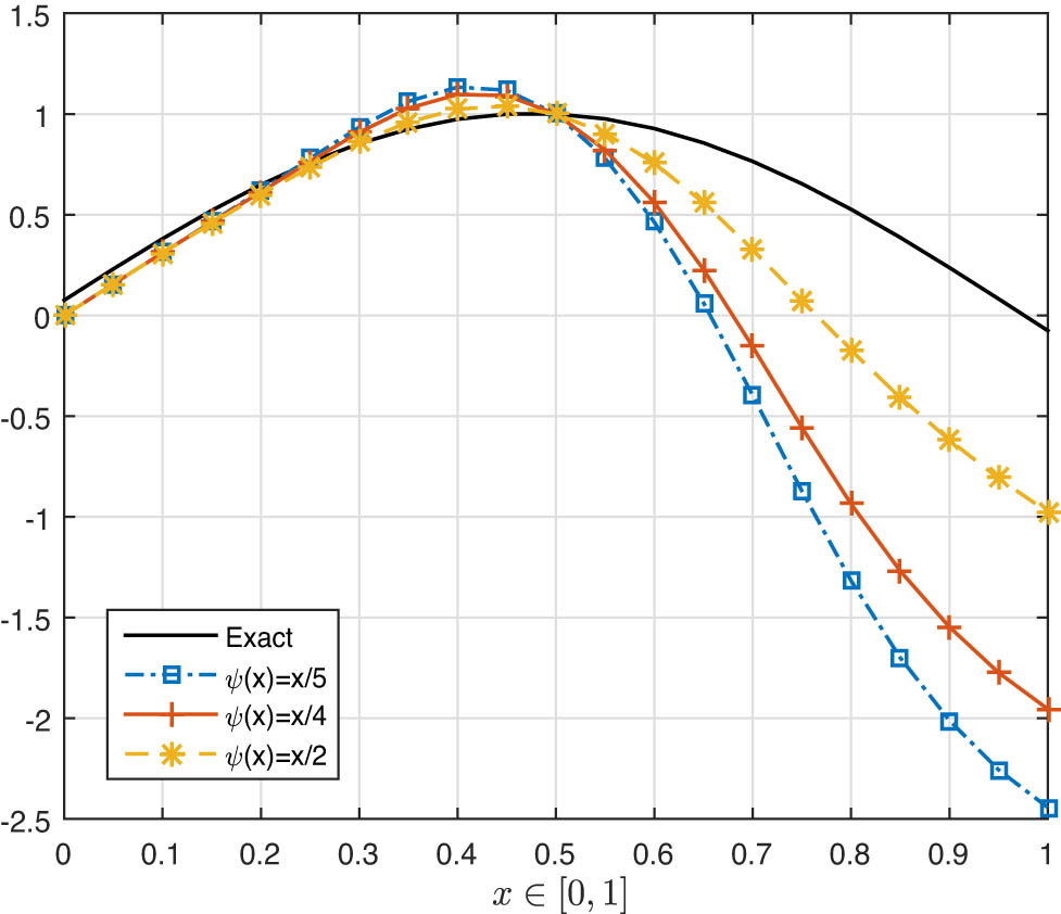
Example 4.3

Based on system (61), by taking ⅁ 1 ( x , u ) = cos ( π x ) 5 ( 1 + u 2 ) , ⅁ 2 ( x , u ) = cos ( π x ) 5 ( 3 + u ) , and

ℏ 1 ( u , ϶ 1 ( u ) ) = ( 1 + u 2 ) sin ( π u ϶ 1 3 ( u ) ) , ℏ 1 ( u , ϶ 2 ( u ) ) = ( 3 + u ) sin ( π u ϶ 2 3 ( u ) ) ,

we have the system of Volterra integral inclusions as follows:

(75) ϶ 1 ( x ) ∈ 0 , 1 5 ∫ 0 x cos ( π x ) sin ( π u ϶ 1 3 ( u ) ) d u + sin ( π x ) , ϶ 2 ( x ) ∈ 0 , 1 5 ∫ 0 x cos ( π x ) sin ( π u ϶ 2 3 ( u ) ) d u + sin ( π x ) ,

for x ∈ J , λ = 1 , where ζ = sin ( π x ) ∈ C ( J ) , multivalued ℏ 1 , ℏ 2 ∈ C ( J × R ) have non-empty compact values. The exact solution of the integral equation

(76) 1 5 ∫ 0 x cos ( π x ) sin ( π u ϶ 3 ( u ) ) d u + sin ( π x ) , x ∈ J ,

is ϶ ( x ) = sin ( π x ) + 1 3 ( 20 − 391 ) cos ( π x ) . Now, we can define two operators S , T : Y → Y as follows:

(77) T ϶ ( x ) = 1 5 ∫ 0 x cos ( π x ) sin ( π u ϶ 1 3 ( u ) ) d u + sin ( π x ) , S ϶ ( x ) = 1 5 ∫ 0 x cos ( π x ) sin ( π u ϶ 2 3 ( u ) ) d u + sin ( π x ) .

It follows that

(78) d s ( T ϶ 1 , S ϶ 2 ) = d s 1 5 ∫ 0 x cos ( π x ) sin ( π u ϶ 1 3 ( u ) ) d u + sin ( π x ) , 1 5 ∫ 0 x cos ( π x ) sin ( π u ϶ 2 3 ( u ) ) d u + sin ( π x ) = d s 1 5 ∫ 0 x cos ( π x ) sin ( π u ϶ 1 3 ( u ) ) d u , 1 5 ∫ 0 x cos ( π x ) sin ( π u ϶ 2 3 ( u ) ) d u ) = 1 5 d s ∫ 0 x cos ( π x ) sin ( π u ϶ 1 3 ( u ) ) d u , ∫ 0 x cos ( π x ) sin ( π u ϶ 2 3 ( u ) ) d u = 1 5 ∫ 0 x cos ( π x ) sin ( π u ϶ 1 3 ( u ) ) d u ⋅ ∫ 0 x cos ( π x ) sin ( π u ϶ 2 3 ( u ) ) d u ⩽ 1 5 ∫ 0 x cos ( π x ) d u 2 ∣ sin ( π u ϶ 1 3 ( u ) ) sin ( π u ϶ 2 3 ( u ) ) ∣ .

Thanks to Eq. (17), we obtain

M 2 ( ϶ 1 ( x ) , ϶ 2 ( x ) ) = max { d s ( ϶ 1 ( x ) , ϶ 2 ( x ) ) , d s ( ϶ 1 ( x ) , T ϶ 1 ( x ) ) , d s ( ϶ 2 ( x ) , S ϶ 2 ( x ) ) , d s ( ϶ 1 ( x ) , T ϶ 1 ( x ) ) + d s ( ϶ 1 ( x ) , S ϶ 2 ( x ) ) 2 , d s ( ϶ 1 ( x ) , T ϶ 2 ( x ) ) + d s ( ϶ 2 ( x ) , S ϶ 2 ( x ) ) 2 , d s ( ϶ 2 ( x ) , S ϶ 2 ( x ) ) 1 + d s ( ϶ 1 ( x ) , T ϶ 1 ( x ) ) 1 + d s ( ϶ 1 ( x ) , ϶ 2 ( x ) ) , d s ( ϶ 1 ( x ) , T ϶ 1 ( x ) ) 1 + d s ( ϶ 2 ( x ) , S ϶ 1 ( x ) ) 1 + d s ( ϶ 1 ( x ) , ϶ 2 ( x ) ) = max ϶ 1 ( x ) ϶ 2 ( x ) , ϶ 1 ( x ) 5 ∫ 0 x cos ( π x ) sin ( π u ϶ 1 3 ( u ) ) d u + ϶ 1 ( x ) sin ( π x ) , ϶ 2 ( x ) 5 ∫ 0 x cos ( π x ) sin ( π u ϶ 2 3 ( u ) ) d u + ϶ 2 ( x ) sin ( π x ) ,

(79) 1 2 ϶ 1 ( x ) 5 ∫ 0 x cos ( π x ) sin ( π u ϶ 1 3 ( u ) ) d u + ϶ 1 ( x ) sin ( π x ) + ϶ 1 ( x ) 5 ∫ 0 x cos ( π x ) sin ( π u ϶ 2 3 ( u ) ) d u + ϶ 1 ( x ) sin ( π x ) , 1 2 ϶ 1 ( x ) 5 ∫ 0 x cos ( π x ) sin ( π u ϶ 2 3 ( u ) ) d u + ϶ 1 ( x ) sin ( π x ) + ϶ 2 ( x ) 5 ∫ 0 x cos ( π x ) sin ( π u ϶ 2 3 ( u ) ) d u + ϶ 2 ( x ) sin ( π x ) , ϶ 2 ( x ) 5 ∫ 0 x cos ( π x ) sin ( π u ϶ 2 3 ( u ) ) d u + ϶ 2 ( x ) sin ( π x ) 1 + d s ( ϶ 1 ( x ) , T ϶ 1 ( x ) ) 1 + d s ( ϶ 1 ( x ) , ϶ 2 ( x ) ) , ϶ 1 ( x ) 5 ∫ 0 x cos ( π x ) sin ( π u ϶ 1 3 ( u ) ) d u + ϶ 1 ( x ) sin ( π x ) 1 + d s ( ϶ 2 ( x ) , S ϶ 1 ( x ) ) 1 + d s ( ϶ 1 ( x ) , ϶ 2 ( x ) ) ⩽ ϶ 1 ( x ) ⋅ ϶ 2 ( x ) .

Hence, by taking ψ ( x ) = x , we have

(80) ψ ( d s ( T ϶ 1 , S ϶ 2 ) ) ⩽ ψ ( M 2 ( ϶ 1 ( u ) , ϶ 2 ( u ) ) ) − φ ( M 2 ( ϶ 1 ( u ) , ϶ 2 ( u ) ) ) .

Table 1 displays the values of exact and suitable solutions of system (75) in Example 4.3 for ψ ( x ) = x 2 , x 4 , x 5 . Also, one can see the 2D plot of the results in Figure 1.

Therefore, system (75) has a solution based on common FPT for multi-valued operators.

Table 1

Results of exact and suitable solutions of system (75) in Example 4.3 for ψ ( x ) = x 2 , x 4 , x 5

x	Exact solution	ψ ( x ) = x 5		ψ ( x ) = x 4		ψ ( x ) = x 2
		Suitable solution	Error	Suitable solution	Error	Suitable solution	Error
0.00	0.0754	0.0000	0.0754	0.0000	0.0754	0.0000	0.0754
0.05	0.2309	0.1566	0.0744	0.1565	0.0744	0.1565	0.0744
0.10	0.3808	0.3110	0.0698	0.3106	0.0702	0.3098	0.0710
0.15	0.5212	0.4643	0.0569	0.4623	0.0589	0.4581	0.0631
0.20	0.6488	0.6201	0.0287	0.6137	0.0351	0.6007	0.0481
0.25	0.7604	0.7795	‒ 0.0191	0.7650	‒ 0.0046	0.7361	0.0244
0.30	0.8534	0.9344	‒ 0.0810	0.9093	‒ 0.0559	0.8592	‒ 0.0058
0.35	0.9253	1.0629	‒ 0.1377	1.0285	‒ 0.1033	0.9598	‒ 0.0345
0.40	0.9744	1.1336	‒ 0.1592	1.0971	‒ 0.1227	1.0241	‒ 0.0497
0.45	0.9995	1.1176	‒ 0.1181	1.0916	‒ 0.0921	1.0397	‒ 0.0402
0.50	1.0000	1.0000	0.0000	1.0000	0.0000	1.0000	0.0000
0.55	0.9759	0.7797	0.1962	0.8213	0.1546	0.9045	0.0714
0.60	0.9277	0.4630	0.4647	0.5606	0.3671	0.7558	0.1719
0.65	0.8568	0.0623	0.7944	0.2281	0.6287	0.5595	0.2972
0.70	0.7647	‒ 0.3968	1.1615	‒ 0.1556	0.9203	0.3267	0.4380
0.75	0.6538	‒ 0.8722	1.5260	‒ 0.5563	1.2101	0.0754	0.5784
0.80	0.5268	‒ 1.3171	1.8439	‒ 0.9361	1.4629	‒ 0.1742	0.7009
0.85	0.3868	‒ 1.6997	2.0865	‒ 1.2689	1.6557	‒ 0.4075	0.7943
0.90	0.2373	‒ 2.0107	2.2480	‒ 1.5468	1.7841	‒ 0.6189	0.8562
0.95	0.0819	‒ 2.2563	2.3382	‒ 1.7737	1.8557	‒ 0.8086	0.8906
1.00	‒ 0.0754	‒ 2.4428	2.3674	‒ 1.9542	1.8788	‒ 0.9771	0.9017

$Figure 1 Exact and suitable solution of system (75) in Example 4.3 when ψ ( x ) = x 2 , x 4 , x 5 \psi \left({\mathbb{x}})=\frac{{\mathbb{x}}}{2},\frac{{\mathbb{x}}}{4},\frac{{\mathbb{x}}}{5} .$

Figure 1

Exact and suitable solution of system (75) in Example 4.3 when ψ ( x ) = x 2 , x 4 , x 5 .

5 Conclusion

This article explores the generalization of the ( ψ , φ ) -type contraction in the context of super-metric space. The existence and uniqueness of specific rational-type contractions are ensured using the iteration technique and the characteristics of the super-metric spaces. Several corollaries have been deduced from the main results. Furthermore, the authenticity and reliability of the findings are achieved by an example. Moreover, the applications to an integral inclusion and fractal fractional partial differential equation are demonstrated. A numerical example and graph are also provided to strengthen the established existence results. These allow us to visually represent the solutions and demonstrate the behavior of the solutions. The presented results in this article improve our understanding of how mapping behaves in the context of super-metric space and highlight their use in the modeling and analysis of intricate dynamic systems.

mesamei@gmail.com

Acknowledgements

Muhammad Sarwar and Thabet Abdeljawad would like to thank Prince Sultan University for APC.

Funding information: The authors state no funding involved.
Author contributions: S. Khayyam Shah and M. Sarwar developed the concept of the original draft. Further they both performed theoretical formalism, and analytic calculations. M. Hleili and Mohammad Esmael Samei performed the numerical simulations and also reviewed and edited the final drafts. T. Abdelajwad completed the formal analysis and Visualization for the manuscript. M. Sarwar and T. Abdeljawad supervised the project. All authors read and approved the final manuscript.
Conflict of interest: The authors declare that they have no competing interests.
Data availability statement: Data sharing not applicable to this article as no datasets were generated or analyzed during the current study.

References

[1] Ali MU, Kamran T, Postolache M. Solution of Volterra integral inclusion in b-metric spaces via new fixed point theorem. Nonl Anal Model Control. 2017;22(1):17–30. 10.15388/NA.2017.1.2Search in Google Scholar

[2] Karapiiinar E, Abdeljawad T. Applying new fixed point theorems on fractional and ordinary differential equations. Adv Differ Equations. 2019;2019:421. 10.1186/s13662-019-2354-3Search in Google Scholar

[3] Dhage BC. A functional integral inclusion involving Carathéodories. Electron J Qualit Theory Differ Equ. 2003;14:1–18. 10.14232/ejqtde.2003.1.14Search in Google Scholar

[4] Singh R, Mishra J, Gupta VK. The dynamical analysis of a Tumor Growth model under the effect of fractal fractional Caputo-Fabrizio derivative. Int J Math Comput Eng. 2023;1:115–26. 10.2478/ijmce-2023-0009Search in Google Scholar

[5] O’Regan D. Integral inclusions of upper semi-continuous or lower semi-continuous type. Proceedings of the American Mathematical Society. 1996. p. 2391–9. 10.1090/S0002-9939-96-03456-9Search in Google Scholar

[6] Abodayeh K, Shah SK, Sarwar M, Promsakon C, Sitthiwirattham T. Ćirić-type generalized F-contractions with integral inclusion in super-metric spaces. Results Control Optimiz. 2024;16:100443. 10.1016/j.rico.2024.100443Search in Google Scholar

[7] Jan R, Boulaaras S, Alyobi S, Jawad M. Transmission dynamics of Hand-Foot-Mouth Disease with partial immunity through non-integer derivative. Int J Biomath. 2023;16(06):2250115. 10.1142/S1793524522501157Search in Google Scholar

[8] O’Regan D, Meehan M. Existence theory for nonlinear integral and integrodifferential equations. Netherlands: Springer; 2012. Search in Google Scholar

[9] Ata E, Kıymaz IO. New generalized Mellin transform and applications to partial and fractional differential equations. Int J Math Comput Eng. 2023;1(1):45–66. 10.2478/ijmce-2023-0004Search in Google Scholar

[10] Jan R, Boulaaras S, Alyobi S, Rajagopal K, Jawad M. Fractional dynamics of the transmission phenomena of dengue infection with vaccination. Discrete Contin Dyn Syst Ser S. 2022;16(8):2096–117. 10.3934/dcdss.2022154Search in Google Scholar

[11] Fatmawati F, Jan R, Khan MA, Khan Y, Ullah S. A new model of dengue fever in terms of fractional derivative. Math Biosci Eng. 2020;17(5):5267–88. 10.3934/mbe.2020285Search in Google Scholar PubMed

[12] Mlaiki N, Sagheer DeS, Noreen S, Batul S, Aloqaily A. Recent advances in proximity point theory applied to fractional differential equations. Axioms. 2024;13(6):395. 10.3390/axioms13060395Search in Google Scholar

[13] Erdogan F. A second order numerical method for singularly perturbed Volterra integro-differential equations with delay. Int J Math Comput Eng. 2024;2(1):85–96. 10.2478/ijmce-2024-0007Search in Google Scholar

[14] Jan A, Boulaaras S, Abdullah FA, Jan R. Dynamical analysis, infections in plants, and preventive policies utilizing the theory of fractional calculus. Europ Phys J Special Topics. 2023;232(14):2497–512. 10.1140/epjs/s11734-023-00926-1Search in Google Scholar

[15] Ali G, Khan RU, Kamran, Aloqaily A, Mlaiki N. On qualitative analysis of a fractional hybrid Langevin differential equation with novel boundary conditions. Boundary Value Problems. 2024;2024(1):62. 10.1186/s13661-024-01872-0Search in Google Scholar

[16] Jan R, Hinçal E, Hosseini K, Razak NNA, Abdeljawad T, Osman M. Fractional view analysis of the impact of vaccination on the dynamics of a viral infection. Alexandr Eng J. 2024;102:36–48. 10.1016/j.aej.2024.05.080Search in Google Scholar

[17] Abbas S, Ramzan M, Shafique A, Nazar M, Metwally ASM, Abduvalieva D, et al. Analysis of heat and mass transfer on nanofluid: An application of hybrid fractal-fractional derivative. Taylor & Francis: Numerical Heat Transfer, Part A: Applications. 2024. p. 1–14. 10.1080/10407782.2024.2366442Search in Google Scholar

[18] Kamran, SubhanA, Shah K, Subhi Aiadi S, Mlaiki N, Alotaibi FM. Analysis of Volterra integrodifferential equations with the fractal-fractional differential operator. Complexity. 2023;2023(1):7210126. 10.1155/2023/7210126Search in Google Scholar

[19] Karapinar E, Khojasteh F. Super metric spaces. Filomat. 2022;36(10):3545–9. 10.2298/FIL2210545KSearch in Google Scholar

[20] Karapinar E, Fulga A. Contraction in rational forms in the framework of super-metric spaces. Mathematics. 2022;10:3077. 10.3390/math10173077Search in Google Scholar

[21] Gourh R, Ughade M, Kumar Shukla M. On unique fixed-point theorems via interpolative and rational contractions in super-metric spaces. J Adv Math Comput Sci. 2024;39(2):11–9. 10.9734/jamcs/2024/v39i21865Search in Google Scholar

[22] Boyd DW, Wong JS. On nonlinear contractions. Proc Amer Math Soc. 1969;20:458–64. 10.2307/2035677Search in Google Scholar

[23] Alber YI, Guerre-Delabriere S. Principles of weakly contractive maps in Hilbert spaces. New Results Operat Theory Its Appl. 1997;98:7–22. 10.1007/978-3-0348-8910-0_2Search in Google Scholar

[24] Rhoades BE. Some theorems on weakly contractive maps. Nonl Anal Theory Methods Appl. 2001;47(4):2683–93. 10.1016/S0362-546X(01)00388-1Search in Google Scholar

[25] Dutta PN, Choudhary BS. A generalization of contraction principle in metric space. Fixed Point Theory Algorithms Sci Eng. 2008;2008:406368. 10.1155/2008/406368Search in Google Scholar

[26] Zhang Q, Song Y. Fixed point theory for generalized (ϕ)-weak contractions. Appl Math Lett. 2009;22(1):75–8. 10.1016/j.aml.2008.02.007Search in Google Scholar

[27] Dorić D. Common fixed point for generalized (ψ,ϕ)-weak contraction. Appl Math Lett. 2009;22(12):1896–900. 10.1016/j.aml.2009.08.001Search in Google Scholar

[28] He F, Sun YQ, Zhao XY. A common fixed point theorem for generalized (ψ,ϕ)-weak contractions of Suzuki type. J Math Anal. 2017;8(2):80–8. Search in Google Scholar

[29] Arya MC, Chandra N, Joshi MC. Fixed point of (ψ,ϕ)-contractions on metric spaces. J Anal. 2020;28(2):461–9. 10.1007/s41478-019-00181-5Search in Google Scholar

[30] Arya MC, Chandra N, Joshi MC. Common fixed point results for a generalized (ψ,ϕ)-rational contraction. Appl General Topol. 2023;24:129–44. 10.4995/agt.2023.18320Search in Google Scholar

Received: 2024-07-14

Revised: 2024-07-25

Accepted: 2024-08-12

Published Online: 2025-02-10

This work is licensed under the Creative Commons Attribution 4.0 International License.

Articles in the same Issue

https://doi.org/10.1515/nleng-2024-0032

Keywords for this article

positive solution; fixed point; fractional differential equation; Riemann-Liouville fractional derivative; existence and uniqueness

Creative Commons

BY 4.0