A modified fuzzy TOPSIS approach for the condition assessment of existing bridges
-
Bing Qu
 ,
Shiwei Lin
,
Shiwei Lin

Abstract
Bridge condition assessment is a crucial component of bridge management. To better adapt to the multi-level, nonlinear, and multi-criteria decision-making problems in bridge assessments, a modified technique for order preference by similarity to ideal solution (TOPSIS)-based nonlinear method is proposed in a fuzzy environment. First, quantitative representations of three different types of bottom indices of bridge assessment models under the analytic hierarchy process framework are developed using fuzzy numbers. Subsequently, with regard to the conventional TOPSIS approach, several enhancement and optimizations are considered, including the absolutization and fuzzification of positive and negative ideal solutions, the determination of variable weights of bottom-level indexes, fuzzy assessment based on level sets, and the defuzzification and grading of the evaluation results. These measures reduce the ambiguities and uncertainties associated with the conventional TOPSIS approach and can optimally accommodate bridge performance evaluation in fuzzy logic. Finally, to illustrate the practicality and feasibility of the developing method, a real bridge assessment scenario is built. The results indicate that this approach can effectively reflect the real state of the overall bridge, providing a robust basis for bridge maintenance and rehabilitation decision-making.
1 Introduction
In the past decades, due to the increase in the number of bridges being utilized, the health of bridge structures has gradually become a major concern for the society. Owing to design deficiencies, insufficient construction quality, overloading, combined environmental effects, and various complex and unforeseen service factors, which inevitably induce varying degrees of structural damage, a decrease in reliability, and even collapse, bridges deteriorate gradually [1,2]. Hence, it is essential to develop a systematic methodology for condition assessment, the result of which could be the decision-making basis for bridge maintenance, repair, and reinforcement.
In regard to the daily management of bridges, the most commonly utilized condition assessment method is based on evaluation standards or codes. Many countries have built the code systems for a customized bridge condition assessment, such as bridge inspector’s reference manual [3] and The manual for bridge evaluation (MBE) [4] in the USA; Standards for Technical Condition Evaluation of Highway Bridges [5] and Technical Standard of Maintenance for City Bridge [6] in China; and the Assessment of Highway Bridges and Structures (BD21/01) in the UK [7]. If we consider “Standards for Technical Condition Evaluation of Highway Bridges,” the technical condition grade of the bridge is determined by the weighted average score of each structural member with comprehensive considerations of the effect of bridge defects on safety, serviceability, and durability. The standard prescribes the divisions and weights of common members in detail; thus, by referencing it, executors are able to directly implement it, making the evaluation process quite simpler. Generally, standard-based approaches are convenient to implement, and with regard to daily inspection and assessment, they are applicable to most small and medium bridges. For more complicated bridges, however, the standard-based methods exhibit a lack of flexibility and objectivity, and they cannot reflect the complexity of the structures; thus, their applications are limited.
The analytic hierarchy process (AHP), a multi-criteria decision-making approach pioneered by Saaty in the 1970s [8], is one of the most commonly utilized comprehensive evaluation approaches for complicated bridges. AHP classifies the decision-making elements that could affect bridge performance into several hierarchies. Each hierarchy contains multiple indices, and a dominant or inclusive relationship exists between the upper and lower indices; thus, a disjoint orderly hierarchy network is formed. Subsequently, the relative importance of each index under their upper-layer index is determined using a similar pairwise comparison, and M (N i × N i ) (i = 1, 2…, M) judgment matrices are constructed, where M denotes the number of the total upper-layer indices and N i denotes the number of the lower-layer indices dominated by the ith upper-layer index. The absolute weight of each index can then be calculated by means of the M judgment matrices, which entails the utilization of an eigenvector approach or other methods. Subsequently, evaluated values of the bottom-layer indices are estimated; evaluations of the indices in other layers can be determined using some comprehensive evaluation method, and the overall evaluation result of the bridge is achieved [8]. Huang et al. established the condition assessment model for Harbin Songhua River Bridge (i.e., a long-span cable-stayed bridge) using uncertain AHP and optimal transfer matrix. The weights of assessment indices and the final assessment results of the bridge were calculated, showing the feasibility and practicability of this method [9]. Andrić and Lu considered various kinds of risk factors that may occur during the bridge service stage, analyzed the probability and possible consequences of the risks, and assessed the service risk with fuzzy AHP (FAHP); thus, they developed a convenient and reliable method for bridge safety management [10]. Shen et al. proposed a safety assessment method for concrete-filled steel tubular arch bridges AHP. It integrates component defect conditions and design load-bearing capacity as dual evaluation criteria, introduces an innovative exponential scale-based weighting approach for hierarchical analysis, and validates the system through finite element modeling and field inspections of the Jiantiao Bridge case study [11].
The efficiency of AHP is highly dependent on the accuracy and consistency of pairwise comparison judgment matrices; thus, numerous studies on scales of pairwise comparison, types of judgment matrices, and calculation of absolute weights have been performed [12,13,14]. Qu et al. utilized an exponential-interval scale to construct the judgment matrices, and they utilized the group decision theory on the basis of weighting set-valued statistics to calculate the absolute weight of each index; thus, they weakened the subjective uncertainty associated with conventional AHP assessment [15]. Xu et al. developed a five-grade exponential scale and utilized a genetic algorithm to optimize the consensus of judgment matrices. Subsequently, the particle swarm optimization-K-MEANS clustering algorithm was utilized to classify the experts’ opinions, and the weights were calculated using the peer-to-peer consensus reaching model. This method was applied to calculate the indicators’ weights in a suspension bridge evaluation model, and it exhibited more rational results than the codes [16].
Reliability analysis, which utilizes failure probability P f or reliability index β for the measurement of structural safety level, provides another perspective for bridge evaluation. It fully considers the uncertainty of loading and resistance by building reasonable probability evaluation models and by treating all factors as random variables. Wang et al. compared different assessment methods, which are described in AASHTO MBE in detail, and they proposed specific enhancements to current bridge-rating methods in a format that is consistent with the load and resistance factor rating option in AASHTO [17,18]. Gönen and Soyöz addressed the lack of standardized seismic assessment procedures for masonry arch bridges by proposing a reliability-based methodology integrating 3D finite element modeling, probabilistic nonlinear analysis, and performance limit states. It evaluates uncertainties in material properties and seismic inputs using Monte Carlo simulations and FORM, applied to a historical Turkish bridge to estimate failure probabilities and reliability indices for informed decision-making [19]. Furthermore, reliability analysis was utilized in bridge management system based on the results of inspections to give a life-cycle state assessment of bridges [20]. Frangopol et al. presented several approaches for incorporating monitoring data in structural reliability assessment based on performance prediction functions. Several numerical applications that utilize the monitoring data of several existing bridges were performed; thus, the adequacy and efficiency of the proposed approaches were demonstrated [21,22].
Technique for order preference by similarity to ideal solution (TOPSIS) is a method for multiple-criteria decision-making. It operates based on relative distances between alternatives and imposes no strict constraints on sample size [23]. TOPSIS requires only minimal computation, possesses clear geometric significance, and has found widespread application across various fields. Jena and Pradhan presented a novel combination comprising the artificial neural network cross-validation and analytic hierarchy process-technique for order of preference by similarity to ideal solution methods to enhance the earthquake risk assessment, and to test the model, they applied it to Aceh, Indonesia [24]. Mali et al. used the TOPSIS method to rank different bamboo species based on their physical and mechanical properties, selecting those suitable for use in building structures [25].
Bridge condition evaluation is a typical multi-criteria and nonlinear decision-making process that effectively coincides with TOPSIS. However, with respect to bridge condition assessment, TOPSIS-based research is still rare. Nurani et al. adopted the AHP, FAHP, and TOPSIS methods to conduct condition assessment and priority analysis on bridges in Kecamatan (District) Banjarsari, Surakarta. The three methods were compared, and the feasibility pertaining to the application of TOPSIS in bridge condition evaluation was demonstrated [26]. Li et al. proposed a fire vulnerability assessment framework for bridges by integrating susceptibility, resistance, and exposure factors utilizing a weighted TOPSIS method. It establishes graded indicators through qualitative–quantitative conversion, validates model feasibility via case analysis, and demonstrates alignment between evaluation results and historical fire performance [27]. Das Khan et al. developed an integrated AHP-fuzzy TOPSIS framework to prioritize concrete bridge defects by evaluating their root causes, addressing the oversight of causal factors in conventional assessments. A case study on an Indian bridge deck identifies cracks as the most critical defect, validated through sensitivity analysis, offering a systematic approach for infrastructure maintenance decisions [28].
Therefore, this study utilizes TOPSIS to perform the integrity-state assessment of bridges. To effectively adapt to the subjectivity and nonlinearity pertaining to bridge condition assessment, which enhances the reliability of evaluation, some enhancements are effected, including (a) fuzzy representation of the evaluated values of bottom-level indicators, (b) absolutization and fuzzification of positive and negative ideal solutions, (c) investigation of weight variation when evaluated values of indexes change, and (d) fuzzy assessment based on level sets and defuzzification. The preceding approach is applied to an existing arch bridge in Kunshan City, China, verifying its effectiveness.
2 Fuzzy representation of evaluated value for bottom-level indicators
The bottom-level indicators in the bridge condition assessment model are derived from the following items: visual inspection, field testing, or long-term monitoring. Furthermore, the evaluated value of each indicator is determined by the inspection result of the corresponding item. According to different properties, the bottom-level indicators can be classified into the following two categories (Figure 1):
Linguistic indicator: The linguistic indicator refers to inspection items that can be expressed through only qualitative linguistic description (i.e., words or sentences in a natural or artificial language), with no numerical test results; such inspection items include visual inspections of apparent defects on concrete and steel structures.
Numerical indicator: This type of indicator refers to inspection items that utilize inspection or monitoring instruments with quantitative values, for instance, crack width, concrete strength, and stress monitoring data. Based on different dimensions of measured results, the numerical indicator could be further subdivided into three subgroups: single-value indicators, space-series indicators, and time-series indicators. The evaluation of time-series indicators is mainly dependent on the immense structural health monitoring system data, which can be explored as a separate topic. Therefore, no in-depth discussion is offered herein.
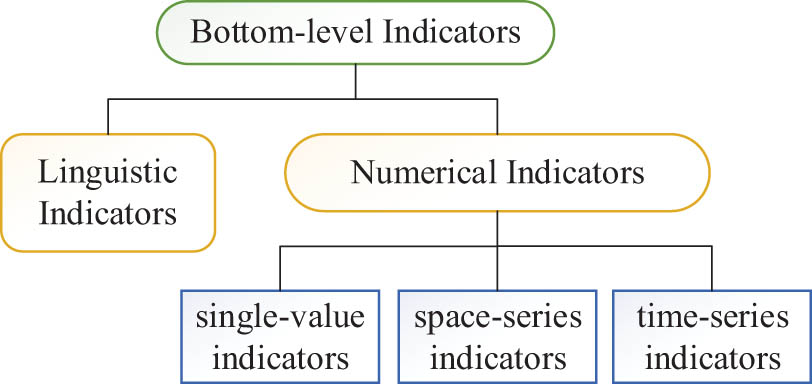
Classification of bottom-level indicators.
Different types of indicators exhibit different assessment methods and expressive forms. Therefore, it is necessary to build a suitable and uniform evaluation criterion for each type of indicator; thus, the evaluation results become dimensionlessly standardized and comparable to each other. With regard to the fuzziness and uncertainty in the appraisal process, a fuzzy grading system is presented; thus, all the information is represented in a more rational and concordant form.
2.1 Fuzzy representation of the evaluated values
A trapezoidal fuzzy number (Definition 1) is adopted to quantitatively describe the evaluation results of the bottom-level indicators.

Trapezoidal fuzzy membership function.
Definition 1
A quaternion
where a 1 and a 4 denote the lower and upper bound of the fuzzy number Ã, respectively, which reflect the scale of the fuzzy degree of Ã. A higher value of a 4 − a 1 indicates a higher ambiguity. [a 2, a 3] is the modal value range that corresponds to the most plausible probability. When a 2 = a 3, Ã is simplified to a triangular fuzzy number.
The justification for adopting a trapezoidal fuzzy grading system is rooted in its ability to effectively capture the multi-level uncertainties and subjective ambiguities inherent in bridge condition assessments. Unlike triangular fuzzy numbers, which assume a single peak value, trapezoidal fuzzy numbers provide a broader “plateau” interval [a 2, a 3] to represent the most plausible range of evaluated values, thereby accommodating the gradual transitions between adjacent linguistic terms (e.g., “poor” to “medium”). This feature aligns with the nonlinear and overlapping nature of defect severity gradations observed in real-world inspections (e.g., corrosion extent or crack width).
To quantify and unify the evaluation results, the standard centesimal system, in which the range of the fuzzy number is set at 0–100, is adopted, namely, a 1, a 2, a 3, a 4 ∈ [0, 100]. The fuzzy representation methods pertaining to the evaluated values of different types of indicators are introduced in the following contents.
2.2 Determination of evaluated values of linguistic indicators
To account for linguistic indicators (e.g., apparent inspection items), first, it is necessary to build appropriate linguistic terms that refer to the qualitative explanation of the rating levels, and determine their corresponding scores, herein, are performed as trapezoidal fuzzy numbers. These variables can be described by fuzzy numbers (Table 1) or by membership functions (Figure 3).
Linguistic terms for linguistic indicators
| Linguistic variables | Fuzzy evaluated value |
|---|---|
| Extremely poor (EP) | (0, 12, 18, 30) |
| Very poor (VP) | (15, 27, 33, 45) |
| Poor (P) | (30, 42, 48, 60) |
| Medium (M) | (45, 57, 63, 75) |
| Good (G) | (60, 72, 78, 90) |
| Very good (VG) | (75, 87, 93, 100) |
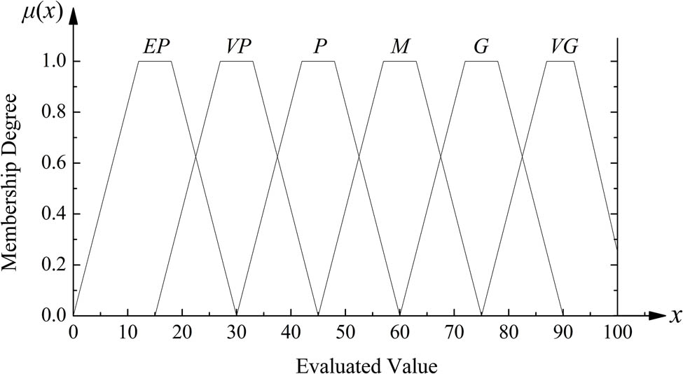
Membership function for linguistic indicators.
Herein, six linguistic terms are considered based on the evaluation results; thus, six different assessment rankings are represented. For different inspection items, it is necessary to assign particular linguistic attributes to each linguistic variable with reference to bridge inspection codes and the actual scenarios. If we consider “steel surface defect inspection,” the corresponding descriptions for the six linguistic terms are illustrated in Table 2. In the actual test, if the real scenario does not agree with any of the six grades, an intergraded trapezoidal fuzzy evaluated value can be utilized. Let
Linguistic terms for “steel surface defect inspection”
| No. | Linguistic variables | Descriptions | Fuzzy evaluated value |
|---|---|---|---|
| 1 | Extremely poor (EP) | The loss of metallic area exceeds 30%, with evident fracture and destruction | (0, 12, 18, 30) |
| 2 | Very poor (VP) | (a) The steel is immensely degenerated and deteriorated. The steelwork surface is immensely rusted (area: >60%). The loss of metallic area ranges from 15 to 30%. More than six holes, which are occasioned by corrosion, appear | (15, 27, 33, 45) |
| (b) The protective coating is almost worn out | |||
| (c) A lot of cracks appear on the surface | |||
| (d) Severe distortion is observed | |||
| 3 | Poor (P) | (a) The steel surface is severely rusted (area: 30–60%). The metallic area loss is 5–15%. Three to six holes, which are occasioned by corrosion, appear | (30, 42, 48, 60) |
| (b) Apparent aging and discoloration occur on the protective coating along with severe bubbling and peeling, and >60% of the total area is affected | |||
| (c) A certain number of crakes exist on the structural surface | |||
| (d) Abnormal deformation appears in individual members, and apparent vibration and shaking, accompanied by an abnormal sound, occur when driving | |||
| 4 | Medium (M) | (a) The steel surface is partly rusted (area: 15–30%). The metallic area loss is within 5%. A maximum of three holes, which are occasioned by corrosion, appear | (45, 57, 63, 75) |
| (b) Aging and discoloration occur on the protective coating along with partial bubbling and peeling, and 30–60% of the total area is affected | |||
| (c) A few crakes exist on the structural surface of the non-weld position | |||
| 5 | Good (G) | (a) The steel surface is partly rusted (affected area: 5–15%). The metallic area loss is within 2%, and only one hole, which is occasioned by corrosion, appears | (60, 72, 78, 90) |
| (b) Aging and discoloration occur on the protective coating along with partial bubbling and peeling, and <30% of the total area is affected | |||
| 6 | Very good (VG) | (a) The steel surface is basically intact without apparent damage, or it is somewhat rusty (affected area: <5%) | (75, 87, 93, 100) |
| (b) The protective coating is intact, or it exhibits low-level aging; the area that exhibits discoloration, bubbling, and peeling is <10% |
2.3 Determination of evaluated values pertaining to single-value indicators
Single-value indicators are those that possess only one certain numerical inspection result, such as crack width and carbonation depth in concrete.
Similar to the evaluation method of linguistic indicators, the grading tables of numerical judging criteria with corresponding evaluated ranges for single-value indicators can be formulated with reference to relevant specifications. Thus, the maximum and minimum inspected values (set as v h and v l , respectively) in each grade and the corresponding critical evaluated values (set as x h and x l , respectively) can be obtained. Furthermore, based on the measured data, the actual evaluated value (set as x) can be calculated using linear interpolation (set as v).
In regard to the relationship between the inspected value and the non-dimensional evaluated value, single-value indicators can be categorized as either direct index, inverse index, or combined index. A direct index refers to a single-value indicator whose test values are directly proportional to its non-dimensional evaluated values, whereas the inverse index is one whose test values are inversely proportional to its non-dimensional evaluated values. The assessment functions of direct and inverse indexes are listed in Eqs. (3) and (4).
Direct index function:
Inverse index function:
The combined index combines the direct and inverse indexes. An extreme point is defined at a certain inspected value, and the assessment function differs on each side of the extreme point, either on the direct index function or on the inverse index function.
The evaluated value, which is calculated using Eqs. (3) and (4), is certain, and it can be transformed into a trapezoidal fuzzy number by Eq. (5):
If we consider the rebar corrosion potential, five grades of judging criteria for rebar corrosion potential are defined as per “Specification for Inspection and Evaluation of Load-bearing Capacity of Highway Bridges” [29], and each of the rankings exhibits a corresponding evaluated range (Table 3).
Judging criteria and evaluated values for rebar corrosion potential
| Ranking | Potential (mV) | Rebar conditions | Evaluated range |
|---|---|---|---|
| 1 | 0 to −200 | No corrosion activity exists, or the corrosion activity is quite low | 85–100 |
| 2 | −200 to −300 | Corrosion activity exists, whereas the corrosion state is uncertain. Pitting corrosion may occur | 70–85 |
| 3 | −300 to −400 | Corrosion activity is comparatively high, and the probability of corrosion exceeds 90% | 65–70 |
| 4 | −400 to −500 | Corrosion activity is high, and high-level corrosion probably exists | 50–65 |
| 5 | <−500 | Members crack due to corrosion | 0–50 |
If the actual rebar corrosion potential is measured at 276 mV, which belongs to the second ranking as per Table 3, with the corresponding evaluated range of 70–85, the evaluated value could be calculated by the direct index function depicted as Eq. (5), namely,
2.4 Determination of evaluated values of spatial series indicators
For spatial series indicators, more than one inspected value is required for the assessment. Each inspected value corresponds to a separate inspection point at different positions on the structure; thus, a spatial distribution sequence is formed. Common spatial series indicators include the hanger force of an arch bridge and the alignment of the main beam.
Define the inspected values of spatial series indicators under the theoretical design state or under the actual as-built state of the bridge as the benchmark series; subsequently, the evaluated values of the spatial series indicators can be derived by comparing the newly measured series with the benchmark series. The comparison process is divided into two parts: (1) offset from benchmark series (i.e., uniform variation) and (2) irregular vibration from benchmark series (i.e., non-uniform variation). The eventual evaluated value is the product pertaining to the multiplication of the uniformly varying evaluated value by the non-uniformly varying evaluated value.
2.4.1 Uniformly varying evaluated value
Uniformly varying evaluated values of spatial series indicators were obtained using the following steps:
2.4.1.1 Determine the evaluated value on a single inspection point
First, calculate the evaluated value x vi at each inspection point; for example, calculate the tensile force of a certain hanger or the deflection of a certain section on the main beam. Subsequently, set the evaluated value under the benchmark status to 100 (i.e., the optimal state). When the inspected value offsets from the benchmark status to a higher degree, the inspection score becomes lower. Furthermore, there is a non-linear relationship between the inspected value and the evaluated value. Therefore, to describe the relationship between the inspected value and the corresponding evaluated value, a nonlinear combined index function is adopted, and the benchmark value is deemed as the extreme point. The non-linear function model for the calculation of the evaluated value x vi at each inspection point is expressed as follows:
where v i denotes the inspected value of the ith inspection point; v 0i denotes the benchmark value of the ith inspection point; x vi denotes the evaluated value of the ith inspection point; B denotes the shape factor that reflects the concavity and convexity, as well as the curvature change of the function; and B < 0. When B = 0, the function degrades into a linear variation. B is set at −0.5. v imin and v imax denote the maximum and minimum inspected values, respectively, when the evaluated value drops to 0, and they are expressed as follows:
where c min and c max denote the lower and upper bounds of the change ratio at the evaluated value of zero.
Figure 4 depicts the illustration pertaining to the evaluation function model of spatial series indicators (Eq. (6) on a single inspection point item.

Evaluation function model of spatial series indicators on a single inspection point.
The parameters in the evaluation model vary as per the different types of bridges and assessment indicators.
2.4.1.2 Determine the weight of each inspection point
The importance of different inspection points can be equal or different for a certain spatial series indicator. For different types of spatial series indicators, the weight determination methods are diverse.
Tu [30] utilized the bending strain energy of the main girder to reflect the influence of the stayed cables on the structure; thus, the researcher derived the initial weight of each stayed cable (Eq. (9)):
where U i denotes the bending strain energy of the main girder when the ith cable force changes by one unit, and it is expressed as follows:
The initial weight of each inspection point should be further modified by the actual evaluated values of the inspection points, and the variable-weight theory, which is discussed in Section 2.3, is utilized.
2.4.1.3 Determine the overall fuzzy evaluated value
First, fuzzify the evaluated value of a single measured item as follows:
Subsequently, calculate the general uniformly varying evaluated value, which is expressed as follows:
where
2.4.2 Non-uniformly varying evaluated value
The non-uniform variation of spatial series indicators refers to the irregular vibration of the observed series around the benchmark series. It can be quantified by the correlation degree between the benchmark series and the observed series. Herein, the gray correlation degree is utilized; thus, the correlation among the series is measured [31].
With respect to the order preservation effect after non-dimensional disposal and the relativity perspective during calculation, we utilize slope correlation to characterize the non-uniformly varying coefficient ξ, namely,
where v 0(k) denotes the benchmark value of the kth inspection point, and v s (k) denotes the actual measured value of the kth inspection point.
Thus, the eventual fuzzy evaluated value is expressed as follows:
3 Enhanced TOPSIS assessment method
3.1 Basic TOPSIS algorithm
Create the normalized decision matrix.
Suppose there are m projects to be assessed {H i (i = 1, 2, …, m)}, the H i th project contains n evaluation indicators {g j (j = 1, 2, …, n)}, and the evaluated value of indicator g j under project H i is a ij . Thus, a decision matrix A = (a ij ) m×n is established. The normalized decision matrix B = (b ij ) m×n is obtained by normalizing the decision matrix, where
(17)Determine the positive and negative ideal solutions:
(18)(19)Calculate the Euclidean distances of each index to the positive ideal solution
(20)where
Calculate the relative closeness as the evaluated value of the project:
C i reflects the extent to which the assessment object deviates from the negative ideal solution and approaches the positive ideal solution. A bigger C i value represents a better-evaluated result.
In regard to the defects of the conventional TOPSIS method and the limited practical robustness that characterizes its application in bridge-state assessment, some enhancements are presented herein, aiming at developing a more objective and accurate description of the actual bridge operational conditions, and the following aspects are considered.
3.2 Absolutization and fuzzification of positive and negative ideal solutions
The conventional TOPSIS method utilizes relative maximum and minimum values pertaining to assessment objects as the positive and negative ideal solutions; thus, it can achieve single evaluation and ranking. However, bridge-state assessment is a long-term dynamic process. When using relative values, the positive and negative ideal solutions become altered at different assessment times, and consequently, the evaluation results of each assessment are not comparable to each other. Therefore, it is necessary to set a fixed measurement standard, namely, absolutizing the positive and negative ideal solutions.
Therefore, the absolutized positive ideal solution of a certain evaluation index is defined as the optimal evaluated value when the index is under non-destructive conditions. While the absolutized negative ideal solution is defined as the worst evaluated value when the bridge is completely destroyed. Thus, the fuzzy positive ideal solution can be expressed as Eq. (22), with fuzzy medium â = 100:
Similarly, if we consider fuzzy medium â = 0, we could derive the fuzzy negative ideal solution as
3.3 Determination of variable weights of bottom-level indexes
In a k-level bridge condition assessment model (AHP model), let the weight of the rth index of the ith level
The relative weight of each index in different levels can be calculated as per the judgment matrix established by the AHP theory [15].
In regard to the nonlinear equilibrium of the assessment, the variable-weight concept is introduced. Let the fuzzy evaluated value of the bottom-level indicator g
r
be expressed as
Definition 2
Let
The existence of a balance function
Thus, the variable weight can be obtained via the construction of an appropriate state variable-weight vector or balance function.
The variable weight of each index in the bridge condition assessment should meet the following axiomatic requirements:
Normality:
Continuity:
Penalization:
The properties and construction of the state variable-weight vector and balance function have been analyzed in many studies [32,33,34]. Herein, relevant studies are referenced, and an exponential-state variable-weight vector is established as follows:
where α denotes the balance factor, reflecting the tolerance level of decision-makers to the defects of evaluation indicators, and
Upon substituting Eq. (27) into Eq. (25), we obtain the following expression:
Definition 3
Let
where
The weight-adjustment level K reflects the adjustment effect and equilibrium of
Thus, for the state variable-weight vector presented in Eq. (27), we obtain the following expression:
Consequently,
It is observed that the weight-adjustment level K of
3.4 Fuzzy assessment based on level sets and defuzzification of the evaluation results
Definition 4
Given a fuzzy set
The λ-level set of
The level set is a crucial component of the mutual transformation between fuzzy sets and ordinary sets. Let the bottom-level index set be {g
j
(j = 1, 2, …, n)}, and let the fuzzy evaluated value of index g
r
be
Furthermore, the λ-level set of
The positive and negative ideal solution intervals corresponding to the λ-level set, which are obtained by the fuzzy positive and negative ideal solutions determined by Eqs. (22) and (23), are expressed as follows:
Following the variable weight of each bottom-level indicator determined by Eq. (25), and combined with Eqs. (20) and (21), the relative closeness between the bridge’s actual operational and ideal state under a certain λ-level is rewritten as follows:
Apparently, C
λ
is an interval number under every λ-level set. Because it can easily be demonstrated that
where
Thus, the final relative closeness
Generally, N = 11, namely,
PC denotes the final evaluated bridge condition assessment value.
3.5 Grading of evaluation results
The bridge condition assessment evaluation result that utilizes the enhanced TOPSIS method (PC value) is relative closeness, which ranges from 0 to 1. When the result is closer to 1, the bridge is in a more optimal condition. Bridge health condition is divided into five grades as per the PC value interval (Table 4).
TOPSIS grading bridge evaluation standard
| Grade | PC value | Status | Countermeasures |
|---|---|---|---|
| A level | 0.90–1 | Good | Daily maintenance |
| B level | 0.75–0.90 | Normal | Daily maintenance; small repairs after special inspections |
| C level | 0.60–0.75 | Middle | Medium repairs after comprehensive inspections |
| D level | 0.45–0.60 | Weak | Heavy repairs or reinforcement |
| E level | 0–0.45 | Dangerous | Reinforcement with bridge close, reconstruction, and extension |
4 Case study
For the case study, Kunshan Yufeng Bridge, located in Kunshan City of China, which is a non-thrusting leaning-type arch bridge with an 110 m main span, is chosen (Figure 5). The condition assessment of the main bridge is performed using data obtained from one of the inspections. Table 5 depicts the assessment model indicators, combined weight, fuzzy evaluated value, and variable weight of each bottom-level indicator. There are several notable points. (1) The assessment model is alterable; decision-makers can further decompose, synthesize, or modify the indicators at all levels as per the actual demand. (2) The combined weights depicted in Table 5 are estimated by the method proposed by Qu et al. [15]. (3) The fuzzy evaluated values are determined by the method presented in Section 1 based on the on-site inspection data. (4) The variable weights are calculated using Eq. (30) with the weight-adjustment level set at K = 0.8.

Kunshan Yufeng Bridge.
Weights and fuzzy evaluated values of bottom-level indicators
| The first-level indicator (
|
The second-level indicator (
|
The bottom-level indicator (
|
Combined weight
|
Fuzzy evaluated value
|
Variable weight
|
|---|---|---|---|---|---|
| Main Arch rib (0.194) | — | Steel surface defect (0.266) | 0.05160 | (76, 88, 94, 100) | 0.03585 |
| — | Welds and joints (0.394) | 0.07644 | (70, 82, 88, 100) | 0.07620 | |
| — | Deformation (0.243) | 0.04714 | (77.2, 89.2, 95.2, 100) | 0.03047 | |
| — | Protective coating (0.097) | 0.01882 | (80, 92, 98, 100) | 0.01028 | |
| Inclined arch rib (0.115) | — | Steel surface defect (0.266) | 0.03059 | (74, 86, 92, 100) | 0.02397 |
| — | Welds and joints (0.394) | 0.04531 | (75, 87, 93, 100) | 0.03343 | |
| — | Deformation (0.243) | 0.02795 | (77.3, 89.3, 95.3, 100) | 0.01795 | |
| — | Protective coating (0.097) | 0.01116 | (75, 87, 93, 100) | 0.00823 | |
| Vertical and horizontal beam systems (0.207) | Main beam (0.252) | Steel surface defect (0.266) | 0.01388 | (74, 86, 92, 100) | 0.01087 |
| Welds and joints (0.394) | 0.02055 | (73, 85, 91, 100) | 0.01710 | ||
| Deformation (0.243) | 0.01268 | (78.1, 90.1, 96.1, 100) | 0.00776 | ||
| Protective coating (0.097) | 0.00506 | (76, 88, 94, 100) | 0.00352 | ||
| Small longitudinal beam (0.163) | Steel surface defect (0.266) | 0.00898 | (76.5, 88.5, 94.5, 100) | 0.00605 | |
| Welds and joints (0.394) | 0.01329 | (77, 89, 95, 100) | 0.00870 | ||
| Deformation (0.243) | 0.00820 | (77.1, 89.1, 95.1, 100) | 0.00533 | ||
| Protective coating (0.097) | 0.00327 | (73, 85, 91, 100) | 0.00272 | ||
| End cross-beam and stiffening arch (0.195) | Steel surface defect (0.266) | 0.01074 | (73, 85, 91, 100) | 0.00894 | |
| Welds and joints (0.394) | 0.01590 | (71, 83, 89, 100) | 0.01493 | ||
| Deformation (0.243) | 0.00981 | (78.6, 90.6, 96.6, 100) | 0.00583 | ||
| Protective coating (0.097) | 0.00392 | (74, 86, 92, 100) | 0.00307 | ||
| Normal cross-beam (0.145) | Steel surface defect (0.266) | 0.00798 | (76, 88, 94, 100) | 0.00555 | |
| Welds and joints (0.394) | 0.01183 | (76, 88, 94, 100) | 0.00822 | ||
| Deformation (0.243) | 0.00729 | (77.2, 89.2, 95.2, 100) | 0.00471 | ||
| Protective coating (0.097) | 0.00291 | (74, 86, 92, 100) | 0.00228 | ||
| Outrigger beam (0.117) | Steel surface defect (0.266) | 0.00644 | (77, 89, 95, 100) | 0.00421 | |
| Welds and joints (0.394) | 0.00954 | (75, 87, 93, 100) | 0.00704 | ||
| Deformation (0.243) | 0.00589 | (72.3, 84.3, 90.3, 100) | 0.00511 | ||
| Protective coating (0.097) | 0.00235 | (68, 80, 86, 98) | 0.00264 | ||
| Concrete deck slab (0.128) | Surface map cracking (0.203) | 0.00538 | (71, 83, 89, 100) | 0.00505 | |
| Concrete spalling (0.184) | 0.00488 | (79, 91, 97, 100) | 0.00283 | ||
| Rusting of exposed steel bars (0.326) | 0.00864 | (80, 92, 98, 100) | 0.00472 | ||
| Water seepage (0.287) | 0.00760 | (78, 90, 96, 100) | 0.00468 | ||
| Main hanger (0.152) | — | Hanger force (0.339) | 0.05153 | (74.1, 86.1, 92.1, 100) | 0.04013 |
| — | Hanger surface defect (0.267) | 0.04058 | (72, 84, 90, 100) | 0.03587 | |
| — | Anchor system (0.394) | 0.05989 | (48, 60, 66, 78) | 0.22448 | |
| Inclined hanger (0.101) | — | Hanger force (0.339) | 0.03424 | (75.4, 87.4, 93.4, 100) | 0.02466 |
| — | Hanger surface defect (0.267) | 0.02697 | (77, 89, 95, 100) | 0.01764 | |
| — | Anchor system (0.394) | 0.03979 | (75, 87, 93, 100) | 0.02936 | |
| Pier and foundation (0.162) | — | Uniform settlement (0.144) | 0.02333 | (78.8, 90.8, 96.8, 100) | 0.01369 |
| — | Differential settlement (0.356) | 0.05767 | (76.7, 88.7, 94.7, 100) | 0.03841 | |
| — | Concrete quality (0.273) | 0.04423 | (74, 86, 92, 100) | 0.03466 | |
| — | Foundation scour (0.227) | 0.03677 | (75, 87, 93, 100) | 0.02713 | |
| Ancillary facility (0.069) | Bridge deck pavement (0.293) | Crack (0.305) | 0.00617 | (76, 88, 94, 100) | 0.00428 |
| Loose and pothole (0.382) | 0.00772 | (81, 93, 99, 100) | 0.00397 | ||
| Slurry (0.187) | 0.00378 | (82, 94, 100, 100) | 0.00183 | ||
| Pavement roughness (0.126) | 0.00255 | (81, 93, 99, 100) | 0.00131 | ||
| Bearing (0.408) | Displacement (0.673) | 0.01895 | (75, 87, 93, 100) | 0.01398 | |
| Surface defect (0.327) | 0.00921 | (71, 83, 89, 100) | 0.00864 | ||
| — | Drainage system (0.070) | 0.00483 | (66, 78, 84, 96) | 0.00613 | |
| Sidewalk and rail (0.098) | Sidewalk (0.437) | 0.00295 | (68, 80, 86, 98) | 0.00332 | |
| Rail and fence (0.563) | 0.00381 | (71, 83, 89, 100) | 0.00357 | ||
| — | Expansion joint (0.131) | 0.00904 | (34, 46, 52, 64) | 0.07870 |
The interval-relative closenesses under the level sets
Fuzzy relative closeness at each λ-level cut set
| λ | Relative closeness | λ | Relative closeness |
|---|---|---|---|
| 0 | (0.7332, 0.8433) | 0.6 | (0.7524, 0.8100) |
| 0.1 | (0.7366, 0.8380) | 0.7 | (0.7553, 0.8044) |
| 0.2 | (0.7399, 0.8325) | 0.8 | (0.7581, 0.7987) |
| 0.3 | (0.7431, 0.8269) | 0.9 | (0.7609, 0.7932) |
| 0.4 | (0.7463, 0.8213) | 1.0 | (0.7637, 0.7876) |
| 0.5 | (0.7494, 0.8157) |
The final evaluated PC value is obtained by defuzzifying the aforementioned fuzzy outputs, and it is calculated as follows:
The PC value indicates a Grade B bridge status, in which small repairs are required after special inspections. The relatively lower comprehensively evaluated value of the bridge is mainly occasioned by the poor performance of two indicators, namely, “Main hanger-Anchor system” and “Ancillary facility–Expansion joint,” with the fuzzy evaluated values set at (48, 60, 66, 78) and (34, 46, 52, 64), respectively. For the anchor systems of the main hangers, a large number of rust stains were observed on the surface pertaining to the upper anchor cup of one short hanger rod, and the rust stains were probably occasioned by the outflow of the rust water contained in the anchor cup (Figure 6(a)). Therefore, it is essential to further ascertain the source of the rust water, the rusting areas, and the degree of corrosion, and conduct special maintenance. On the other hand, the two bridge expansion joints were severely aged and damaged accompanied by a serious disintegration, and replacement was necessary (Figure 6(b)). Due to the variable-weight effect, the weight of the index “Main hanger–Anchor system” increased from 0.05989 to 0.22484, and the weight of “Ancillary facility–Expansion joint” increased from 0.00904 to 0.07870.

Inspection disease: (a) anchor system of the main hanger and (b) expansion joint.
Suppose that the evaluated “Main hanger–Anchor system” and “Ancillary facility–Expansion joint” values were set at (75, 87, 93, 100) and (81, 93, 99, 100), respectively; after the repair, the new PC value could be recalculated as
PC new = 0.9196.
The bridge condition level is upgraded to Grade A, which exhibits a “good” status and requires only daily maintenance.
To explore the similarity and difference between the conventional TOPSIS method and the enhanced one, the fuzzy evaluated values of “Main hanger–Anchor system” and “Ancillary facility–expansion joint” are treated as variable inputs with the medium varying from 0 to 100; by contrast, the evaluated values of other indicators remain unaltered (Table 5). Calculate the comprehensively evaluated values of the bridge using these two methods. When employing the conventional TOPSIS method, the absolute values (i.e., 100 and 0) are still utilized as the positive and negative ideal solutions, and the evaluated values of the bottom-level indexes are represented by the medium of the corresponding fuzzy evaluated values.
The curve of the integrity assessment results (PC values) obtained from the two methods is depicted in Figure 7.

Comparison of the integrity assessment results pertaining to the conventional and enhanced TOPSIS methods: (a) “Main hanger–Anchor system” and (b) “Ancillary facility–Expansion joint” as variables.
Figure 7 indicates that the difference between the two methods is more significant for the index with a larger combined weight, namely, the “Main hanger–Anchor system” index. For a single indicator, when the evaluated value is lower, the distinction between the two methods is greater. For instance, when the evaluated medium value of the “Main hanger–Anchor system” is 20, the PC value under conventional TOPSIS is 0.7947, whereas that under enhanced TOPSIS is only 0.3682; therefore, it is apparent that an immensely crucial disease, which may even affect the overall safety of the bridge, has occurred in the anchor system. However, the bridge is allocated a Level B grade, which indicates that in the conventional TOPSIS method, it is still in a “normal” status, which is apparently not consistent with the actual scenario.
5 Discussion
The bottom-level indicators of bridge structures are divided into linguistic indicators, single-value indicators, and spatial series indicators. A fuzzy assessment system of the bottom-level indicators is established; thus, the subjectivity and uncertainty in the evaluation process are weakened.
The variable-weight concept is introduced. The exponential state variable-weight vector is constructed, and the reasonable weight-adjustment level is discussed; thus, the weights of the indicators increase exponentially as their evaluated values decrease. Therefore, indicators exhibiting lower combined weights can be reflected in the overall state assessment with greater importance when their evaluated values are being reduced; thus, decision-making errors are effectively prevented.
The calculation of the fuzzy interval relative closeness and the defuzzification of the evaluation results are investigated using the level set theory. Moreover, the grading standard and decision-making categories of bridge evaluation are developed; thus, the method can adapt to the thinking habits of decision-makers, and to management and maintenance needs.
Herein, an integrity assessment of Kunshan Yufeng Bridge is implemented using on-site inspection data; the enhanced TOPSIS method is adopted, and the method is compared with the conventional TOPSIS method. The results indicate that compared with the conventional TOPSIS method, the enhanced TOPSIS method can effectively address the actual bridge condition assessment needs and that it exhibits optimal scientificity and accuracy; thus, an effective method for bridge health assessment is developed.
Acknowledgments
This work was supported by the “Natural Science Foundation of Fujian Province” under Grant [Numbers 2023J01998, 2023J01999, 2024J01876], the “Science and Technology Project of Putian City” under Grant [Number 2022GZ2001ptxy13], and the “Startup Fund for Advanced Talents of Putian University” under Grant [Number 2023136].
-
Funding information: The authors state no funding involved.
-
Author contributions: Bing Qu wrote the main manuscript text and was responsible for the overall design, refinement, and validation of the method. Shiwei Lin and Haisheng Huang contributed to the construction and evaluation of the hierarchical model. All authors have accepted responsibility for the entire content of this manuscript and approved its submission.
-
Conflict of interest: The authors state no conflict of interest.
-
Data availability statement: All data generated or analyzed during this study are included in this published article.
References
[1] Hao H, Bi K, Chen W, Pham TM, Li J. Towards next generation design of sustainable, durable, multi-hazard resistant, resilient, and smart civil engineering structures. Eng Struct. 2023;277:115477.10.1016/j.engstruct.2022.115477Suche in Google Scholar
[2] Leoni L, BahooToroody A, Abaei MM, Cantini A, BahooToroody F, De Carlo F. Machine learning and deep learning for safety applications: Investigating the intellectual structure and the temporal evolution. Saf Sci. 2024;170:106363.10.1016/j.ssci.2023.106363Suche in Google Scholar
[3] Ryan TW, Lloyd CE, Pichura MS, Tarasovich DM, Fitzgerald S. Bridge inspector’s reference manual (BIRM). Arlington: National Highway Institute (US); 2022.Suche in Google Scholar
[4] Transportation Officials. Subcommittee on Bridges. The manual for bridge evaluation. Washington, D.C.: American Association of State Highway and Transportation Officials; 2011.Suche in Google Scholar
[5] MOT (Ministry of Transport of the People’s Republic of China). Standards for technical condition evaluation of highway bridges. Beijing: China Communications Press; 2011.Suche in Google Scholar
[6] Ministry of Housing and Urban-Rural Development of the People’s Republic of China. Technical Standard of Maintenance for City Bridge. Beijing: China Architecture & Building Press; 2017.Suche in Google Scholar
[7] HA (Highways Agency). The assessment of highway bridges and structures. London: The Stationery Office (UK); 2001.Suche in Google Scholar
[8] Saaty TL. The analytic hierarchy process (AHP). J Oper Res Soc. 1980;41(11):1073–6.10.1038/sj/jors/0411110Suche in Google Scholar
[9] Huang Q, Ren Y, Lin YZ. Uncertain type of AHP method in comprehensive assessment of long span bridge. J Highw Transp Res Dev. 2008;3(144):79–83.Suche in Google Scholar
[10] Andrić JM, Lu DG. Risk assessment of bridges under multiple hazards in operation period. Saf Sci. 2016;83:80–92.10.1016/j.ssci.2015.11.001Suche in Google Scholar
[11] Shen P, Chen Y, Ma S, Yan Y. Safety assessment method of concrete-filled steel tubular arch bridge by fuzzy analytic hierarchy process. Buildings-Basel. 2023;14(1):67.10.3390/buildings14010067Suche in Google Scholar
[12] Dutta B, Labella Á, Ishizaka A, Martínez L. Eliciting personalized AHP scale from verbal pairwise comparisons. J Oper Res Soc. 2025;76(3):541–53.10.1080/01605682.2024.2376033Suche in Google Scholar
[13] Cavallo B, Ishizaka A. Evaluating scales for pairwise comparisons. Ann Oper Res. 2023;325(2):951–65.10.1007/s10479-022-04682-8Suche in Google Scholar
[14] Pant S, Kumar A, Ram M, Klochkov Y, Sharma HK. Consistency indices in analytic hierarchy process: a review. Mathematics-Basel. 2022;10(8):1206.10.3390/math10081206Suche in Google Scholar
[15] Qu B, Xiao RC, Zhong J, Lin J. Application of improved AHP and group decision theory in bridge assessment. J Cent South Univ (Sci Technol). 2015;46:4204–10.Suche in Google Scholar
[16] Xu X, Huang Q, Ren Y, Liu X. Determination of index weights in suspension bridge condition assessment based on group-AHP. J Hunan Univ (Nat Sci). 2018;45(3):122–8.Suche in Google Scholar
[17] Wang N, O’Malley C, Ellingwood BR, Zureick AH. Bridge rating using system reliability assessment. I: Assessment and verification by load testing. J Bridge Eng. 2011;16(6):854–62.10.1061/(ASCE)BE.1943-5592.0000172Suche in Google Scholar
[18] Wang N, Ellingwood BR, Zureick AH. Bridge rating using system reliability assessment. II: Improvements to bridge rating practices. J Bridge Eng. 2011;16(6):863–71.10.1061/(ASCE)BE.1943-5592.0000171Suche in Google Scholar
[19] Gönen S, Soyöz S. Reliability-based seismic performance of masonry arch bridges. Struct Infrastruct E. 2022;18(12):1658–73.10.1080/15732479.2021.1918726Suche in Google Scholar
[20] Frangopol DM, Kim S. Bridge safety, maintenance and management in a life-cycle context. Boca Raton: CRC Press; 2022.10.1201/9781003196877Suche in Google Scholar
[21] Frangopol DM, Strauss A, Kim S. Bridge reliability assessment based on monitoring. J Bridge Eng. 2008;13(3):258–70.10.1061/(ASCE)1084-0702(2008)13:3(258)Suche in Google Scholar
[22] Frangopol DM, Strauss A, Kim S. Use of monitoring extreme data for the performance prediction of structures: General approach. Eng Struct. 2008;30(12):3644–53.10.1016/j.engstruct.2008.06.010Suche in Google Scholar
[23] Yoon KP, Hwang CL. Multiple attribute decision making: an introduction. Thousand Oaks: Sage Publications; 1995.10.4135/9781412985161Suche in Google Scholar
[24] Jena R, Pradhan B. Integrated ANN-cross-validation and AHP-TOPSIS model to improve earthquake risk assessment. Int J Disast Risk Re. 2020;50:101723.10.1016/j.ijdrr.2020.101723Suche in Google Scholar
[25] Mali PR, Vishwakarma RJ, Isleem HF, Khichad JS, Patil RB. Performance evaluation of bamboo species for structural applications using TOPSIS and VIKOR: A comparative study. Constr Build Mater. 2024;449:138307.10.1016/j.conbuildmat.2024.138307Suche in Google Scholar
[26] Nurani AI, Pramudyaningrum AT, Fadhila SR, Sangadji S, Hartono W. Analytical hierarchy process (AHP), fuzzy AHP, and TOPSIS for determining bridge maintenance priority scale in Banjarsari, Surakarta. Int J Sci Appl Sci Conf. 2017;2(1):60.10.20961/ijsascs.v2i1.16680Suche in Google Scholar
[27] Li Q, Guo H, Zhou J, Wang M. Bridge fire vulnerability hierarchy assessment based on the weighted topsis method. Sustainability-Basel. 2022;14(21):14174.10.3390/su142114174Suche in Google Scholar
[28] Das Khan S, Datta AK, Topdar P, Sagi SR. A cause-based defect ranking approach for existing concrete bridges using Analytic Hierarchy Process and fuzzy-TOPSIS. Struct Infrastruct E. 2023;19(11):1555–67.10.1080/15732479.2022.2035407Suche in Google Scholar
[29] MOT (Ministry of Transport of the People’s Republic of China). Specification for Inspection and Evaluation of Load-bearing Capacity of Highway Bridges. Beijing: China Communications Press; 2011.Suche in Google Scholar
[30] Tu X. Research on technical Condition evaluation of long Span Cable-stayed Bridge based on detection [dissertation]. Shanghai: Tongji University; 2009.Suche in Google Scholar
[31] Lan H, Shi JJ. Degree of grey incidence and variable weight synthesizing applied in bridge assessment. J Tongji Univ Nat Sci. 2001;29(1):50–4.Suche in Google Scholar
[32] Li DQ, Li HX. Analysis of variable weights effect and selection of appropriate state variable weights vector in decision making. Control Decis. 2004;19(11):1241–5.Suche in Google Scholar
[33] Li D, Hao F. Weights transferring effect of state variable weight vector. Syst Eng Theor Pract. 2009;29(6):127–31.10.1016/S1874-8651(10)60054-3Suche in Google Scholar
[34] Li D, Zeng W. The effectiveness of balance function in variable weights decision making. Syst Eng Theor Pract. 2016;36(3):712–8.Suche in Google Scholar
© 2025 the author(s), published by De Gruyter
This work is licensed under the Creative Commons Attribution 4.0 International License.
Artikel in diesem Heft
- Research Articles
- Generalized (ψ,φ)-contraction to investigate Volterra integral inclusions and fractal fractional PDEs in super-metric space with numerical experiments
- Solitons in ultrasound imaging: Exploring applications and enhancements via the Westervelt equation
- Stochastic improved Simpson for solving nonlinear fractional-order systems using product integration rules
- Exploring dynamical features like bifurcation assessment, sensitivity visualization, and solitary wave solutions of the integrable Akbota equation
- Research on surface defect detection method and optimization of paper-plastic composite bag based on improved combined segmentation algorithm
- Impact the sulphur content in Iraqi crude oil on the mechanical properties and corrosion behaviour of carbon steel in various types of API 5L pipelines and ASTM 106 grade B
- Unravelling quiescent optical solitons: An exploration of the complex Ginzburg–Landau equation with nonlinear chromatic dispersion and self-phase modulation
- Perturbation-iteration approach for fractional-order logistic differential equations
- Variational formulations for the Euler and Navier–Stokes systems in fluid mechanics and related models
- Rotor response to unbalanced load and system performance considering variable bearing profile
- DeepFowl: Disease prediction from chicken excreta images using deep learning
- Channel flow of Ellis fluid due to cilia motion
- A case study of fractional-order varicella virus model to nonlinear dynamics strategy for control and prevalence
- Multi-point estimation weldment recognition and estimation of pose with data-driven robotics design
- Analysis of Hall current and nonuniform heating effects on magneto-convection between vertically aligned plates under the influence of electric and magnetic fields
- A comparative study on residual power series method and differential transform method through the time-fractional telegraph equation
- Insights from the nonlinear Schrödinger–Hirota equation with chromatic dispersion: Dynamics in fiber–optic communication
- Mathematical analysis of Jeffrey ferrofluid on stretching surface with the Darcy–Forchheimer model
- Exploring the interaction between lump, stripe and double-stripe, and periodic wave solutions of the Konopelchenko–Dubrovsky–Kaup–Kupershmidt system
- Computational investigation of tuberculosis and HIV/AIDS co-infection in fuzzy environment
- Signature verification by geometry and image processing
- Theoretical and numerical approach for quantifying sensitivity to system parameters of nonlinear systems
- Chaotic behaviors, stability, and solitary wave propagations of M-fractional LWE equation in magneto-electro-elastic circular rod
- Dynamic analysis and optimization of syphilis spread: Simulations, integrating treatment and public health interventions
- Visco-thermoelastic rectangular plate under uniform loading: A study of deflection
- Threshold dynamics and optimal control of an epidemiological smoking model
- Numerical computational model for an unsteady hybrid nanofluid flow in a porous medium past an MHD rotating sheet
- Regression prediction model of fabric brightness based on light and shadow reconstruction of layered images
- Dynamics and prevention of gemini virus infection in red chili crops studied with generalized fractional operator: Analysis and modeling
- Qualitative analysis on existence and stability of nonlinear fractional dynamic equations on time scales
- Fractional-order super-twisting sliding mode active disturbance rejection control for electro-hydraulic position servo systems
- Analytical exploration and parametric insights into optical solitons in magneto-optic waveguides: Advances in nonlinear dynamics for applied sciences
- Bifurcation dynamics and optical soliton structures in the nonlinear Schrödinger–Bopp–Podolsky system
- User profiling in university libraries by combining multi-perspective clustering algorithm and reader behavior analysis
- Exploring bifurcation and chaos control in a discrete-time Lotka–Volterra model framework for COVID-19 modeling
- Review Article
- Haar wavelet collocation method for existence and numerical solutions of fourth-order integro-differential equations with bounded coefficients
- Special Issue: Nonlinear Analysis and Design of Communication Networks for IoT Applications - Part II
- Silicon-based all-optical wavelength converter for on-chip optical interconnection
- Research on a path-tracking control system of unmanned rollers based on an optimization algorithm and real-time feedback
- Analysis of the sports action recognition model based on the LSTM recurrent neural network
- Industrial robot trajectory error compensation based on enhanced transfer convolutional neural networks
- Research on IoT network performance prediction model of power grid warehouse based on nonlinear GA-BP neural network
- Interactive recommendation of social network communication between cities based on GNN and user preferences
- Application of improved P-BEM in time varying channel prediction in 5G high-speed mobile communication system
- Construction of a BIM smart building collaborative design model combining the Internet of Things
- Optimizing malicious website prediction: An advanced XGBoost-based machine learning model
- Economic operation analysis of the power grid combining communication network and distributed optimization algorithm
- Sports video temporal action detection technology based on an improved MSST algorithm
- Internet of things data security and privacy protection based on improved federated learning
- Enterprise power emission reduction technology based on the LSTM–SVM model
- Construction of multi-style face models based on artistic image generation algorithms
- Research and application of interactive digital twin monitoring system for photovoltaic power station based on global perception
- Special Issue: Decision and Control in Nonlinear Systems - Part II
- Animation video frame prediction based on ConvGRU fine-grained synthesis flow
- Application of GGNN inference propagation model for martial art intensity evaluation
- Benefit evaluation of building energy-saving renovation projects based on BWM weighting method
- Deep neural network application in real-time economic dispatch and frequency control of microgrids
- Real-time force/position control of soft growing robots: A data-driven model predictive approach
- Mechanical product design and manufacturing system based on CNN and server optimization algorithm
- Application of finite element analysis in the formal analysis of ancient architectural plaque section
- Research on territorial spatial planning based on data mining and geographic information visualization
- Fault diagnosis of agricultural sprinkler irrigation machinery equipment based on machine vision
- Closure technology of large span steel truss arch bridge with temporarily fixed edge supports
- Intelligent accounting question-answering robot based on a large language model and knowledge graph
- Analysis of manufacturing and retailer blockchain decision based on resource recyclability
- Flexible manufacturing workshop mechanical processing and product scheduling algorithm based on MES
- Exploration of indoor environment perception and design model based on virtual reality technology
- Tennis automatic ball-picking robot based on image object detection and positioning technology
- A new CNN deep learning model for computer-intelligent color matching
- Design of AR-based general computer technology experiment demonstration platform
- Indoor environment monitoring method based on the fusion of audio recognition and video patrol features
- Health condition prediction method of the computer numerical control machine tool parts by ensembling digital twins and improved LSTM networks
- Establishment of a green degree evaluation model for wall materials based on lifecycle
- Quantitative evaluation of college music teaching pronunciation based on nonlinear feature extraction
- Multi-index nonlinear robust virtual synchronous generator control method for microgrid inverters
- Manufacturing engineering production line scheduling management technology integrating availability constraints and heuristic rules
- Analysis of digital intelligent financial audit system based on improved BiLSTM neural network
- Attention community discovery model applied to complex network information analysis
- A neural collaborative filtering recommendation algorithm based on attention mechanism and contrastive learning
- Rehabilitation training method for motor dysfunction based on video stream matching
- Research on façade design for cold-region buildings based on artificial neural networks and parametric modeling techniques
- Intelligent implementation of muscle strain identification algorithm in Mi health exercise induced waist muscle strain
- Optimization design of urban rainwater and flood drainage system based on SWMM
- Improved GA for construction progress and cost management in construction projects
- Evaluation and prediction of SVM parameters in engineering cost based on random forest hybrid optimization
- Museum intelligent warning system based on wireless data module
- Optimization design and research of mechatronics based on torque motor control algorithm
- Special Issue: Nonlinear Engineering’s significance in Materials Science
- Experimental research on the degradation of chemical industrial wastewater by combined hydrodynamic cavitation based on nonlinear dynamic model
- Study on low-cycle fatigue life of nickel-based superalloy GH4586 at various temperatures
- Some results of solutions to neutral stochastic functional operator-differential equations
- Ultrasonic cavitation did not occur in high-pressure CO2 liquid
- Research on the performance of a novel type of cemented filler material for coal mine opening and filling
- Testing of recycled fine aggregate concrete’s mechanical properties using recycled fine aggregate concrete and research on technology for highway construction
- A modified fuzzy TOPSIS approach for the condition assessment of existing bridges
- Nonlinear structural and vibration analysis of straddle monorail pantograph under random excitations
- Achieving high efficiency and stability in blue OLEDs: Role of wide-gap hosts and emitter interactions
- Construction of teaching quality evaluation model of online dance teaching course based on improved PSO-BPNN
- Enhanced electrical conductivity and electromagnetic shielding properties of multi-component polymer/graphite nanocomposites prepared by solid-state shear milling
- Optimization of thermal characteristics of buried composite phase-change energy storage walls based on nonlinear engineering methods
- A higher-performance big data-based movie recommendation system
- Nonlinear impact of minimum wage on labor employment in China
- Nonlinear comprehensive evaluation method based on information entropy and discrimination optimization
- Application of numerical calculation methods in stability analysis of pile foundation under complex foundation conditions
- Research on the contribution of shale gas development and utilization in Sichuan Province to carbon peak based on the PSA process
- Characteristics of tight oil reservoirs and their impact on seepage flow from a nonlinear engineering perspective
- Nonlinear deformation decomposition and mode identification of plane structures via orthogonal theory
- Numerical simulation of damage mechanism in rock with cracks impacted by self-excited pulsed jet based on SPH-FEM coupling method: The perspective of nonlinear engineering and materials science
- Cross-scale modeling and collaborative optimization of ethanol-catalyzed coupling to produce C4 olefins: Nonlinear modeling and collaborative optimization strategies
- Unequal width T-node stress concentration factor analysis of stiffened rectangular steel pipe concrete
- Special Issue: Advances in Nonlinear Dynamics and Control
- Development of a cognitive blood glucose–insulin control strategy design for a nonlinear diabetic patient model
- Big data-based optimized model of building design in the context of rural revitalization
- Multi-UAV assisted air-to-ground data collection for ground sensors with unknown positions
- Design of urban and rural elderly care public areas integrating person-environment fit theory
- Application of lossless signal transmission technology in piano timbre recognition
- Application of improved GA in optimizing rural tourism routes
- Architectural animation generation system based on AL-GAN algorithm
- Advanced sentiment analysis in online shopping: Implementing LSTM models analyzing E-commerce user sentiments
- Intelligent recommendation algorithm for piano tracks based on the CNN model
- Visualization of large-scale user association feature data based on a nonlinear dimensionality reduction method
- Low-carbon economic optimization of microgrid clusters based on an energy interaction operation strategy
- Optimization effect of video data extraction and search based on Faster-RCNN hybrid model on intelligent information systems
- Construction of image segmentation system combining TC and swarm intelligence algorithm
- Particle swarm optimization and fuzzy C-means clustering algorithm for the adhesive layer defect detection
- Optimization of student learning status by instructional intervention decision-making techniques incorporating reinforcement learning
- Fuzzy model-based stabilization control and state estimation of nonlinear systems
- Optimization of distribution network scheduling based on BA and photovoltaic uncertainty
- Tai Chi movement segmentation and recognition on the grounds of multi-sensor data fusion and the DBSCAN algorithm
- Special Issue: Dynamic Engineering and Control Methods for the Nonlinear Systems - Part III
- Generalized numerical RKM method for solving sixth-order fractional partial differential equations