Theoretical and numerical approach for quantifying sensitivity to system parameters of nonlinear systems
-
Dandan Xia


Abstract
Sensitivity evaluation of nonlinear systems to system parameters is critically important in nonlinear dynamics, though current focuses in the field are mainly on the sensitive dependence of nonlinear systems upon initial conditions. The present research intends to develop an approach for quantitatively measuring the sensitivity of nonlinear dynamic systems to system parameters. A single-value sensitivity index is created via a theoretical approach. Numerical simulations are conducted to demonstrate the reliability and applicability of the index in quantifying and analyzing the system parameter-dependent sensitivity for nonlinear systems. With the implementation of the sensitivity index, a diagram illustrating the sensitive and insensitive regions and degree of sensitivity over a large range of system parameters is constructed for a typical nonlinear dynamic system. The sensitivity index developed shows effectiveness and convenience in quantitatively evaluating and analyzing the parameter-dependent sensitivity for nonlinear systems. The results of the research show that chaos and quasi-periodicity of a nonlinear system are sensitive to the system’s parameters, independent of its sensitivities to initial conditions. Based on the proposed method, region diagrams regarding to different parameters are presented, which may help to avoid high sensitivity parameter values such as stiffness, mass and damping values in the design of mechanical systems.
1 Introduction
Nonlinear behaviors exist in a wide range of engineering and physics systems [1–3]. Numerous methods have been established to study and diagnose the behavior of nonlinear systems. Among which, the sensitivity of a system to initial conditions has been proven to be one of the most important characteristics of nonlinear or chaotic systems. Although there exist several methods that can be used to describe the sensitivity of nonlinear systems to initial conditions [4], they cannot be used to describe the sensitivity of nonlinear systems to system parameters. As recognized by researchers in the field of nonlinear science, system parameters have a significant impact on the behavior of nonlinear systems. Therefore, understanding the sensitivities of nonlinear systems to system parameters represents a significant field of study in nonlinear science. In this research, a straightforward and practically sound method is to be developed for quantitatively evaluating and analyzing the system parameter-dependent sensitivities of nonlinear systems.
Nonlinear systems are sensitive to initial conditions and other factors such as system parameters. Although the sensitivities of the systems have been recognized and studied for more than a hundred years, most of the studies merely focus on the sensitivities of the systems on initial conditions. The Lyapunov exponent, for example, is applied to evaluate the sensitivity of nonlinear systems to initial conditions by measuring the exponential rate of divergence of infinitesimally close orbit of continuous dynamical systems [5]. Various methods relating to the Lyapunov exponent have been proposed. For diagnosing the nonlinear behavior of dynamic systems, Dai [6,7] proposed the periodicity ratio (P-R) method to diagnose the nonlinear behavior by introducing an index ranging between 0 and 1. A region diagram was constructed by the method to show the initial condition-dependent sensitivity and various nonlinear behaviors within a large range of system parameters [8]. Christian [9] applied ε-information flow to measure the sensitive dependence of nonlinear systems on the initial conditions. Srinivasan [10] presented the analyses to show that the slight asymmetries may result in a nonperiodic motion with exponentially increasing sensitivity to initial conditions. Such sensitivity to initial conditions was also investigated in the study of modeling atmosphere [11–16].
With respect to sensitivities to system parameters, several research works are found in the field of engineering and social networks [17–21]. In the area of nonlinear dynamics, sensitivity dependence on parameters was also found in the investigations of different systems [22–26]. Medeiros et al. [27] conducted sensitive dependence research on a three-dimensional nonlinear dynamical system and showed that the sensitive dependence on parameters of deterministic nonlinear dynamical systems was typical. Wilkins et al. [28] presented an exact and efficient sensitivity analysis by application of the boundary value formulation and developed different types of phases for limit-cycle oscillators. Sensitivity correlating to system parameters of specific nonlinear systems is also seen in the literature [29–32].
While the existing research works have investigated the sensitivity of the systems in relation to parameters, to the best knowledge of the authors, no approach is found in the literature that can be used to quantify the sensitivities of nonlinear dynamic systems to system parameters on a theoretically sound basis. The contribution of this research is in the theoretical development of a single value index termed sensitivity index, which enables the evaluation and analyses of the sensitivity of a nonlinear dynamic system to its system parameters. To demonstrate the efficiency and applicability of the index, a well-studied nonlinear dynamic system governed by Duffing’s equation is studied with the implementation of the index. Diagrams showing the sensitivities of a Duffing system to system parameters across broad ranges are to be presented. The results of the present research show that the proposed sensitivity index is a simple but effective tool for quantitatively evaluating and analyzing system parameter-dependent sensitivities of nonlinear systems.
2 The approaches for evaluating initial condition-dependent sensitivities
Numerous methods have been developed for evaluating the sensitivity of nonlinear systems to initial conditions. The Lyapunov exponent method is probably the most popular and theoretically sound method used in the field for quantitatively evaluating the initial condition-dependent sensitivities. For the sake of comprehending the measurement of system parameter-dependent sensitivity of a nonlinear system, it is necessary to understand how the initial condition-dependent sensitivity is measured via an existing method such as the Lyapunov exponent method.
The Lyapunov exponent is usually defined in the following form.
The Lyapunov exponent λ quantifies the convergence or divergence of two trajectories for a nonlinear system corresponding to two slightly varied initial conditions. If λ (the maximum Lyapunov exponent) is negative, two separated trajectories converge and evolution is not chaotic. This is to say that the system is not sensitive to initial conditions for this case. If λ is positive, nearby trajectories diverge, the evolution is then considered sensitive to initial conditions.
For a nonlinear system, the analytical solution is very difficult to obtain if not impossible. Solutions of the nonlinear systems are practically obtained via a numerical method such as the P-T method [6], the Runge–Kutta method [8], or the AI-based method [33]. The determination of the Lyapunov exponent also relies on numerical computations. Duffing’s equation is taken as an example in this research. Duffing’s equation is a typical nonlinear system in nonlinear dynamics, which has been studied by numerous researches [6,32]. Nonlinear behaviors such as periodic, quasi-periodic and chaos have been proven to exist in such a system. The region diagrams regarding different system parameters were presented in previous studies [6,8,34] to show different behaviors. The Duffing’s equation can be expressed as follows:
where the system parameters B and K are constant and can be physically considered, respectively, as the maximum amplitude of the excitations acting the system and the damping coefficient, and the stiffness of the system is a unit.
For such a system, numerically determined maximum Lyapunov exponent λ can be shown in a λ vs time t curve as shown in Figure 1.

Lyapunov exponent for a Duffing’s system with B = 11, K = 0.1.
As shown in Figure 1, the λ–t curve stabilized at a positive value, indicating that the two trajectories of the system with two different initial conditions are separating or diverging from each other as time goes on. This implies that the system is sensitive to initial conditions and the behavior of the system can be chaotic in this case. Even though the Lyapunov exponent has been widely applied for nonlinear systems, it can only evaluate the initial condition-dependent sensitivities. To show the system parameter-dependent sensitivity of nonlinear systems, this research proposed a method and derived a sensitivity index in the following sections to quantitatively evaluate and analyze the parameter-dependent sensitivity.
3 Quantification of system parameter-dependent sensitivity of nonlinear systems
3.1 Theoretical development
To provide a rigorous foundation for the study of system parameter-dependent sensitivity of nonlinear systems, a theoretical development is conducted in this research. First, let us consider a simple nonlinear dynamic system in the following general form:
with initial conditions of
where d 0 and v 0 are constants.
For the sake of clarification and for the convenience of describing the development proposed, consider that the system parameter c and ω are constants and all of the nonlinear terms are included in the function φ. However, more complex or highly nonlinear systems can be considered for applying the proposed approach.
When the sensitivity of the system to system parameters is considered, the Lyapunov exponent approach is no longer valid, as the Lyapunov exponent merely measures the sensitivity to initial conditions. For quantifying the system parameter-dependent sensitivity, additionally, the following points should be noted.
The Lyapunov exponent measures the sensitivity of a nonlinear system to the slight variation of initial conditions or the response of the system to the slightly changed initial condition in comparing with the response of the system to the original unchanged initial condition. Various initial conditions can be taken in determining the Lyapunov exponent. Different initial conditions, however, may end up with the same characteristics, such as periodicity or chaos.
A nonlinear system is uniquely determined when the values of its system parameters are given. Any changes to the parameters will change the system, regardless of how small the changes may be. Analytical solutions for nonlinear systems are very difficult to obtain, if not impossible. Hence, for most practical systems, the numerical solution is the only option. Regardless of how the solution is obtained, effects of initial conditions on the response of the system will vanish with time, in general, irrespective of how the values of the initial conditions are selected or changed. However, this is not the case when the system parameters are changed. The solution remains unchanged only if the system parameters are fixed.
Referring to the dynamic system expressed in Eq. (3) of the general form, for specified system parameter values, the solution of the system can be expressed as follows:
For the same governing equation as shown in Eq. (3), the system parameters are slightly changed and expressed as follows:
For analyzing the sensitivities of the nonlinear system to system parameters, one may thus consider two trajectories generated by the solutions of the nonlinear system considered. To measure the sensitivities implies evaluating the dissimilarity or variances of the two trajectories over the evaluation time horizon. In a first time interval,
The difference between the two solutions or the variation of the two trajectories with respect to the initial separation of the two trajectories can then be given as follows:
Assuming the time interval
By the theories of differentiation, the increment can be approximately given by the following equation:
Similarly, corresponding to solution y in Eq. (6):
It can be seen from the aforementioned expressions that the separation of the two trajectories after
The second iteration then gives:
By combining the aforementioned two equations, one obtains:
Therefore, after n iterations,
In this equation,
The sum in Eq. (16) represents the separation of the two trajectories at t n . The sum actually counts the summarized differences of the two trajectories over n time intervals. The value of this sum thus depends on the value n. With this in mind, the following sensitivity index (ζ) is introduced.
The index ζ therefore represents the average separation of the two trajectories. When the two trajectories are identical in displacement and shape, ζ = 0. The larger the ζ value, the greater the separation of the two trajectories; or more dissimilar the two trajectories in shape. The index ζ can therefore be used as a measure for the variations of a nonlinear system when one or more parameters of the system (say the system governed by Eq. (3)) are slightly varied. Thus, the following statements can be given, corresponding to different values of the index ζ:
In the case that the index ζ is zero, theoretically, the responses or the solutions x = f(t) and y = g(t) of the two systems with slightly different system parameter(s) are identical. This implies that the dynamic system considered is not sensitive to the system parameter(s) in this case. If ζ is larger than zero, the responses of the dynamic system are different due to the slightly changed system parameter(s). The system is therefore sensitive to the change of the parameter(s). With these points stated earlier, the index ζ indeed describes the sensitivity of a nonlinear system to its system parameter(s) and is therefore named sensitivity index (ζ). This single nonnegative value index ζ is hence used in this research to quantify the sensitivities of nonlinear systems to system parameters. In implementing the index ζ, the following points need to be taken into consideration: Eq. (17) is expressed in the form for the convenience of numerical calculations, as the analytical solutions of the nonlinear systems are very difficult to obtain. If the analytical solution of a nonlinear system becomes available and accurate value is considered, the sum shown in the formula should take the integral form:
Although the time step Δt shown in Eq. (17) is independent of the time step used for solving the nonlinear dynamic system, it is practically convenient to use the same Δt for numerically obtaining the solution of the system and for determining the index ζ. As both the solution and the index ζ are numerically determined, Δt does influence the accuracy of the solution and the ζ values determined. The smaller the time step, in general, the more accurate the solution will be, and therefore, the more accurate will be the index ζ. For the reliability of the ζ values determined, the number of intervals n or the time duration t considered for the ζ determination must be large enough. Theoretically, if the analytical solution of a nonlinear system becomes available and the accurate value is considered, the accurate ζ should be a limit as n approaches infinity, similar to that defined for the Lyapunov exponent. The index ζ is merely developed for numerically quantifying the sensitivities of nonlinear dynamic systems to their system parameter(s). In determining the ζ values in practice, the variation of the system parameters must be small.
3.2 Quantification and analysis of system parameter-dependent sensitivities
To demonstrate the applicability of index ζ, the Duffing’s system governed by Eq. (2) is analyzed as an example. For this nonlinear dynamic system, numerical solutions are determined using Matlab and the corresponding index ζ is then determined corresponding to slightly varied system parameters.
3.2.1 Nonsensitivity of the nonlinear system to system parameters
Nonlinear dynamic systems, such as the system governed by Duffing’s equation, may be sensitive to variations in one or more system parameters. As indicated previously, when the index ζ is zero, the nonlinear system is not sensitive to system parameters. One such case is shown in Figure 2. To avoid the influence of initiation conditions, the initiation conditions for all the cases are set as

ζ vs time t for a case with B = 1, K = 0.4 based on a slight variation of K.
To demonstrate the insensitivity of the system to parameter K, Figure 3 shows the wave curves, x = f(t) and y = g(t), of the nonlinear system, corresponding to two slightly different K values. As can be seen from the figure, as expected, the two curves overlap with almost no difference in terms of displacement and shape. Please note that the curves are taken when the time t is sufficiently large (105); thus, the effects of initial conditions become negligible.

Displacement curves of x = f(t) and y = g(t), as B = 1, K = 0.4, based on a slight variation of K.
To quantitatively illustrate the differences of the two curves, the displacement differences of the two curves f(t)–g(t) are plotted in Figure 4 with respect to time t. As shown in the figure, the difference between the two curves quickly stabilizes around zero, indicating the similarity of the two curves.

Displacement difference of x = f(t) and y = g(t), as B = 1, K = 0.4, corresponding to slightly different K values.
In fact, the velocity differences between the two curves are also very small in this case. As shown in Figure 5, the velocity difference for the system also quickly stabilizes around zero. It is thus evident that this nonlinear dynamic system is not sensitive to the system parameter K, as predicted by the index ζ, which is basically zero.

Velocity difference of x = f(t) and y = g(t), as B = 1, K = 0.4, corresponding to slightly different K values.
In Figures 4 and 5, one may notice that the displacement and velocity differences vary drastically at the initial period of time. These drastic fluctuations of the differences may be caused by the combined effects of the initial conditions and slightly varied parameter. The fluctuation therefore affect the ζ values during this time period. When the displacement and velocity differences become asymptotically vanished, the two curves become almost identical in terms of displacement and shape, and the ζ value hence decreases and monotonically approaches to zero as illustrated in Figure 2. This is to state that the fluctuation always exists and affects the ζ values in the initial time period. As shown in Figure 2, the ζ–t curve goes downward from the initial time period as t increases, when the nonlinear system is not sensitive to the parameter considered. It can be observed from Figure 3 that the curves of x = f(t) and y = g(t) show periodic behavior. Indeed, the motion of the system in this case is periodic regardless of the slight variation of the system parameter K, as shown by the phase diagram in Figure 6.

Phase diagram of the system, K = 0.4, B = 1.
Thus far, only the system parameter K is perturbed while holding the system parameter B constant. A case in which the system parameter K holds constant, the parameter B perturbs can also be considered. As indicated in Figure 7, the ζ value also stabilizes at a very small value (5 × 10⁻⁵) for this periodic case. Once again, as indicated earlier, the ζ value decreases from the initial time period and quickly stabilizes to the zero or a small value.

ζ vs time t for a case with B = 1, K = 0.4 based on slightly variated B.
Based on the definition for
For the sake of easy description, the differential
The responses of the system for the aforementioned two cases are all periodic, i.e., the ζ–t curve goes monotonically downward from the initial period of time and asymptotically approaches zero or ζ value becomes zero. In fact, based on the numerical investigations of the research, all periodic cases have zero or almost zero ζ values, and the corresponding system shows negligible sensitivity to the system parameters. It can be concluded; therefore, a system is insensitive to its system parameter(s) when ζ is zero, and the corresponding response of the system is periodic. It may need to state that the determination of the sensitivity index ζ is correlated to an individual system parameter. When more system parameters for a nonlinear system are considered, each of them can be considered separately and the sensitivity index can then be determined accordingly.
3.2.2 Sensitivity of the nonlinear system to system parameters
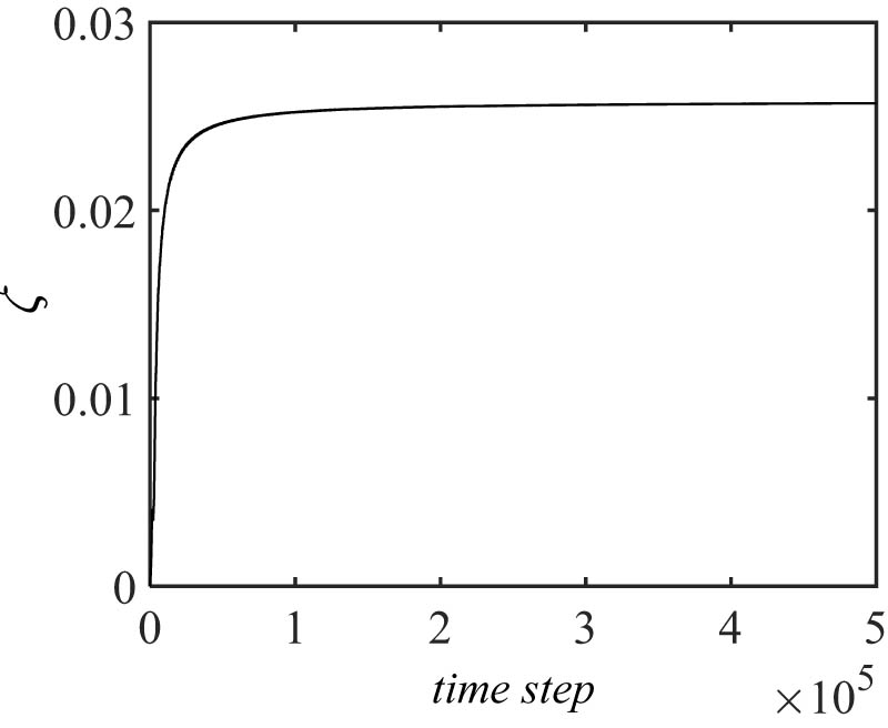
Nonlinear systems can be sensitive to system parameters, and the sensitivity is actually related to the sensitivity index ζ, as ζ measures the shape and displacement variations of two trajectories corresponding to slightly different two system parameters. Considering the same dynamic system governed by Duffing’s equation, for example, a case with B = 11 and K = 0.1, the ζ values are calculated with respect to time t, as shown in Figure 8.

ζ vs time t for a case with B = 11, K = 0.1 based on a small variation of K.
As can be seen from the figure, ζ quickly increases and converges around a value of 0.018, which is significantly larger than that of the ζ values for the periodic case demonstrated previously (numerically 450 times larger in this case). One may conclude, as per the definition of ζ, that this system is sensitive to the parameter K in this case.
Furthermore, in contrast to the periodic cases as shown in Figures 2 and 7, the ζ curve monotonically rises from the initial time period and eventually stabilizes at the large ζ value. The monotonically increasing ζ value indicates that the two curves x = f(t) and y = g(t) increasingly vary and become dramatically different in displacement and shape from the initial time period. Thus, one may state that the ζ curve goes upward from the initial time period as t increases, i.e.,
Figure 9 shows the wave curves, x = f(t) and y = g(t), of the nonlinear system corresponding to two slightly varied K values. As can be seen from the figure, the two curves show chaotic and completely different behavior in terms of displacement and shape. In other words, a slightly varied parameter K causes significant variations in the system response, i.e., the system is sensitive to the parameter K in this case. This agrees with the conclusion provided by the large index ζ.

Displacement curves of x = f(t) and y = g(t), as B = 11, K = 0.1, based on a slight variation of K.
To further demonstrate the sensitivity of the system to parameter K, Figure 10 shows the displacement difference of the two curves x = f(t) and y = g(t), of the nonlinear system corresponding to two slightly varied K values. As can be seen from the figure, the difference of the two curves is not stabilized, much larger than zero, and with much greater variation in terms of displacement and shape.

Displacement difference of the system with a slight variation of system parameter K for a chaotic case of B = 11, K = 0.1.
For this case, a small perturbation in the system parameter B is also examined. Figure 11 shows the ζ values corresponding to a slightly perturbed system parameter B, for the chaotic case of B = 11, K = 0.1. The ζ value for this case is also large, indicating that the system is sensitive to parameter B. Also, one may notice from Figures 8 and 11, ζ–t curves rise quickly from the initial period of time (ζ > 0) and stabilize at large values.

ζ vs time t for a case with B = 11, K = 0.1 based on a very small variation of B.
Figures 8 and 11 show large ζ values. This indicates that the system is sensitive to both the parameters K and B, and the two cases are chaotic. To show the chaotic behavior of the system, before examining the sensitivity of the system to its system parameter, Figure 12 illustrates the corresponding Poincare map.

Poincare map of the system for a chaotic case with B = 11, K = 0.1.
Based on the investigations of the present research, in fact, all the ζ values for chaotic cases are much larger than zero, and the system is sensitive to the system parameters considered. Nonlinear dynamic systems may also have system parameter-dependent sensitivity for quasiperiodic cases. A quasiperiodic case with the Poincare map as shown in Figure 13 can be taken into consideration by employing the index ζ. Again, this is to show a quasiperiodic response of the system before examining the sensitivity of the system to its system parameter.

Poincare map of the system B = 4, K = 0.001.
For this quasiperiodic case with B = 4 and K = 0.001, the corresponding ζ–t diagram is plotted in Figures 14 and 15, in evaluating the sensitivity of the system to the parameters K and B, respectively. As can be seen from the figures, the ζ values converge to large values when the system parameters K and B are slightly varied, respectively.

ζ for a quasi-periodic case with B = 4, K = 0.001 based on a slight variation of K.

ζ for a quasi-periodic case with B = 4, K = 0.001 based on a slight variation of B.
The displacement curve shown in Figure 16 and the displacement different curve in Figure 17 indicate that the two curves with slightly different system parameters indeed cause significant variations in this quasiperiodic case.

Displacement curves of x = f(t) and y = g(t), as B = 4, K = 0.001, based on a slight variation of K.

Displacement difference curve of the system with slight variation of system parameter K for a quasiperiodic case of B = 4, K = 0.001.
From the numerical results shown earlier, it can be seen that the nonlinear system governed by the Duffing’s system is sensitive to system parameters for both chaotic and quasi-periodic cases, as the ζ values of these cases are sufficiently larger than zero and the corresponding ζ curves monotonically rise from their initial time periods. One may therefore conclude that the nonlinear dynamic systems are not sensitive to system parameters if the corresponding sensitivity index ζ is zero or close to zero for numerically determined index ζ. For these insensitive cases, the corresponding ζ curves go monotonically down from the initial time period and asymptotically approach zero. In comparing with the insensitive cases, the nonlinear dynamic systems are sensitive to system parameters when ζ is greater than zero or sufficiently greater than zero if the ζ values and the solutions of the systems are determined numerically. The corresponding ζ–t curves for these cases monotonically rise from the initial time period and eventually stabilize to large ζ values. In other words, chaos and quasi-periodicity are system parameter dependent.
4 Independence of sensitivity index ζ
The sensitivity index ζ may vary with time; however, it is actually independent of the initial conditions of dynamic systems. As discussed previously, ζ measures the sensitivity of a dynamic system to its system parameters, whereas the sensitivity of a system to initial conditions is usually evaluated with tools such as the Lyapunov exponent. It should be noted that dynamic systems with different system parameters are actually different systems, even though the differences can be small. In comparing the system parameter-dependent sensitivity with initial condition-dependent sensitivity, different initial conditions are considered in this research for the cases discussed in the previous section. Also, the initial conditions of a nonlinear dynamic system may affect the ζ values when certain initial conditions are considered. This is also true for the initial condition-dependent sensitivity of a nonlinear system, which may be affected by certain initial conditions of the system. Some of the examples in which Lyapunov exponents give different values when widely spread initial conditions are used [5–7]. Nevertheless, the Lyapunov exponent does not change for the different initial conditions should the same attractor is considered. For all cases discussed in the previous section, the initial displacement and initial velocity used are all set fixed as

ζ vs time t for a case with B = 1, K = 0.4 based on slightly varied K (
In comparing Figures 7 and 18, the difference of the two figures is too small to be identified. This implies that the changes in initial conditions show no effect on the system parameter-dependent sensitivity of the Duffing system considered. The system’s response in this case is periodic, independent of the variation in the initial conditions. For the case with ζ sufficiently larger than zero, using the new initial conditions, Figure 19 shows the ζ curve in comparing with that of Figure 8.

ζ vs time t for a chaotic case with B = 11, K = 0.1 based on a small variation of K (
As can be seen from Figures 8 and 19, the ζ stabilizes to two values very close to each other. Nevertheless, both ζ values are sufficiently larger than zero. In other words, the chaotic behavior of the system or the parameter-dependent sensitivity of the system does not change regardless of the variation in the initial conditions. For comparing the quasiperiodic case as shown in Figure 14, a ζ curve is plotted in Figure 20 for the same case but the different initial conditions.

ζ for a quasiperiodic case with B = 4, K = 0.001 based on the slight variation of K (
Comparing Figures 14 and 20, the difference in converged ζ values is small. Nevertheless, the two converged ζ values are both high. This implies that the changes in initial conditions have no effect on the fact that the system is quasiperiodic. One may therefore state that the initial conditions have a limited effect on the sensitivity of the system to its system parameters, although different initial conditions may result with different ζ values. In conclusion, system parameter-dependent sensitivity of a nonlinear system is independent of the system’s initial condition-dependent sensitivity. Chaos, for example, is usually described as sensitive to initial conditions. With the aforementioned descriptions, chaos together with quasi-periodicity can be additionally described as sensitive to system parameters.
In numerically determining the sensitivity index, the system parameters are perturbed at a variation of 1% of the considered. To show the influence of variation values on the sensitivity indexes, the figures of percent variation vs sensitivity indexes are plotted in Figures 21 and 22. Figure 21 indicates the ζ values at different variations of K when K = 0.4, B = 1 (periodic case). With the increased perturbation value from 1 to 3%, the ζ value increase but still show a small value (1.6 × 10⁻⁵) of the sensitivity index, which indicates a periodic case. However, the figure also illustrates that the ζ value increases with the increase of the parameter variation. Nevertheless, a smaller variation is favorable, in considering that ζ should be zero theoretically for a periodic case.
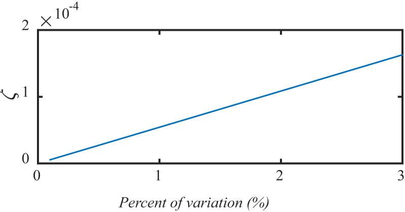
ζ for different variations of K at the case K = 0.4, B = 1, with

ζ for different variations of K at the case K = 0.1, B = 11 with
Figure 22 indicates the ζ values at different variation values of K when K = 0.1 and B = 11. This is a chaotic case as discussed previously. As can be seen from the figure, the ζ values vary with the perturbed values varying from 1 to 3% for the parameter K. However, ζ shows a positive value at all the percent of variation. It can be concluded that even though the change of variations may slightly change the ζ values; it will not change the characteristics of the system.
To show the efficiency of the proposed method, the Van der Pol system [35] is also applied as expressed:
A periodic case with A = 0.5, Ω = 1, μ = 1 is first selected with the corresponding Poincare map as shown in Figure 23. Based on the proposed approach as described earlier, with a perturbation of parameter A and μ, ζ are calculated as indicated in Figures 24 and 25, respectively. It can be seen that for this considered periodic case, for both two parameters, the ζ values are approaching to be 0, which shows agreement with Duffing’s system. While for a quasi-periodic case when A = 5, μ = 3, Ω = 1.78 [35], as indicated in Figure 26, ζ values to system parameters A and μ are plotted in Figures 27 and 28, respectively. Analogous with Duffing’s system, the ζ values for quasi-periodic case are also positive, indicating the efficiency of the proposed approach in quantifying for nonlinear systems.

Poincare map of the system A = 0.5, μ = 1, Ω = 1.

ζ for a periodic case with A = 0.5, μ = 1 in the Van der Pol system based on the slight variation of A.

ζ for a periodic case with A = 0.5, μ = 1 in the Van der Pol system based on the slight variation of μ.

Poincare map of the system A = 5, μ = 3, Ω = 1.78.

ζ for a periodic case with A = 5, μ = 3 in the Van der Pol system based on the slight variation of A.

ζ for a periodic case with A = 5, μ = 3 in the Van der Pol system based on the slight variation of μ.
5 Sensitive regions of nonlinear dynamic system to its system parameters
As a single value index, ζ can be conveniently employed to evaluate the sensitivity of a nonlinear dynamic system to one or more of its system parameters over a wide range. A diagram showing regions of system parameter-dependent sensitivity of a nonlinear system can therefore be constructed, for desired system parameters and desired ranges of the system parameters. For the nonlinear dynamics system governed by the Duffing’s equation considered, the sensitivity of the system to system parameter K is examined by implementing the sensitive index ζ. Figure 29 shows a sensitivity region diagram constructed over a range of system parameters: 0 ≤ B ≤ 25 and 0 ≤ K ≤ 0.8. There are 10,000 points shown in the diagram, which represents 10,000 cases examined with the index ζ.

Sensitivity of the Duffing’s system to system parameter K over the ranges of system parameters: 0 ≤ B ≤ 25 and 0 ≤ K ≤ 0.8.
In Figure 29, different colors represent different values of ζ. The blue areas in the figure indicate regions where the system is not sensitive to parameter K (i.e., ζ is zero as shown in the color bar legend to the right of the figure). These areas are the periodic regions of the system. The other colors indicate regions in which the system is sensitive to parameter K, i.e., the chaotic or quasiperiodic areas of the responses of the system. The higher ζ value implies higher sensitivity of the dynamic system to parameter K, or more severe displacement and velocity changes of the system’s response to the slight but identical perturbation of the parameter K.
One of the advantages of such sensitivity region diagram is its convenience for studying transitional changes in the dynamic system with respect to continuous changes in system parameters. To illustrate this, a Poincare map and a bifurcation diagram of the Duffing system are shown in Figures 30 and 31, respectively. The Poincare maps of three cases taken from the sensitivity region diagram are plotted in Figure 30. The black stars in the figure represent the Poincare map for a case of K = 0.1 and B = 4 with ζ equal to 0. The red points for a chaotic case of K = 0.1 and B = 9.5 with ζ equal to 0.045, and the blue points indicate another chaotic case of K = 0.1 and B = 25 with ζ equal to 0.025. As shown in Figure 22, the points for a larger ζ value case are more dispersive than that of a small ζ case, even though they are both chaotic. In the bifurcation diagram shown in Figure 23, one may also see the difference in the system’s chaotic responses for B = 9.5 and B = 25 while maintaining the same K value of 0.1. This also implies that the degree of sensitivity increases as the ζ value increases.

Poincare maps for three cases taken from the sensitivity areas of the region diagram (ζ = 0; ζ = 0.025; ζ = 0.045).

Bifurcation diagram of the Duffing’s system, K = 0.1.
A region diagram of the Duffing’s system is also constructed for the sensitivity of the system to parameter B, as shown in Figure 32.

Sensitivity of the Duffing’s system to system parameter B over the ranges of system parameters: 0 ≤ B ≤ 25 and 0 ≤ K ≤ 0.8.
The two figures of Figures 29 and 32 are similar in most areas, indicating similar sensitivities of the system to the two system parameters B and K and reflecting the inherent nature of the nonlinear system. Nevertheless, differences between the two figures are evident. This implies that different system parameters may have different effects on the system parameter-dependent sensitivity of the nonlinear systems. With fixed initial conditions and parameter values, the different sensitivities of the nonlinear system can be shown with respect to different system parameters. Two cases are taken from the two region diagrams Figures 29 and 32, respectively, and are shown in Figures 33 and 34, respectively. As shown in Figures 33 and 34 with the same K and B values, the sensitivities of the Duffing’s system to parameters K and B are quite different. Figure 33 indicates a chaotic case with K = 0.1, B = 9.5, based on a slight perturbation of B.
ζ for a case, K = 0.1, B = 9.5, based on a slight variation of B.

ζ for a periodic case, under the identical conditions as that of Figure 32, K = 0.1, B = 9.5, based on a slight variation of K.
Under identical conditions, Figure 34 shows the ζ curve of the system corresponding to a slight variation of parameter K. As can be seen from Figure 34, the stabilized ζ is zero. In contrast to that of Figure 34, this is a periodic case, which is not sensitive to the parameter K.
As presented previously, system parameter-dependent sensitivity is different from the initial condition-dependent sensitivity. The region diagrams of the identical Duffing’s system can be found in the literature, for its sensitivity to initial conditions [32,34]. Interested readers may compare the similarities and differences of these diagrams and see the correlation between the initial condition-dependent sensitivity and the system parameter-dependent sensitivity of identical nonlinear dynamic systems. The two types of diagrams for the Duffing’s system show significant similarities, reflecting the inherent or intrinsic nature of the nonlinear system.
6 Conclusions
Sensitivity analysis of nonlinear dynamic systems focuses mainly on initial condition-dependent sensitivities. To the best of our knowledge, there is little work in qualitative evaluation or analysis of system parameter-dependent sensitivity of nonlinear dynamic systems, even though such study is important and practically significant in nonlinear dynamics. The present research develops a theoretical measure called the sensitive index (ζ) for quantitatively measuring the sensitivity dependence of nonlinear systems on system parameters. The application of ζ is shown in analyzing a nonlinear system governed by the Duffing’s equation. With the findings of this research, the following conclusions can be drawn.
Chaotic and quasiperiodic systems are sensitive to system parameters, in addition to their sensitivities to initial conditions, and the parameter-dependent sensitivity can be quantified by the Sensitivity Index ζ. Both system parameter and initial condition-dependent sensitivities represent the inherent or intrinsic nature of a nonlinear system.
The sensitivity index gives the degree of sensitivity of a nonlinear dynamic system to its system parameters. Theoretically, a system is insensitive to its system parameter(s) when ζ is zero, and a system is sensitive to the system parameter(s) when ζ is greater than zero.
The sensitivity index ζ is easy to use, and the application of the index shows its simplicity and effectiveness.
For sensitive cases of nonlinear systems; ζ–t curve goes upward, whereas
For the insensitive case of nonlinear systems, ζ–t curve goes downward, whereas
Different system parameter has a different effect on the sensitivity of nonlinear systems to their system parameters. With fixed system parameters and initial conditions, a given nonlinear system can be sensitive to one parameter but not necessarily sensitive to the other parameters.
The single value sensitivity index ζ enables the construction of sensitivity region diagrams, which illustrate sensitive and insensitive regions together with the degree of sensitivities of a nonlinear system to its parameters, across different system parameters. Such a diagram is a useful tool for researchers and engineers to visualize system parameter dependency and helps to avoid designing nonlinear systems with unwanted responses.
-
Funding information: This research was funded by National Natural Science Foundation of China (52278537, 52408558), Fujian Provincial Natural Science Foundation (2022J011251), and High-level talent program of Xiamen University of Technology (YKJ23006R).
-
Author contributions: Methodology: Dandan Xia, Liming Dai; validation: Dandan Xia, Liming Dai; formal analysis, Dandan Xia, Liming Dai; investigation: Dandan Xia, Liming Dai; writing - original draft: Dandan Xia. All authors have accepted responsibility for the entire content of this manuscript and approved its submission.
-
Conflict of interest: The authors state no conflict of interest.
-
Data availability statement: The datasets generated during and/or analyzed during the current study are available from the corresponding author on reasonable request.
References
[1] Brandstater A, Swinney HL. Distinguishing low-dimensional chaos from random noise in a hydrodynamic experiment. Fluctuations and sensitivity in nonequilibrium. Vol. 1. Berlin, Heidelberg: Springer Proceedings in Physics; 1983. p. 166–71.10.1007/978-3-642-46508-6_17Search in Google Scholar
[2] Malraison B, Atten P. Chaotic behavior of instability due to unipolar ion injection in a dielectric liquid. Phys Rev Lett. 1982;49:723–6.10.1103/PhysRevLett.49.723Search in Google Scholar
[3] Machado LG, Lagoudas DC, Savi MA. Lyapunov exponents estimation for hysteretic systems. Int J Solids Struct. 2009;46:1269–86.10.1016/j.ijsolstr.2008.09.013Search in Google Scholar
[4] Wan H, Ren W, Todd D. Arbitrary polynomial chaos expansion method for uncertainty quantification and global sensitivity analysis in structural dynamics. Mech Syst Signal Process. 2020;142:106732.10.1016/j.ymssp.2020.106732Search in Google Scholar
[5] Wolf A, Swift JB, Swinney HL, Vastano JA. Determining Lyapunov exponents from a time series. Phys D. 1985;16:285–317.10.1016/0167-2789(85)90011-9Search in Google Scholar
[6] Dai L, Singh MC. An analytical and numerical method for solving linear and nonlinear vibration problems. Int J Solids Struct. 1997;34:2709–31.10.1016/S0020-7683(96)00169-2Search in Google Scholar
[7] Dai L, Wang G. Implementation of periodicity ratio in analyzing nonlinear dynamic systems: A comparison with Lyapunov exponent. J Comput Nonlinear Dyn. 2008;3:011006.1–9.10.1115/1.2802581Search in Google Scholar
[8] Dai L, Xia D, Chen C. An algorithm for diagnosing nonlinear characteristics of dynamic systems with the integrated periodicity ratio and Lyapunov exponent methods. Commun Nonlinear Sci Numer Simul. 2019;73:92–109.10.1016/j.cnsns.2019.01.029Search in Google Scholar
[9] Christian S, Gustavo D. Identification of deterministic chaos by an information-theoretic measure of the sensitive dependence on the initial conditions. Phys D. 1997;110:173–81.10.1016/S0167-2789(97)00127-9Search in Google Scholar
[10] Srinivasan M. Chaos in a soda can: Non-periodic rocking of upright cylinders with sensitive dependence on initial conditions. Mech Res Commun. 2009;36:722–7.10.1016/j.mechrescom.2009.03.008Search in Google Scholar
[11] Collins M, Allen MR. Assessing the relative roles of initial and boundary conditions in inter-annual to decadal climate predictability. J Clim. 2002;15:3104–9.10.1175/1520-0442(2002)015<3104:ATRROI>2.0.CO;2Search in Google Scholar
[12] Lorenz EN. The physical bases of climate and climate modeling. Clim Predict. 1975;16:132–6. WMO.Search in Google Scholar
[13] Zhang F, Odins AM, Nielsen-Gammon JW. Mesoscale predictability of an extreme warm-season precipitation event. Weather Forecast. 2006;21:149–66.10.1175/WAF909.1Search in Google Scholar
[14] Zhang FQ, Snyder C, Rotunno R. Mesoscale predictability of the “surprise” snowstorm of 24-25 January 2000. Mon Weather Rev. 2002;130:1617–32.10.1175/1520-0493(2002)130<1617:MPOTSS>2.0.CO;2Search in Google Scholar
[15] Zhu HY, Thorpe A. Predictability of extra-tropical cyclones: The influence of initial-condition and model uncertainties. J Atmos Sci. 2006;63:1483–97.10.1175/JAS3688.1Search in Google Scholar
[16] Christophe A, Biau G, Cadrec B. On Lyapunov exponent and sensitivity. J Math Anal Appl. 2004;290:395–404.10.1016/j.jmaa.2003.10.029Search in Google Scholar
[17] Adelman HM, Haftka RT. Sensitivity analysis of discrete structural systems. AIAAJ. 1986;24:823–32.10.2514/3.48671Search in Google Scholar
[18] Bettencourt LMA, Cintron-Arias A, Kaiser DI, Castillo-Chavez C. The power of a good idea: Quantitative modeling of the spread of ideas from epidemiological models. Physica A. 2006;364:513–36.10.1016/j.physa.2005.08.083Search in Google Scholar
[19] Blower SM, Dowlatabadi H. Sensitivity and uncertainty analysis of complex models of disease transmission: An HIV model as an example. Intern Stat Rev. 1994;62:229–43.10.2307/1403510Search in Google Scholar
[20] Matyja K. Standard dynamic energy budget model parameter sensitivity. Ecol Model. 2023;478:11304.10.1016/j.ecolmodel.2023.110304Search in Google Scholar
[21] Farmer JD. Sensitive dependence on parameters in nonlinear dynamics. Phys Rev Lett. 1985;55:351.10.1103/PhysRevLett.55.351Search in Google Scholar
[22] Haro Sandoval E, Anstett-Collin F, Basset M. Sensitivity study of dynamic systems with polynomial chaos. Reliab Eng Syst Saf. 2012;104:15–26.10.1016/j.ress.2012.04.001Search in Google Scholar
[23] Soll T, Pulch R. Sample selection based on sensitivity analysis in parameterized model order reduction. J Comput Appl Math. 2017;316:271–86.10.1016/j.cam.2016.09.046Search in Google Scholar
[24] Roland P, Narayan A. Sensitivity analysis of random linear dynamical systems using quadratic outputs. J Comput Appl Math. 2019;387:112491.10.1016/j.cam.2019.112491Search in Google Scholar
[25] Rocco FD, Cacuci DG. Sensitivity and uncertainty analysis of a reduced-order model of nonlinear BWR dynamics: I. Forward sensitivity analysis. Ann Nucl Energy. 2020;148:107738.10.1016/j.anucene.2020.107738Search in Google Scholar
[26] Ballaben JS, Guzman AM, Rosales MB. Nonlinear dynamics of guyed masts under wind load: Sensitivity to structural parameters and load models. J Wind Eng Ind Aerodyn. 2017;169:128–38.10.1016/j.jweia.2017.07.012Search in Google Scholar
[27] Medeiros ES, Caldas IL, Baptistab MS. Sensitive dependence on parameters of continuous-time nonlinear dynamical systems. Chaos Solitons Fractals. 2017;99:16–9.10.1016/j.chaos.2017.03.043Search in Google Scholar
[28] Wilkins AK, Tidor B, White J, Barton P. Sensitivity analysis for oscillating dynamical systems. SIAM J Sci Comput. 2009;31(4):2706–32.10.1137/070707129Search in Google Scholar PubMed PubMed Central
[29] Lajimi SAM, Heppler GR, Abdel-Rahman EM. A parametric study of the nonlinear dynamics and sensitivity of a beam-rigid body microgyroscope. Commun Nonlinear Sci Numer Simul. 2017;50:180–92.10.1016/j.cnsns.2017.02.016Search in Google Scholar
[30] Yan D, Chen Q, Zheng Y, Liu W. Parameter sensitivity and dynamic characteristic analysis of bulb hydro generating unit with shaft crack fault. Mech Syst Signal Process. 2021;158:107732.10.1016/j.ymssp.2021.107732Search in Google Scholar
[31] Fan G, Li X, Zhang R. Global sensitivity analysis on temperature-dependent parameters of a reduced-order electrochemical model and robust state-of-charge estimation at different temperatures. Energy. 2021;223:12002.10.1016/j.energy.2021.120024Search in Google Scholar
[32] Dai L. Nonlinear dynamics of piecewise constant systems and implementation of piecewise constant arguments. New Jersey: World Scientific Publishing Co; 2008.10.1142/9789812818515Search in Google Scholar
[33] Akanksha V, Wojciech S, Pramod KY. The numerical solution of nonlinear fractional Lienard and Duffing equations using orthogonal perceptron. Symmetry. 2023;15:1753.10.3390/sym15091753Search in Google Scholar
[34] Ueda Y. Steady motions exhibited by Duffing’s equation: A picture book of regular and chaotic motions. In: Holmes PJ, editor. New approaches to nonlinear problems in dynamics. Philadelphia: SIAM; 1980. p. 311–22.Search in Google Scholar
[35] Marios T. Theoretical and numerical study of the Van der Pol equation [D]. Thessaloniki, Greece: Aristotle University of Thessaloniki; 2006.Search in Google Scholar
© 2025 the author(s), published by De Gruyter
This work is licensed under the Creative Commons Attribution 4.0 International License.
Articles in the same Issue
- Research Articles
- Generalized (ψ,φ)-contraction to investigate Volterra integral inclusions and fractal fractional PDEs in super-metric space with numerical experiments
- Solitons in ultrasound imaging: Exploring applications and enhancements via the Westervelt equation
- Stochastic improved Simpson for solving nonlinear fractional-order systems using product integration rules
- Exploring dynamical features like bifurcation assessment, sensitivity visualization, and solitary wave solutions of the integrable Akbota equation
- Research on surface defect detection method and optimization of paper-plastic composite bag based on improved combined segmentation algorithm
- Impact the sulphur content in Iraqi crude oil on the mechanical properties and corrosion behaviour of carbon steel in various types of API 5L pipelines and ASTM 106 grade B
- Unravelling quiescent optical solitons: An exploration of the complex Ginzburg–Landau equation with nonlinear chromatic dispersion and self-phase modulation
- Perturbation-iteration approach for fractional-order logistic differential equations
- Variational formulations for the Euler and Navier–Stokes systems in fluid mechanics and related models
- Rotor response to unbalanced load and system performance considering variable bearing profile
- DeepFowl: Disease prediction from chicken excreta images using deep learning
- Channel flow of Ellis fluid due to cilia motion
- A case study of fractional-order varicella virus model to nonlinear dynamics strategy for control and prevalence
- Multi-point estimation weldment recognition and estimation of pose with data-driven robotics design
- Analysis of Hall current and nonuniform heating effects on magneto-convection between vertically aligned plates under the influence of electric and magnetic fields
- A comparative study on residual power series method and differential transform method through the time-fractional telegraph equation
- Insights from the nonlinear Schrödinger–Hirota equation with chromatic dispersion: Dynamics in fiber–optic communication
- Mathematical analysis of Jeffrey ferrofluid on stretching surface with the Darcy–Forchheimer model
- Exploring the interaction between lump, stripe and double-stripe, and periodic wave solutions of the Konopelchenko–Dubrovsky–Kaup–Kupershmidt system
- Computational investigation of tuberculosis and HIV/AIDS co-infection in fuzzy environment
- Signature verification by geometry and image processing
- Theoretical and numerical approach for quantifying sensitivity to system parameters of nonlinear systems
- Chaotic behaviors, stability, and solitary wave propagations of M-fractional LWE equation in magneto-electro-elastic circular rod
- Dynamic analysis and optimization of syphilis spread: Simulations, integrating treatment and public health interventions
- Visco-thermoelastic rectangular plate under uniform loading: A study of deflection
- Threshold dynamics and optimal control of an epidemiological smoking model
- Numerical computational model for an unsteady hybrid nanofluid flow in a porous medium past an MHD rotating sheet
- Regression prediction model of fabric brightness based on light and shadow reconstruction of layered images
- Dynamics and prevention of gemini virus infection in red chili crops studied with generalized fractional operator: Analysis and modeling
- Qualitative analysis on existence and stability of nonlinear fractional dynamic equations on time scales
- Fractional-order super-twisting sliding mode active disturbance rejection control for electro-hydraulic position servo systems
- Analytical exploration and parametric insights into optical solitons in magneto-optic waveguides: Advances in nonlinear dynamics for applied sciences
- Bifurcation dynamics and optical soliton structures in the nonlinear Schrödinger–Bopp–Podolsky system
- User profiling in university libraries by combining multi-perspective clustering algorithm and reader behavior analysis
- Exploring bifurcation and chaos control in a discrete-time Lotka–Volterra model framework for COVID-19 modeling
- Review Article
- Haar wavelet collocation method for existence and numerical solutions of fourth-order integro-differential equations with bounded coefficients
- Special Issue: Nonlinear Analysis and Design of Communication Networks for IoT Applications - Part II
- Silicon-based all-optical wavelength converter for on-chip optical interconnection
- Research on a path-tracking control system of unmanned rollers based on an optimization algorithm and real-time feedback
- Analysis of the sports action recognition model based on the LSTM recurrent neural network
- Industrial robot trajectory error compensation based on enhanced transfer convolutional neural networks
- Research on IoT network performance prediction model of power grid warehouse based on nonlinear GA-BP neural network
- Interactive recommendation of social network communication between cities based on GNN and user preferences
- Application of improved P-BEM in time varying channel prediction in 5G high-speed mobile communication system
- Construction of a BIM smart building collaborative design model combining the Internet of Things
- Optimizing malicious website prediction: An advanced XGBoost-based machine learning model
- Economic operation analysis of the power grid combining communication network and distributed optimization algorithm
- Sports video temporal action detection technology based on an improved MSST algorithm
- Internet of things data security and privacy protection based on improved federated learning
- Enterprise power emission reduction technology based on the LSTM–SVM model
- Construction of multi-style face models based on artistic image generation algorithms
- Research and application of interactive digital twin monitoring system for photovoltaic power station based on global perception
- Special Issue: Decision and Control in Nonlinear Systems - Part II
- Animation video frame prediction based on ConvGRU fine-grained synthesis flow
- Application of GGNN inference propagation model for martial art intensity evaluation
- Benefit evaluation of building energy-saving renovation projects based on BWM weighting method
- Deep neural network application in real-time economic dispatch and frequency control of microgrids
- Real-time force/position control of soft growing robots: A data-driven model predictive approach
- Mechanical product design and manufacturing system based on CNN and server optimization algorithm
- Application of finite element analysis in the formal analysis of ancient architectural plaque section
- Research on territorial spatial planning based on data mining and geographic information visualization
- Fault diagnosis of agricultural sprinkler irrigation machinery equipment based on machine vision
- Closure technology of large span steel truss arch bridge with temporarily fixed edge supports
- Intelligent accounting question-answering robot based on a large language model and knowledge graph
- Analysis of manufacturing and retailer blockchain decision based on resource recyclability
- Flexible manufacturing workshop mechanical processing and product scheduling algorithm based on MES
- Exploration of indoor environment perception and design model based on virtual reality technology
- Tennis automatic ball-picking robot based on image object detection and positioning technology
- A new CNN deep learning model for computer-intelligent color matching
- Design of AR-based general computer technology experiment demonstration platform
- Indoor environment monitoring method based on the fusion of audio recognition and video patrol features
- Health condition prediction method of the computer numerical control machine tool parts by ensembling digital twins and improved LSTM networks
- Establishment of a green degree evaluation model for wall materials based on lifecycle
- Quantitative evaluation of college music teaching pronunciation based on nonlinear feature extraction
- Multi-index nonlinear robust virtual synchronous generator control method for microgrid inverters
- Manufacturing engineering production line scheduling management technology integrating availability constraints and heuristic rules
- Analysis of digital intelligent financial audit system based on improved BiLSTM neural network
- Attention community discovery model applied to complex network information analysis
- A neural collaborative filtering recommendation algorithm based on attention mechanism and contrastive learning
- Rehabilitation training method for motor dysfunction based on video stream matching
- Research on façade design for cold-region buildings based on artificial neural networks and parametric modeling techniques
- Intelligent implementation of muscle strain identification algorithm in Mi health exercise induced waist muscle strain
- Optimization design of urban rainwater and flood drainage system based on SWMM
- Improved GA for construction progress and cost management in construction projects
- Evaluation and prediction of SVM parameters in engineering cost based on random forest hybrid optimization
- Museum intelligent warning system based on wireless data module
- Optimization design and research of mechatronics based on torque motor control algorithm
- Special Issue: Nonlinear Engineering’s significance in Materials Science
- Experimental research on the degradation of chemical industrial wastewater by combined hydrodynamic cavitation based on nonlinear dynamic model
- Study on low-cycle fatigue life of nickel-based superalloy GH4586 at various temperatures
- Some results of solutions to neutral stochastic functional operator-differential equations
- Ultrasonic cavitation did not occur in high-pressure CO2 liquid
- Research on the performance of a novel type of cemented filler material for coal mine opening and filling
- Testing of recycled fine aggregate concrete’s mechanical properties using recycled fine aggregate concrete and research on technology for highway construction
- A modified fuzzy TOPSIS approach for the condition assessment of existing bridges
- Nonlinear structural and vibration analysis of straddle monorail pantograph under random excitations
- Achieving high efficiency and stability in blue OLEDs: Role of wide-gap hosts and emitter interactions
- Construction of teaching quality evaluation model of online dance teaching course based on improved PSO-BPNN
- Enhanced electrical conductivity and electromagnetic shielding properties of multi-component polymer/graphite nanocomposites prepared by solid-state shear milling
- Optimization of thermal characteristics of buried composite phase-change energy storage walls based on nonlinear engineering methods
- A higher-performance big data-based movie recommendation system
- Nonlinear impact of minimum wage on labor employment in China
- Nonlinear comprehensive evaluation method based on information entropy and discrimination optimization
- Application of numerical calculation methods in stability analysis of pile foundation under complex foundation conditions
- Research on the contribution of shale gas development and utilization in Sichuan Province to carbon peak based on the PSA process
- Characteristics of tight oil reservoirs and their impact on seepage flow from a nonlinear engineering perspective
- Nonlinear deformation decomposition and mode identification of plane structures via orthogonal theory
- Numerical simulation of damage mechanism in rock with cracks impacted by self-excited pulsed jet based on SPH-FEM coupling method: The perspective of nonlinear engineering and materials science
- Cross-scale modeling and collaborative optimization of ethanol-catalyzed coupling to produce C4 olefins: Nonlinear modeling and collaborative optimization strategies
- Unequal width T-node stress concentration factor analysis of stiffened rectangular steel pipe concrete
- Special Issue: Advances in Nonlinear Dynamics and Control
- Development of a cognitive blood glucose–insulin control strategy design for a nonlinear diabetic patient model
- Big data-based optimized model of building design in the context of rural revitalization
- Multi-UAV assisted air-to-ground data collection for ground sensors with unknown positions
- Design of urban and rural elderly care public areas integrating person-environment fit theory
- Application of lossless signal transmission technology in piano timbre recognition
- Application of improved GA in optimizing rural tourism routes
- Architectural animation generation system based on AL-GAN algorithm
- Advanced sentiment analysis in online shopping: Implementing LSTM models analyzing E-commerce user sentiments
- Intelligent recommendation algorithm for piano tracks based on the CNN model
- Visualization of large-scale user association feature data based on a nonlinear dimensionality reduction method
- Low-carbon economic optimization of microgrid clusters based on an energy interaction operation strategy
- Optimization effect of video data extraction and search based on Faster-RCNN hybrid model on intelligent information systems
- Construction of image segmentation system combining TC and swarm intelligence algorithm
- Particle swarm optimization and fuzzy C-means clustering algorithm for the adhesive layer defect detection
- Optimization of student learning status by instructional intervention decision-making techniques incorporating reinforcement learning
- Fuzzy model-based stabilization control and state estimation of nonlinear systems
- Optimization of distribution network scheduling based on BA and photovoltaic uncertainty
- Tai Chi movement segmentation and recognition on the grounds of multi-sensor data fusion and the DBSCAN algorithm
- Special Issue: Dynamic Engineering and Control Methods for the Nonlinear Systems - Part III
- Generalized numerical RKM method for solving sixth-order fractional partial differential equations