Computational investigation of tuberculosis and HIV/AIDS co-infection in fuzzy environment

Harshita Kaushik; Vijai Shanker Verma; Ram Singh; Sonal Jain; Salah Boulaaras

doi:10.1515/nleng-2025-0131

Article Open Access

Computational investigation of tuberculosis and HIV/AIDS co-infection in fuzzy environment

Harshita Kaushik , Vijai Shanker Verma , Ram Singh , Sonal Jain and Salah Boulaaras

Published/Copyright: June 2, 2025

Published by

Become an author with De Gruyter Brill

Submit Manuscript Author Information

From the journal Nonlinear Engineering Volume 14 Issue 1

Abstract

Tuberculosis (TB) and human immunodeficiency virus (HIV)/acquired immunodeficiency virus (AIDS) have a fatal bidirectional connection with a significant global epidemic overlap. People living with HIV-positive are over 30 times more likely than HIV-negative people to develop TB and active TB causes the chronic immunological activation, which accelerates HIV/AIDS disease development. This gives computational investigation of a TB and HIV/AIDS co-infection in fuzzy environment. The application of fuzzy theory aids in addressing the difficulties associated with measuring uncertainty in mathematical representations of the diseases. Here, the fuzzy reproduction number and fuzzy equilibrium points are obtained by using a model relevant to a specific group described by the triangular membership function. Two numerical techniques, namely, forward Euler’s method and Runge–Kutta method, are developed within a fuzzy framework to address the model. We have also employed the non-standard finite difference scheme, which ensures the preservation of the essential properties such as positivity, convergence, and consistency. Numerical simulations are also conducted to illustrate the applicability of the developed technique.

Keywords: tuberculosis and HIV/AIDS; fuzzy environment; forward Euler’s method; Runge–Kutta method; finite difference scheme; numerical methods; mathematical model

1 Introduction

In order to comprehend the transmission dynamics of diseases within human populations, mathematical modeling of infectious diseases makes use of numerous mathematical and techniques. The objectives of study of the disease dynamics are to understand patterns of transmission, predict how an epidemic will emerge in the future, evaluate the efficacy of control measures, and provide guidance for public health initiatives. Mathematical models can incorporate a variety of factors, including population demographics, illness characteristics, transmission pathways, and intervention strategies, to simulate and evaluate the evolution of infectious diseases. These models can help researchers and policymakers make informed decisions about mitigating, controlling, and eradicating the diseases. Mathematical modeling is used in epidemiology to explain how illnesses spread and affect communities [1–5]. Epidemiological models facilitate a more profound understanding of the transmission of the disease and its preventive strategies [6]. An extensive array of epidemiological models were created, evaluated, and employed qualitatively and quantitatively to investigate a broad spectrum of infections caused by various types of pathogens. Many traditional schemes, such as Euler’s method, Euler’s improved method, Runge–Kutta method, and related techniques, may face challenges such chaos, oscillations, and false steady states. Another way to get around these numerical instabilities is to build schemes with the non-standard finite-difference (NSFD) approach [7,8]. This approach makes it possible to prevent the problems stated above and provides increased stability when performing numerical calculations. This technique, pioneered by Mickens [9], has resulted in the development of new numerical schemes that preserve essential properties such as stability, positivity, and boundedness. In order to improve our comprehension of transmission dynamics and disease control, a multitude of models have been created and investigated using a variety of approaches [10]. In 1965, Zadeh developed the concept of fuzzy theory [9,11,12]. Fuzzy theory is essential to mathematical modeling, because it provides a way to deal with unclear or ambiguous data inside a mathematical framework. All variables are assumed to be precisely measured or calculated in conventional mathematical models. Taking into account, we have made our interest focusing on co-infection dynamics of human immunodeficiency virus (HIV)/acquired immunodeficiency virus (AIDS) and tuberculosis (TB) [13].

HIV has emerged as one of the leading causes of death and misery around the whole world. In 2019, HIV ranked as the eleventh biggest cause of disease burden worldwide [11]. HIV is the ninth and second major cause of disease worldwide in the age categories 10–24 years and 25–49 years, respectively. This finding highlights the ongoing problem of dealing with HIV globally [14]. The world health organization worldwide HIV program [15] recognizes HIV as a significant issue in global public health, since it has killed about 36.3 million lives. In 2020, the program anticipates 37.7 million individuals living with HIV, 1.5 million newly infected in the previous year, and 0.8 million persons globally died from HIV-related causes.

HIV disrupts functioning of immune system of human body by targeting CD4+ T-cells, which protect the host from infections/pathogens [16]. HIV targets and kills these cells, making it more difficult for the body to fight off additional infections. HIV is mostly transmitted through unprotected sexual contact, infected needles, blood transfusions, and lactation [17]. Heterosexual interaction continues to be the most common way that HIV is spread [18]. HIV can spread depending on how infectious the partner is. In the advanced stages of the illness, higher virus loads are linked to an increased risk of transmission [19]. As the HIV progresses, it is commonly referred to as AIDS. Preventive measures including loyalty, protection, and abstinence are the major ways to fight the disease, even though they cannot be stopped forever [20]. These strategies mostly depend on the level of behavioral change observed in the community and the anti-retroviral treatment (ART) administered to infected patients [21]. ART medication increases life expectancy, improves health, and greatly lowers the risk of HIV transmission.

Mycobacterium tuberculosis bacteria causes the TB. It is among the earliest diseases that have been identified, and it is brought on by inhaling aerosolized bacilli of the causing agent. It is acquired by sharing a closed, communal space with contagious individuals. Lung infections from TB are common. However, it can also infect other tissues and organs. To treat TB, a variety of anti-TB medications are taken. Every year, millions of individuals still develop TB [22]. Approximately 25% of the population has latent TB, which is the infection that has not yet resulted in illness [23]. Latently infected persons cannot spread TB. Latent TB infections frequently do not result in TB disease. Some of them become infected with TB when their immune systems deteriorate for other reasons. Approximately 10 million individuals are affected, comprising around 5.6 million men, 3.2 million women, and 1.2 million children. In 2017, 6.4 million new cases worldwide were reported to national authorities; this amounts to only 64% of the 10 million new cases that were expected. Underreporting of detected cases and underdiagnosis cases combine to cause the discrepancy between the number of newly reported cases that are actually reported and the estimated number of cases [23].

Using a comparative table in research, such as the one presented in “A GPT-Based Approach for Sentiment Analysis and Bakery Rating Prediction” by Magdaleno et al., is crucial for clearly presenting differences between methodologies, such as a fuzzy model versus deterministic models. Comparative tables allow researchers to systematically showcase key performance metrics (e.g., accuracy, flexibility, robustness) in an organized format, highlighting the advantages and trade-offs of each approach [24–26].

The fuzzy model offers significant advantages over deterministic models and previous studies by better handling uncertainty and imprecision in data. Unlike deterministic models that rely on precise inputs and outputs, fuzzy models can manage ambiguous or incomplete information through degrees of membership, resulting in more adaptable and realistic predictions in complex, real-world scenarios. Studies comparing the two approaches often show that fuzzy models outperform deterministic ones in environments where uncertainty, variability, or linguistic ambiguity exists, making them more flexible and robust for decision-making in fields such as engineering, economics, and control systems. This flexibility provides more accurate results where deterministic models may struggle with oversimplification or rigid assumptions.

The various co-dynamics of numerous illnesses are studied by several epidemiologists [27–31]. Various techniques have been used to reduce the effect of co-infections on the host’s health and the spread of diseases in the human society. Numerous investigations have been carried out on the co-dynamics of the TB with other illnesses. Depending on the goal and direction of the research; various models of TB and HIV/AIDS co-infections have been studied earlier [32]. This study examines the spatial and temporal patterns of COVID-19 spread by leveraging a self-organizing neural network for spatial mapping and a fuzzy fractal approach to capture temporal dynamics across various countries. Based on self-organization, and neural networks, countries with a similar COVID-19 spread can be spatially categorized; this way, we may assess whether countries have comparable characteristics. As a result, similar tactics for preventing virus spread may be advantageous. Furthermore, a fuzzy fractal technique is employed for the temporal analysis of time-series trends of the researched countries [33]. Fuzzy logic was used to describe the intrinsic uncertainty in the decision-making required to achieve the control aim. The method uses a fuzzy model with fuzzy rules to input fractal dimensions and calculate control actions for countries based on COVID-19 data over time [34]. A thorough integration of fuzzy numerical and co-infection mathematical methodologies is absent from the current models. Keeping this in mind, we have created an NSFD scheme to solve a fuzzy parameter co-infection model of HIV/AIDS and TB. We address the difficulties of quantifying uncertainty or ambiguity in mathematical modeling using fuzzy theory [35]. Fuzzy parameters provide a more accurate explanation of the spread of the disease dynamics. We shall develop numerical techniques utilizing the forward Euler’s method, Runge–Kutta method, and NSFD scheme for the problem under investigation. The remainder part of this study is organized in the following manner: preliminaries of the fuzzy set theory is included in the section “Preliminaries of Fuzzy Set.” In the section “TB and HIV/AIDS Co-infection Model with Fuzzy Parameters,” the formulation of the proposed co-infection model is discussed along with the formulation and analysis of TB fuzzy sub-model by including TB basic reproduction number (BRN), fuzzy equilibrium analysis of TB. In the section “Numerical techniques for TB fuzzy sub-model,” forward Euler’s method, Runge–Kutta method, and NSFD scheme were employed for TB fuzzy sub-model. In the same section, convergence and consistency analysis of the model is carried out. Similarly, all the sections of the HIV/AIDS sub-model is also discussed. In the section “Numerical Simulation,” applicability of the developed techniques was discussed. Finally, conclusion is drawn in the last section.

2 Preliminaries of fuzzy set theory

2.1 Triangular fuzzy number (TFN)

A fuzzy number A = ( a , b , c ) is called a triangular fuzzy number [36] when its membership function is given by

(2.1) μ A ( x ) = 0 , x ⩽ a x − a b − a , a < x ≤ b , 1 , x = b , c − x c − b , b < x ≤ c , 0 , x ⩾ c ,

where a ≤ b ≤ c Thus, using this membership function, the triplet ( a , b , c ) generates a triangular fuzzy number. Graphically, its membership function resembles a triangle, as shown in Figure 1.

Figure 1

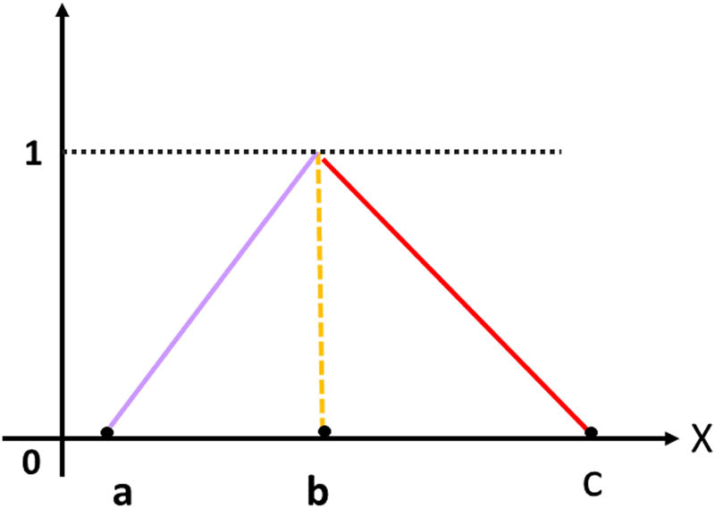
Triangular fuzzy number.

2.2 Expected value of a TFN

Liu and Liu [37] proposed the concept of expected value for a fuzzy number. It is represented by E [ Θ ] and defined as

E [ Θ ] = ∫ 0 + ∞ Cr { Θ ≥ r } d r − ∫ − ∞ 0 Cr { Θ ≥ r } d r ,

where C r is the credibility measure and can be defined for any real number r as follows:

C r { Θ ≥ r } = 1 2 [ Sup t ≤ r μ ( t ) + 1 − Sup t > r μ ( t ) ] ∈ [ 0 , 1 ] ,

Now, the expected value of a triangular fuzzy number is given by [38]

(2.2) E [ A ] = ∫ 0 + ∞ Cr { A ≥ r } d r − ∫ − ∞ 0 Cr { A ≥ r } d r = a + 2 b + c 4 .

2.3 Fuzzy BRN R 0 f

The fuzzy BRN R 0 f is defined as follows [38]:

(2.3) R 0 f = E [ R 0 ( ν ) ] ,

where the expected value of a TFN described in Eq. (2.2) is E [ R 0 ( ν ) ] and the reproduction number is R 0 ( ν ) .

3 TB and HIV/AIDS co-infection model with fuzzy parameters

The total population at any time t , denoted by N ( t ) , is divided into compartments according to their epidemiological status for constructing a co-infection model: susceptible population (S), TB-vaccinated population (V), TB-infected population ( I T ) , recovered population (R), HIV infectious but asymptomatic popuation ( I H ) , population with diagnosed HIV disease without AIDS symptoms ( I A ) , HIV and TB co-infected population ( I H T ) , HIV and TB co-infected population with clinical signs of AIDS ( I A T ) and population at high risk of death due to HIV and TB co-infection ( D H T ) , as proposed by Batu et al. [15].

The proposed model is described by the following system of differential equations:

(3.1) d S d t = ( 1 − ρ ) Λ + ψ R − ( μ + ξ + λ T + λ H − r 1 ) S d V d t = ρ Λ + ξ S − ( μ + σ λ T + λ H ) V d I T d t = λ T S + σ λ T V − ( θ + μ + δ T + λ H ) I T d R d t = θ I T − ( μ + ψ ) R − r 1 S d I H d t = ( S + V ) λ H + α I H T − ( ω + μ + λ T ) I H + r 2 I H T − τ 1 τ 2 I H − ( τ 1 ( 1 − τ 2 ) ) I H d I A d t = ω I H + Φ I A T − ( μ + δ H + κ λ T ) I A + τ 1 τ 2 I H d I H T d t = λ T I H + λ H I T − ( α + ϕ + μ + η 1 ) I H T − r 2 I H T I A T d t = ϕ I H T + κ λ T I A − ( φ + μ + η 2 ) I A T + ( τ 1 ( 1 − τ 2 ) ) I H D H T d t = η 1 I H T + η 2 I A T − ( δ H T + μ ) D H T ,

where λ T = γ T I T + I H T + I A T N − D H T , and λ H = γ H I H + I H T + ε ( I A + I A T ) N − D H T .

The fuzzy model associated with fuzzy parameters can be represented as follows:

(3.2) d S d t = ( 1 − ρ ) Λ + ψ R − ( μ + ξ + λ T + λ H − r 1 ) S d V d t = ρ Λ + ξ S − ( μ + σ λ T + λ H ) V d I T d t = λ T S + σ λ T V − ( θ + μ + δ T ( ν ) + λ H ) I T d R d t = θ ( ν ) I T − ( μ + ψ ) R − r 1 S d I H d t = ( S + V ) λ H + α I H T − ( ω + μ + λ T ) I H + r 2 I H T − τ 1 τ 2 I H − ( τ 1 ( 1 − τ 2 ) ) I H d I A d t = ω I H + Φ I A T − ( μ + δ H ( ν ) + κ λ T ) I A + τ 1 τ 2 I H d I H T d t = λ T I H + λ H I T − ( α + ϕ + μ + η 1 ) I H T − r 2 I H T I A T d t = ϕ I H T + κ λ T I A − ( φ + μ + η 2 ) I A T + ( τ 1 ( 1 − τ 2 ) ) I H D H T d t = η 1 I H T + η 2 I A T − ( δ H T + μ ) D H T ,

where λ T = γ T ( ν ) I T + I H T + I A T N − D H T , and λ H = γ H ( ν ) I H + I H T + ε ( I A + I A T ) N − D H T

The description of the model parameter is given in Table 1.

Table 1

Description of model parameters

Parameter	Description
Λ	Recruitment rate of susceptible population
ρ	Fraction of recruitment to the vaccinated population
1 − σ	Efficacy of vaccination
ξ	Vaccination rate for susceptible individuals
ε , κ	Modification parameters
γ T	Effective transmission rate of TB
γ H	Effective transmission rate of HIV/AIDS
θ	Recovery rate of the TB-infected population
μ	Natural death rate
δ T	Death due to TB disease
ψ	Rate of losing immunity after TB recovery
ω	HIV progression rate for individuals in I H
δ H	HIV induced death rate
η 1 , η 2	Rate at which co-infected individuals risked to death
α	Recovery rate from TB for I H T
φ	Recovery rate from TB for I A T
δ H T	Co-infection-induced death rate
ϕ	HIV progression rate for individuals in I H T
τ 1	Proportion of screening of HIV-infected population selected from I H to I A
τ 2	Proportion of HIV-infected population with no symptoms of AIDS after screening
r 1	Rate at which TB recovered individuals in R move back into the class of susceptible
r 2	Rate at which dually infected individuals in class I H T are treated for TB to move back into class I H

Now, we assume that the effective transmission rate γ T and γ H are fuzzy numbers that depend on the individual virus load. Let γ T = γ T ( ν ) and γ H = γ H ( ν ) be the possibility that virus transmission occurs during an encounter between a susceptible person and an infected person. It was introduced by de Barros et al. [36] and can be described as follows:

(3.3) γ T ( ν ) = 0 , ν < ν min , ν − ν min ν 0 − ν min , ν min ≤ ν ≤ ν 0 , 1 , ν 0 < ν < ν max ,

(3.4) γ H ( ν ) = 0 , ν < ν min , ν − ν min ν 0 − ν min , ν min ≤ ν ≤ ν 0 , 1 , ν 0 < ν < ν max .

γ T ( ν ) and γ H ( ν ) will be highest when the ν is maximum, and negligible when the ν is minimum. ν min represents the minimum virus load needed for disease transmission, while disease transmission is maximum at ν max , which equals 1. The recovery rate θ = θ ( ν ) is also assumed to be a fuzzy number. If the viral load is higher, recovery from infection will take longer. Hence, the fuzzy membership function is taken in the following form:

θ ( ν ) = ( θ 0 − 1 ) ν max ν + 1 , 0 ≤ ν ≤ ν max

where the lowest recovery rate is θ 0 > 0 .

Moreover, as these rates increase as the disease progresses, the death rates δ H for HIV/AIDS and δ T for TB can also be regarded as fuzzy numbers. They can be taken in the following form (Figure 2):

δ H ( ν ) = ( 1 − ζ ) − ε 0 ν min , 0 ≤ ν ≤ ν min , ( 1 − ζ ) , ν min < ν ,

δ T ( ν ) = ( 1 − Γ ) − ε 0 ν min , 0 ≤ ν ≤ ν min , ( 1 − Γ ) , ν min < ν .

Figure 2

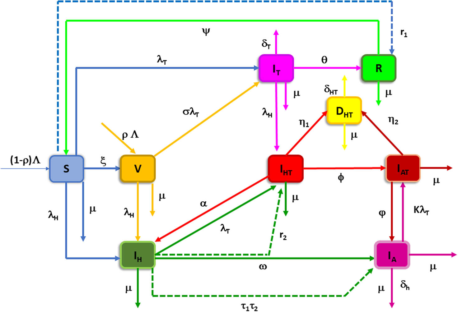
Schematic representation of fuzzy model.

The death rates δ H ( ν ) related to HIV/AIDS and δ T ( ν ) associated with TB show higher values when the viral load ν reaches its peak and the maximum deaths are ( 1 − ζ ) ; ζ ≥ 0 , and ( 1 − Γ ) ; Γ ≥ 0 .

For the purpose to analyze the fuzzy model, we split the model into two sub-models: first the TB sub-model and second the HIV/AIDS sub-model. We discuss these two submodels separately to analyze them in better means.

3.1 Feasibility of the model solution

The feasible region is the positive region R + 9 . Thus, we show that d x i d t ≥ 0 in the region R + 9 . From the model system (3.2), we see that

(3.5) d S d t S = 0 = ( 1 − ρ ) Λ + ψ R ≥ 0 ,

(3.6) d V d t V = 0 = ρ Λ + ξ S ≥ 0 ,

(3.7) d I T d t I T = 0 = λ T S + σ λ T V ≥ 0 ,

(3.8) d R d t R = 0 = θ I T − r 1 S ≥ 0 , ( θ I T ≥ r 1 S ) ,

(3.9) d I H d t I H = 0 = ( S + V ) λ H + α I H T + r 2 I H T ≥ 0 ,

(3.10) d I A d t I A = 0 = ω I H + Φ I A T + τ 1 τ 2 I H ≥ 0 ,

(3.11) d I H T d t I H T = 0 = λ T I H + λ H I T ≥ 0 ,

(3.12) d I A T d t I A T = 0 = ϕ I H T + κ λ T I A + ( τ 1 ( 1 − τ 2 ) ) I H ≥ 0 ,

(3.13) d D H T d t D H T = 0 = η 1 I H T + η 2 I A T ≥ 0 .

Thus, the solution is feasible and positive in the region

Ω = ( S , V , I T , R , I H , I A , I H T , I A T , D H T ) ≥ 0 ∈ R + 9 . Furthermore,

(3.14) d N d t = Λ − μ N − δ T I T + δ H I A − δ H T D H T ,

∴ d N d t ≤ Λ − μ N .

Solving this differential inequalities gives

(3.15) N ( t ) ≤ N ( 0 ) e − μ t + Λ μ ( 1 − e − μ t ) .

As t → ∞ , we have

(3.16) N ( t ) ≤ Λ μ .

Thus, the model solution is bounded and positively invariant in R + 9 .

3.2 Formulation of TB fuzzy sub-model

For this sub-model, I H = 0 , I A = 0 , I H T = 0 , I A T = 0 , and D H T = 0 in (3.2). Therefore, the TB fuzzy sub-model is obtained as follows:

(3.17) d S d t = ( 1 − ρ ) Λ + ψ R − ( Z 1 + λ T ) S d V d t = ρ Λ + ξ S − ( μ + σ λ T ) V d I T d t = λ T S + σ λ T V − Z 2 I T d R d t = θ ( ν ) I T − Z 3 R + r 1 S ,

where Z 1 = ( μ + ξ − r 1 ) , Z 2 = ( θ + μ + δ T ) , Z 3 = ( μ + ψ ) [39].

3.3 TB fuzzy BRN R 0 T f :

Here, we compute the BRN R 0 T for the TB sub-model by using the next-generation matrix method as follows:

d X d t = ℱ ( x ) − V ( x ) , where ℱ = γ T ( ν ) S + σ λ T V 0 and V = Z 2 I T θ I T + Z 3 R − r 1 S .

Then, F ˜ and V ˜ represent the Jacobians of ℱ ( x ) and V ( x ) , respectively, and their expressions can be obtained as follows:

F ˜ = γ T ( ν ) S + σ γ T ( ν ) V 0 0 0 and V ˜ = Z 2 0 − θ Z 3 .

Inserting the disease-free equilibrium (DFE) point E 0 ( 1 − ρ ) Λ Z 3 ( Z 1 Z 3 − ψ r 1 ) , ρ Λ ( Z 1 Z 3 − ψ r 1 ) + ξ ( 1 − ρ ) Λ Z 3 μ ( Z 1 Z 3 − ψ r 1 ) , 0 , r 1 ( 1 − ρ ) Λ ( Z 1 Z 3 − ψ r 1 ) into F V ˜ − 1 we obtain the following result:

(3.18) R 0 T = 1 μ Z 2 γ T ( ν ) ( 1 − ρ ) Λ Z 3 ( Z 1 Z 3 − ψ r 1 ) + γ T σ ( ρ Λ ( Z 1 Z 3 − ψ r 1 ) + ξ ( 1 − ρ ) Λ Z 3 ) Z 2 ( Z 1 Z 3 − ψ r 1 ) .

The analysis of R 0 T , which is dependent on the virus load, can be conducted as follows in three cases:

Case 1. Weak amount of virus load: If ν < ν min , then from Eq. (3.3), we have γ T ( ν ) = 0 , and consequently from (3.18), we have

(3.19) R T ( ν ) = 0 .

Case 2. Medium amount of virus load: If ν min ≤ ν ≤ ν 0 , then from Eq. (3.3), we have γ T ( ν ) = ν − ν min ν 0 − ν min , and consequently from Eq. (3.18), we obtain

(3.20) R T ( ν ) = ν − ν min ν 0 − ν min × μ Z 3 ( 1 − ρ ) Λ + σ ( ρ Λ ( Z 1 Z 3 − ψ r 1 ) ) + ξ ( 1 − ρ ) Λ Z 3 ( μ Z 2 ( Z 1 Z 3 − ψ r 1 ) ) .

Case 3. Strong amount of virus load: If ν 0 < ν < ν max , then from Eq. (3.3), we have γ T ( ν ) = 1 , and consequently from (3.18), we have

(3.21) R T ( ν ) = μ Z 3 ( 1 − ρ ) Λ + σ ( ρ Λ ( Z 1 Z 3 − ψ r 1 ) ) + ξ ( 1 − ρ ) Λ Z 3 ( μ Z 2 ( Z 1 Z 3 − ψ r 1 ) ) .

The BRN R T ( ν ) is a well-defined fuzzy variable that increases with the virus load ν . Consequently, R T ( ν ) ’s expected value is defined precisely and may be expressed in the following manner:

(3.22) R 0 T ( ν ) = 0 , ν − ν min ν 0 − ν min × μ Z 3 ( 1 − ρ ) Λ + σ ( ρ Λ ( Z 1 Z 3 − ψ r 1 ) ) + ξ ( 1 − ρ ) Λ Z 3 ( μ Z 2 ( Z 1 Z 3 − ψ r 1 ) ) , × μ Z 3 ( 1 − ρ ) Λ + σ ( ρ Λ ( Z 1 Z 3 − ψ r 1 ) ) + ξ ( 1 − ρ ) Λ Z 3 ( μ Z 2 ( Z 1 Z 3 − ψ r 1 ) ) .

Now, we obtain the fuzzy reproduction number R 0 T f for TB sub-model as follows by using formulae (2.2) and (2.3):

(3.23) R 0 T f = E [ R 0 T ( ν ) ] ,

or,

(3.24) R 0 T f = μ Z 3 ( 1 − ρ ) Λ + σ ( ρ Λ ( Z 1 Z 3 − ψ r 1 ) ) + ξ ( 1 − ρ ) Λ Z 3 ( μ Z 2 ( Z 1 Z 3 − ψ r 1 ) ) × ( 2 γ T ( ν ) + 1 ) 4 .

3.4 Equilibrium analysis of TB fuzzy sub-model

The following three cases exist while discussing equilibrium analysis of TB fuzzy sub-model:

Case 1. Weak amount of virus load: If ν < ν min , then from Eq. (3.3), we have γ T ( ν ) = 0 . Substituting it into the system (3.17), we obtain

(3.25) E T 0 ( S 0 , V 0 , I T 0 , R 0 ) = Z 3 ( 1 − ρ ) Λ ( Z 1 Z 3 − ψ r 1 ) , ρ Λ ( Z 1 Z 3 − ψ r 1 ) + ξ ( 1 − ρ ) Λ Z 3 μ ( Z 1 Z 3 − ψ r 1 ) , 0 , r 1 ( 1 − ρ ) Λ ( Z 1 Z 3 − ψ r 1 ) ,

which is the DFE point. In this instance, there is no virus present in the entire population. Regarding biology, the disease is eradicated when the population’s viral load decreases below the threshold necessary for disease spread.

Case 2. Medium amount of virus load: If ν 0 < ν ≤ ν max , then from Eq. (3.3), we have γ T ( ν ) = ν − ν min ν 0 − ν min . Substituting it into the system (3.17), we obtain

(3.26) E T * ( S * , V * , I T * , R * ) = Z 3 ( 1 − ρ ) Λ + ψ θ I T * ( Z 3 ( Z 1 + λ T ) − ψ r 1 ) , ρ Λ ( Z 3 ( Z 1 + λ T ) − ψ r 1 ) + ξ ( Z 3 ( 1 − ρ ) Λ + ψ θ I T * ) ( Z 3 ( Z 1 + λ T ) − ψ r 1 ) ( μ + σ λ T ) , I T * , r 1 ( 1 − ρ ) Λ Z 3 + ψ θ I T * + θ I T * ( Z 3 ( Z 3 ( D 1 + λ T ) − ψ r 1 ) ) Z 3 ( Z 3 ( Z 1 + λ T ) − ψ r 1 ) ,

where I T * is given by the quadratic equation

(3.27) K I T * 2 + L I T * + M = 0 ,

where K = σ γ T 2 − γ T 2 ψ θ ,

L = μ Z 3 Z 2 γ T + σ γ T Z 3 Z 2 Z 1 − σ γ T ψ r 1 Z 2 − γ T ξ ψ θ − γ T 2 ( 1 − ρ ) Λ Z 3 σ N − γ T ψ θ μ , M = μ Z 2 ( Z 1 Z 3 − ψ r 1 ) 1 − R 0 N .

Solving (3.27), we obtain

I T * = − L ± L 2 − 4 K M 2 K ,

where M is negative if R 0 > 1 and K < 0 if σ > ψ θ . Then, in this case, I T * has unique positive value. Then, the positive value of I T * is the required value.

Case 3. Strong amount of virus load: If ν 0 < ν ≤ ν min , then from Eq. (3.3), we have γ T ( ν ) = 1 . In this case, we obtain the equilibrium point as follows:

(3.28) E T * * ( S * * , V * * , I T * * , R * * ) = Z 3 ( 1 − ρ ) Λ + ψ θ I T * * ( Z 3 Z 1 N + I T * * − ψ r 1 N ) N , × ρ Λ ( Z 3 Z 1 N + I T * * − ψ r 1 N ) + N ( ξ Z 3 ( 1 − ρ ) Λ + ψ θ I T * * ) ( μ N + σ I T * * ) ( Z 3 Z 1 N + I T * * − ψ r 1 N ) , × I T * * , r 1 ( 1 − ρ ) Λ Z 3 + ψ θ I T * * N + θ I T * * ( Z 3 Z 1 N + I T * * − ψ r 1 N ) Z 3 ( Z 3 Z 1 N + I T * * − ψ r 1 N ) .

In this case, I T * * is obtained by substituting γ T ( ν ) = 1 into Eq. (3.27).

4 Numerical techniques for TB fuzzy sub-model

We find the numerical solution of fuzzy TB sub-model by using the following schemes:

4.1 Forward Euler’s scheme for TB sub-model

The forward Euler’s scheme for the TB sub-model (3.17) can be written as follows:

(4.1) S n + 1 = S n + h ( 1 − ρ ) Λ + ψ R n − S n Z 1 + γ T ( ν ) I T n N ,

(4.2) V n + 1 = V n + h ρ Λ + ξ S n − V n μ + σ γ T ( ν ) I T n N ,

(4.3) I T n + 1 = I T n + h γ T ( ν ) S n + σ V n − D 2 N I T n ,

(4.4) R n + 1 = R n + h [ θ I T n − D 3 R n + r 1 S n ] .

Now, we discuss the following three cases.

Case 1. Weak amount of virus load: If ν < ν min , then from Eq. (3.3), we have γ T ( ν ) = 0 and we have

(4.5) S n + 1 = S n + h [ ( 1 − ρ ) Λ + ψ R n − S n Z 1 ] ,

(4.6) V n + 1 = V n + h [ ρ Λ + ξ S n − V n μ ] ,

(4.7) I T n + 1 = I T n + h σ V n − Z 2 N I T n ,

(4.8) R n + 1 = R n + h [ θ I T n − Z 3 R n + r 1 S n ] .

Case 2. Medium amount of virus load: If ν min ≤ ν ≤ ν 0 , then from Eq. (3.3), we have γ T ( ν ) = ν − ν min ν 0 − ν min . In this case, we obtain

(4.9) S n + 1 = S n + h ( 1 − ρ ) Λ + ψ R n − S n Z 1 + γ T ( ν ) I T n N ,

(4.10) V n + 1 = V n + h ρ Λ + ξ S n − V n μ + σ γ T ( ν ) I T n N ,

(4.11) I T n + 1 = I T n + h γ T ( ν ) S n + σ V n − Z 2 N I T n ,

(4.12) R n + 1 = R n + h [ θ I T n − Z 3 R n + r 1 S n ] .

Case 3. Strong amount of virus load: If ν 0 ≤ ν < ν max , then from Eq. (3.3), we have γ T ( ν ) = 1 . In this case, we have

(4.13) S n + 1 = S n + h ( 1 − ρ ) Λ + ψ R n − S n Z 1 + I T n N ,

(4.14) V n + 1 = V n + h ρ Λ + ξ S n − V n μ + σ I T n N ,

(4.15) I T n + 1 = I T n + h S n + σ V n − Z 2 N I T n ,

(4.16) R n + 1 = R n + h [ θ I T n − Z 3 R n + r 1 S n ] .

4.2 Runge–Kutta method for TB sub-model

The Runge–Kutta method of order 4 is commonly used to solve ordinary differential equations. It is more precise than the Euler’s and other techniques. This method is extensively utilized because it establishes a compromise between simplicity and precision. Here, we give Runge–Kutta method of order 4 for the investigated model as follows:

Step 1:

(4.17) k 1 = h ( 1 − ρ ) Λ + ψ R n − S n Z 1 + γ T ( ν ) I T n N ,

(4.18) l 1 = h ρ Λ + ξ S n − V n μ + σ γ T ( ν ) I T n N ,

(4.19) m 1 = h γ T ( ν ) S n + σ V n − Z 2 N I T n ,

(4.20) n 1 = h [ θ I T n − Z 3 R n + r 1 S n ] ,

Step 2:

(4.21) k 2 = h ( 1 − ρ ) Λ + ψ R n + n 1 2 − S n + k 1 2 × Z 1 + γ T ( ν ) I T n + m 1 2 N ,

(4.22) l 2 = h ρ Λ + ξ S n + k 1 2 − V n + l 1 2 × μ + σ γ T ( ν ) I T n + m 1 2 N ,

(4.23) m 2 = h γ T ( ν ) 1 N I T n + m 1 2 S n + k 1 2 + σ N γ T ( ν ) × I T n + m 1 2 V n + l 1 2 − Z 2 I T n + m 1 2 ,

(4.24) n 2 = h θ I T n + m 1 2 − Z 3 R n + m 1 2 + r 1 S n + k 1 2 .

Step 3:

(4.25) k 3 = h ( 1 − ρ ) Λ + ψ R n + n 2 2 − S n + k 2 2 × Z 1 + γ T ( ν ) I T n + m 2 2 N ,

(4.26) l 3 = h ρ Λ + ξ S n + k 2 2 − V n + l 2 2 × μ + σ γ T ( ν ) I T n + m 2 2 N ,

(4.27) m 3 = h γ T ( ν ) 1 N I T n + m 2 2 S n + k 2 2 + σ N γ T ( ν ) × I T n + m 2 2 V n + l 2 2 − Z 2 I T n + m 2 2 ,

(4.28) n 3 = h θ I T n + m 2 2 − Z 3 R n + n 2 2 + r 1 S n + k 2 2 .

Step 4:

(4.29) k 4 = h [ ( 1 − ρ ) Λ + ψ ( R n + n 3 ) − ( S n + k 3 ) × Z 1 + γ T ( ν ) ( I T n + m 3 ) N ,

(4.30) l 4 = h [ ρ Λ + ξ ( S n + k 3 ) − ( V n + m 3 ) × μ + σ γ T ( ν ) ( I T n + m 3 ) N ,

(4.31) l 4 = h γ T ( ν ) 1 N ( I T n + m 3 ) ( S n + k 3 ) + σ N γ T ( ν ) ( I T n + m 3 ) ( V n + l 2 ) − Z 2 ( I T n + m 3 ) ,

(4.32) n 4 = h [ θ ( I T n + m 3 ) − Z 3 ( R n + n 3 ) + r 1 ( S n + k 3 ) ] .

Final step:

(4.33) S n + 1 = S n + 1 6 [ k 1 + 2 k 2 + 2 k 3 + k 4 ] ,

(4.34) V n + 1 = V n + 1 6 [ l 1 + 2 l 2 + 2 l 3 + l 4 ] ,

(4.35) I T n + 1 = I T n + 1 6 [ m 1 + 2 m 2 + 2 m 3 + m 4 ] ,

(4.36) R n + 1 = R n + 1 6 [ n 1 + 2 n 2 + 2 n 3 + n 4 ] .

4.3 NSFD scheme for TB sub-model

The NSFD scheme combines numerical approaches to solve differential equations using a discrete model. Mickens [9] introduced the NSFD scheme to improve numerical solutions’ precision and stability. The NSFD scheme for the specified model can be expressed specifically as follows:

(4.37) S n + 1 = S n + h { ( 1 − ρ ) Λ + ψ R n } 1 + h Z 1 + γ T ( ν ) I T n N ,

(4.38) V n + 1 = V n + h { ρ Λ + ξ S n } 1 + h μ + σ γ T ( ν ) I T n N ,

(4.39) I T n + 1 = I T n + h { I T S n + σ I T n V n } γ T ( ν ) N 1 + h Z 2 ,

(4.40) R n + 1 = R n + h { θ I T n + r 1 S n } 1 + h Z 2 .

Now, we discuss the following three cases:

Case 1. Weak amount of virus load: If ν < ν min , then from Eq. (3.3), we have γ T ( ν ) = 0 and system given by (4.37)–(4.40) becomes

(4.41) S n + 1 = S n + h { ( 1 − ρ ) Λ + ψ R n } 1 + h Z 1 ,

(4.42) V n + 1 = V n + h { ρ Λ + ξ S n } 1 + h μ ,

(4.43) I T n + 1 = I T n 1 + h Z 2 ,

(4.44) R n + 1 = R n + h { θ I T n + r 1 S n } 1 + h Z 2 .

Case 2. Medium amount of virus load: If ν min ≤ ν ≤ ν 0 , then from Eq. (3.3), we have γ T ( ν ) = ν − ν min ν 0 − ν min . Thus, we obtain

(4.45) S n + 1 = S n + h { ( 1 − ρ ) Λ + ψ R n } 1 + h Z 1 + γ T ( ν ) I T n N ,

(4.46) V n + 1 = V n + h { ρ Λ + ξ S n } 1 + h μ + σ γ T ( ν ) I T n N ,

(4.47) I T n + 1 = I T n + h { I T S n + σ I T n V n } γ T ( ν ) N 1 + h Z 2 ,

(4.48) R n + 1 = R n + h { θ I T n + r 1 S n } 1 + h Z 2 .

Case 3. Strong amount of virus load: If ν 0 < ν < ν max , then from Eq. (3.3), we have γ T ( ν ) = 1 . Thus, we obtain

(4.49) S n + 1 = S n + h { ( 1 − ρ ) Λ + ψ R n } 1 + h Z 1 + I T n N ,

(4.50) V n + 1 = V n + h { ρ Λ + ξ S n } 1 + h μ + σ I T n N ,

(4.51) I T n + 1 = I T n + h { I T S n σ I T n V n } 1 N 1 + h Z 2 ,

(4.52) R n + 1 = R n + h { θ I T n + r 1 S n } 1 + h Z 2 .

4.4 Positivity of the NSFD scheme

If all state variables ( S , V , I T , and R ) in the NSFD scheme are positive at t = 0 , then S n + 1 ≥ 0 , V n + 1 ≥ 0 , I T n + 1 ≥ 0 , and R ‘ n + 1 ≥ 0 .

Proof

Taking into account the state variables ( S , V , I T , and R ) of the NSFD scheme (4.37)–(4.40) and by combining all the equations in the aforementioned system with n = 0 , we arrive at the following expressions:

S 1 = S 0 + h { ( 1 − ρ ) Λ + ψ R 0 } 1 + h Z 1 + γ T ( ν ) I T 0 N ≥ 0 ,

V 1 = V 0 + h { ρ Λ + ξ S 0 } 1 + h μ + σ γ T ( ν ) I T 0 N ≥ 0 ,

I T 1 = I T 0 + h { I T S 0 + σ I T 0 V 0 } γ T ( ν ) N 1 + h Z 2 ≥ 0 ,

R 1 = R 0 + h { θ I T 0 + r 1 S 0 } 1 + h Z 2 ≥ 0 .

By inserting n = 1 , we can advance to the next stage, and then, we have

S 2 = S 1 + h { ( 1 − ρ ) Λ + ψ R 1 } 1 + h Z 1 + γ T ( ν ) I T 1 N ≥ 0 ,

V 2 = V 2 + h { ρ Λ + ξ S 2 } 1 + h μ + σ γ T ( ν ) I T 2 N ≥ 0 ,

I T 2 = I T 2 + h { I T S 2 + σ I T 2 V 2 } γ T ( ν ) N 1 + h Z 2 ≥ 0 ,

R 2 = R 2 + h { θ I T 2 + r 1 S 2 } 1 + h Z 2 ≥ 0 .

Assume next that the aforementioned system of equations guarantees that the variable values have the quality of positivity for n = 2 , 3 , 4 , … , n − 1 , i.e., S n + 1 ≥ 0 , V n + 1 ≥ 0 , I T n + 1 ≥ 0 , R ‘ n + 1 ≥ 0 for n = 1 , 2 , 3 , 4 , … . , n − 1 .

We now analyze the positivity for a random positive integer n ∈ Z , and thus, we find that

S n + 1 = S n + h { ( 1 − ρ ) Λ + ψ R n } 1 + h Z 1 + γ T ( ν ) I T n N ≥ 0 ,

V n + 1 = V n + h { ρ Λ + ξ S n } 1 + h μ + σ γ T ( ν ) I T n N ≥ 0 ,

I T n + 1 = I T n + h { I T S n + σ I T n V n } γ T ( ν ) N 1 + h Z 2 ≥ 0 ,

R n + 1 = R n + h { θ I T n + r 1 S n } 1 + h Z 2 ≥ 0 .

For all positive integer values of n , the suggested strategy, therefore, ensures the positivity of the state variables.□

4.5 Convergence analysis of TB NSFD scheme

Convergence analysis examines whether the numerical solution obtained by a numerical approaches the actual solution of the underlying mathematical model. The behavior of the system’s convergence is largely determined by the eigenvalues of the Jacobian matrix at an equilibrium point. If all of the eigenvalues are strictly less than unity, then the system’s trajectories will eventually converge to the equilibrium point. If any eigenvalue has a magnitude greater than unity, then the corresponding trajectories will deviate from the equilibrium point. When this happens, the system will not be able to achieve equilibrium, and its behavior could turn erratic or chaotic. Now, we will examine the NSFD scheme’s convergence for the aforementioned model. For this purpose, we can express the system (4.37)–(4.40) as follows:

(4.53) U 1 = S + h { ( 1 − ρ ) Λ + ψ R } 1 + h Z 1 + γ T ( ν ) I T N ,

(4.54) W 1 = V + h { ρ Λ + ξ S } 1 + h μ + σ γ T ( ν ) I T N ,

(4.55) X 1 = I T + h { I T S + σ I T V } γ T ( ν ) N 1 + h Z 2 ,

(4.56) Y 1 = R + h { θ I T + r 1 S } 1 + h Z 2 .

Jacobian matrix of the aforementioned system of equations is given by

J = ∂ U ∂ S ∂ U ∂ V ∂ U ∂ I T ∂ U ∂ R ∂ W ∂ S ∂ W ∂ V ∂ W ∂ I T ∂ W ∂ R ∂ X ∂ S ∂ X ∂ V ∂ X ∂ I T ∂ X ∂ R ∂ Y ∂ S ∂ Y ∂ V ∂ Y ∂ I T ∂ Y ∂ R ,

which is discussed in the following in three cases:

Case 1. Weak amount of virus load: If ν < ν min , then from Eq. (3.3), we have γ T ( ν ) = 0 and the aforementioned Jacobian matrix becomes

J ( E T 0 ) = 1 1 + h Z 1 0 0 h ψ 1 + h Z 1 h ξ 1 + h μ 1 1 + h μ 0 0 0 0 0 0 γ 1 h 1 + h Z 2 0 θ h 1 + h Z 2 1 1 + h Z 2 ,

where λ 1 = 0 < 1 , λ 2 = 1 1 + h μ and the third and fourth eigenvalues are given by the following expressions:

(4.57) λ 3 = 2 + h ( Z 1 + Z 2 ) − ( h Z 1 − h Z 2 ) 2 + 4 r 1 h ( 1 + h Z 1 ) ( 1 + h Z 2 ) h ψ 2 ( 1 + h Z 1 ) ( 1 + h Z 2 ) ,

λ 3 < 1 , if the following conditions is satisfied:

(4.58) h 2 [ ( Z 1 − Z 2 ) 2 + 4 r 1 ψ ( 1 + h Z 1 ) ( 1 h Z 2 ) ] < { h ( Z 1 + Z 2 ) + 2 [ 1 − ( 1 + h Z 1 ) ( 1 + h Z 2 ) ] } 2

and

(4.59) λ 4 = 2 + h ( Z 1 + Z 2 ) + ( h Z 1 − h Z 2 ) 2 + 4 r 1 h ( 1 + h Z 1 ) ( 1 + h Z 2 ) h ψ 2 ( 1 + h Z 1 ) ( 1 + h Z 2 )

and λ 4 < 1 if the following conditions is satisfied:

(4.60) h 2 [ ( Z 1 − Z 2 ) 4 r 1 ( 1 + h Z 1 ) ( 1 + h Z 2 ) ] < { 2 h 2 Z 1 Z 2 } 2 .

Case 2. Medium amount of virus load: If ν min ≤ ν ≤ ν 0 , then from Eq. (3.3), we have γ T ( ν ) = ν − ν min ν 0 − ν min and then, we obtain

J ( E T * ) = ∂ U ( E T * ) ∂ S ∂ U ( E T * ) ∂ V ∂ U ( E T * ) ∂ I T ∂ U ( E T * ) ∂ R ∂ W ( E T * ) ∂ S ∂ W ( E T * ) ∂ V ∂ W ( E T * ) ∂ I T ∂ W ( E T * ) ∂ R ∂ X ( E T * ) ∂ S ∂ X ( E T * ) ∂ V ∂ X ( E T * ) ∂ I T ∂ X E T * ∂ R ∂ Y ( E T * ) ∂ S ∂ Y ( E T * ) ∂ V ∂ Y ( E T * ) ∂ I T ∂ Y ( E T * ) ∂ R , ,

where

∂ U ∂ S ( E T * ) = 1 1 + h ( Z 1 + γ T ( ν ) I T N ) , ∂ U ∂ V ( E T * ) = 0 , ∂ U ( E T * ) ∂ R = h ψ 1 + h Z 1 + γ T ( ν ) I T N ,

∂ U ( E T * ) ∂ I T = − h ( 1 − ρ ) Λ + h ψ R + S h γ T ( ν ) N , ∂ W ( E T * ) ∂ S = h ξ 1 + h ( μ + σ γ T ( ν ) I T N ) ,

∂ W ( E T * ) ∂ V = 1 1 + h μ + σ γ T ( ν ) I T N , ∂ W ( E T * ) ∂ I T = − h σ γ T ( ν ) N [ h ρ Λ + h ξ S + V ] ,

∂ W ( E T * ) ∂ R = 0 , ∂ X ( E T * ) ∂ S = h γ T ( ν ) I T 1 + h Z 2 , ∂ X ( E T * ) ∂ I T = [ h γ T ( ν ) [ S + σ V ] + 1 ] N N ( 1 + h Z 2 ) ,

∂ X ( E T * ) ∂ V = h σ γ T ( ν ) I T N ( 1 + h Z 2 ) , ∂ X ( E T * ) ∂ R = 0 , ∂ Y ( E T * ) ∂ S = r 1 h 1 + h Z 2 , ∂ Y ( E T * ) ∂ V = 0 ,

∂ Y ( E T * ) ∂ I T = θ h 1 + h Z 2 , ∂ Y ( E T * ) ∂ R = 1 1 + h Z 2 .

Case 3. Strong amount of virus load: If ν 0 < ν < ν max , then from Eq. (3.3), we have γ T ( ν ) = 1 and then, we obtain

J ( E T * * ) = ∂ U ( E T * * ) ∂ S ∂ U ( E T * * ) ∂ V ∂ U ( E T * * ) ∂ I T ∂ U ( E T * * ) ∂ R ∂ W ( E T * * ) ∂ S ∂ W ( E T * * ) ∂ V ∂ W ( E T * * ) ∂ I T ∂ W ( E T * * ) ∂ R ∂ X ( E T * * ) ∂ S ∂ X ( E T * * ) ∂ V ∂ X ( E T * * ) ∂ I T ∂ X ( E T * * ) ∂ R ∂ Y ( E T * * ) ∂ S ∂ Y ( E T * * ) ∂ V ∂ Y ( E T * * ) ∂ I T ∂ Y ( E T * * ) ∂ R ,

where

∂ U ∂ S ( E T * * ) = 1 1 + h ( Z 1 + I T N ) , ∂ U ∂ V ( E T * * ) = 0 , ∂ U ( E T * * ) ∂ I T = − h ( 1 − ρ ) Λ + h ψ R + S h 1 N ,

∂ U ( E T * * ) ∂ R = h ψ 1 + h Z 1 + I T N , ∂ W ( E T * * ) ∂ S = h ξ 1 + h ( μ + σ I T N ) , ∂ W ( E T * * ) ∂ V = 1 1 + h μ + σ I T N ,

∂ W ( E T * * ) ∂ I T = − h σ 1 N [ h ρ Λ + h ξ S + V ] , ∂ W ( E T * * ) ∂ R = 0 , ∂ X ( E T * * ) ∂ R = 0 , ∂ X ( E T * * ) ∂ S = h I T 1 + h Z 2 ,

∂ X ( E T * * ) ∂ V = h σ I T N ( 1 + h Z 2 ) , ∂ X ( E T * * ) ∂ I T = [ h [ S + σ V ] + 1 ] N N ( 1 + h Z 2 ) , ∂ Y ( E T * * ) ∂ R = 1 1 + h Z 2 , ∂ Y ( E T * * ) ∂ V = 0 ,

∂ Y ( E T * * ) ∂ S = r 1 h 1 + h Z 2 , ∂ Y ( E T * * ) ∂ I T = θ h 1 + h Z 2 .

4.6 Consistency analysis of TB NSFD scheme

Consistency is important in numerical schemes because it connects the discrete equations to the continuous system that they describe. Differential equations derivative operators are discretized using Taylor’s series, and higher-order terms are intentionally eliminated to achieve the necessary accuracy. The removed terms cause a truncation or discretization error in the specified system’s solution. As the mesh size and time steps approach zero, consistency is a key property that guarantees the discretization error will eventually reduce to zero.

Thus, the Taylor series for the susceptible compartment can be written as follows:

(4.61) S n + 1 = S n + h d S d t + h 2 2 ! d 2 S d t 2 + + h 3 3 ! d 3 S d t 2 + … .

From Eq. (4.37), we have

(4.62) S n + 1 1 + h Z 1 + γ T ( ν ) I T n N = S n + h { ( 1 − ρ ) Λ + ψ R n }

S n + h d S d t + h 2 2 ! d 2 S d t 2 + + h 3 3 ! d 3 S d t 2 + … 1 + h Z 1 + γ T ( ν ) I T n N = S n + h { ( 1 − ρ ) Λ + ψ R n }

S n Z 1 + γ T ( ν ) I T n N + d S d t + h d S d t Z 1 + γ T ( ν ) I T n N + … = { ( 1 − ρ ) Λ + ψ R n } .

Taking h → 0 , we obtain

d S d t = ( 1 − ρ ) Λ + ψ R − ( Z 1 + λ T ) S .

Similarly, applying the Taylor series for Eqs. (4.38)–(4.40), we obtain

d V d t = ρ Λ + ξ S − ( μ + σ λ T ) V , d I T d t = λ T S + σ λ T V − Z 2 I T , d R d t = θ ( ν ) I T − Z 3 R + r 1 S .

5 Formulation of HIV/AIDS fuzzy sub-model

For this sub-model, I T = 0 , I H T = 0 , D H T = 0 , and I A T = 0 in (3.2). Therefore, the HIV/AIDS sub-model is obtained as follows:

(5.1) d S d t = ( 1 − ρ ) Λ + ψ R − ( Z 1 + λ H ) S d V d t = ρ Λ + ξ S − ( μ + λ H ) V d I H d t = ( S + V ) λ H − ( Z 4 + τ 1 τ 2 + ( τ 1 ( 1 − τ 2 ) ) ) I H d I A d t = ω I H − Z 5 I A + τ 1 τ 2 I H ,

where λ H = γ H ( ν ) I H + ε I A N , Z 4 = ( ω + μ ) , Z 5 = ( μ + δ H ) .

5.1 HIV/AIDS fuzzy BRN R 0 H f

Here, we compute the BRN R 0 H for the HIV/AIDS sub-model by using the next-generation matrix method as follows:

Let d X d t = ℱ ( x ) − V ( x ) , where ℱ = ( S + V ) λ H 0 and V = ( Z 4 + τ 1 ) I H Z 5 I A − τ 1 τ 2 I H − ω I H . Now, F and V represent the Jacobians of ℱ ( x ) and V ( x ) , respectively, and their expressions can be obtained as follows:

F = γ H ε γ H 0 0 and V = ( Z 4 + τ 1 ) 0 − ( τ 1 τ 2 + ω ) Z 5 .

The following result is obtained by substituting the DFE point E 0 into F V − 1 ,

(5.2) R 0 = γ H ( Z 4 + τ 1 ) ( 1 + ε ( ω + τ 1 τ 2 ) Z 5 ) .

Here, we compute the BRN R 0 H for the HIV/AIDS sub-model by using the next-generation matrix method as follows:

Case 1. Weak amount of virus load: If ν < ν min , then from Eq. (3.4), we have γ H ( ν ) = 0 , and consequently from (5.1), we have

(5.3) R H ( ν ) = 0 .

Case 2. Medium amount of virus load: If ν min ≤ ν ≤ ν 0 , then from Eq. (3.4), we have γ H ( ν ) = ν − ν min ν 0 − ν min , and consequently from Eq. (5.1), we obtain

(5.4) R H ( ν ) = ν − ν min ν Max − ν min Z 5 + ε ( ω + τ 1 τ 2 ) Z 5 ( Z 4 + τ 1 ) .

Case 3. Strong amount of virus load: If ν 0 < ν < ν max , then from Eq. (3.4), we have γ H ( ν ) = 1 , and consequently from (5.1), we have

(5.5) R H ( ν ) = Z 5 + ε ( ω + τ 1 τ 2 ) Z 5 ( Z 4 + τ 1 ) .

As a well-defined fuzzy variable, the BRN R 0 H ( ν ) increases with the viral load ν . Consequently, we have a well-defined expected value for R 0 H ( ν ) , which can be expressed as follows:

(5.6) R 0 H ( ν ) = 0 , ν − ν min ν Max − ν min × Z 5 + ε ( ω + τ 1 τ 2 ) Z 5 ( Z 4 + τ 1 ) , × Z 5 + ε ( ω + τ 1 τ 2 ) Z 5 ( Z 4 + τ 1 ) .

Now, we obtain the fuzzy reproduction number R 0 H for HIV/AIDS sub-model as follows by using formulae (2.2) and (2.3):

(5.7) R 0 H f = E [ R 0 H ( ν ) ]

(5.8) R 0 H f = Z 5 + ε ( ω + τ 1 τ 2 ) Z 5 ( Z 4 + τ 1 ) ( 2 γ T ( ν ) + 1 ) 4 .

5.2 Equilibrium analysis of HIV/AIDS fuzzy sub-model

The following three cases exist while discussing equilibrium analysis of HIV/AIDS model fuzzy sub-model.

Case 1. Weak amount of virus load: If ν < ν min , then, from Eq. (3.4), we have γ H ( ν ) = 0 . Substituting it into system (5.1), we obtain

(5.9) E T 0 ( S 0 , V 0 , I H 0 , I A 0 ) = ( 1 − ρ ) Λ ( Z 1 ) , ρ Λ Z 1 + ξ ( 1 − ρ ) Λ μ Z 1 , 0 , 0 ,

which is the DFE point. In this instance, there is no virus present in the entire population. Regarding biology, the disease is eradicated when the population’s viral load falls below the threshold value necessary for disease spread.

Case 2. Medium amount of virus load: If ν min ≤ ν ≤ ν 0 , then from Eq. (3.4), we have γ T ( ν ) = ν − ν min ν 0 − ν min . Substituting it into system (5.1), we obtain

(5.10) E H * = [ S * , V * , I H * , I A * , ] ,

S * = ( 1 − ρ ) Λ ( Z 1 + λ H ) , V * = ρ Λ ( Z 1 + λ H ) + ξ ( 1 − ρ ) Λ ( μ + λ H ) ( Z 1 + λ H ) , I A * = ( τ 1 τ 2 + ω ) I H Z 5 ,

where I H * is given by the quadratic equation

(5.11) K I H * 2 + L I H * + M = 0 ,

where

K = Z 5 + ε ( ω + τ 1 τ 2 ) Z 5 ( Z 4 + τ 1 ) 2 γ H 2 ( Z 4 + τ 1 ) , L = Z 5 + ε ( ω + τ 1 τ 2 ) Z 5 ( Z 4 + τ 1 ) 2 γ H 2 ( Z 4 + ( Z 1 + μ ) + Λ ) ,

and

M = Z 1 μ ( Z 4 + τ 1 ) 1 − R 0 Z 1 μ N [ ( 1 − ρ ) Λ μ + ρ Λ Z 1 + ξ ( 1 − ρ ) Λ ] ,

I H * = − L ± L 2 − 4 K M 2 K ,

where M is negative, if R 0 > 1 and K > 0 , then I H * has unique positive value. The positive value of I H * is the required value.

Case 3. Strong amount of virus load: If ν 0 < ν < ν max , then from Eq. (3.4), we have γ H ( ν ) = 1 . Consequently, we obtain

(5.12) E H * * = [ S * * , V * * , I H * * , I A * * ] ,

S * = ( 1 − ρ ) Λ ( Z 1 + λ H ) , V * = ρ Λ ( Z 1 + λ H ) + ξ ( 1 − ρ ) Λ ( μ + λ H ) ( Z 1 + λ H ) , I A * = ( τ 1 τ 2 + ω ) I H Z 5 .

Substituting γ H ( ν ) = 1 into Eq. (5.12) yields I H * * . Here, endemic equilibrium points are E * and E * * . When the virus surpasses the minimal threshold and persists in infecting the population, these points arise.

6 Numerical techniques for HIV/AIDS fuzzy sub-model

We find the numerical solution of fuzzy HIV/AIDS sub-model by using the following schemes:

6.1 Forward Euler’s scheme for HIV/AIDS sub-model

The forward Euler’s scheme for HIV/AIDS sub-model (5.1) can be expressed as follows:

(6.1) S n + 1 = S n + h ( 1 − ρ ) Λ − S n Z 1 + γ H ( ν ) I H n + ε I A n N ,

(6.2) V n + 1 = V n + h ρ Λ + ξ S n − V n μ + γ H ( ν ) I H n + ε I A n N ,

(6.3) I H n + 1 = I H n + h γ H ( ν ) I H n + ε I A n N S n + γ H ( ν ) I H n + ε I A n N V n × { Z 4 + τ 1 τ 2 + ( τ 1 ( 1 − τ 2 ) ) } I H n ,

(6.4) I A n + 1 = I A n + h [ ω I H n − Z 5 I A n + τ 1 τ 2 I H n ] .

Now, we discuss the following three cases:

Case 1. Weak amount of virus load: If ν < ν min , then from Eq. (3.4), we have γ H ( ν ) = 0 and then, we obtain

(6.5) S n + 1 = S n + h [ ( 1 − ρ ) Λ − S n Z 1 ] ,

(6.6) V n + 1 = V n + h [ ρ Λ + ξ S n − V n μ ] ,

(6.7) I H n + 1 = I H n + h [ − { Z 4 + τ 1 } I H n ] ,

(6.8) I A n + 1 = I A n + h [ ω I H n − Z 5 I A n + τ 1 τ 2 I H n ] .

Case 2. Medium amount of virus load: If ν min ≤ ν ≤ ν 0 , then from Eq. (3.4), we have γ H ( ν ) = ν − ν min ν 0 − ν min and then, we obtain

(6.9) S n + 1 = S n + h ( 1 − ρ ) Λ − S n Z 1 + γ H ( ν ) I H n + ε I A n N ,

(6.10) V n + 1 = V n + h ρ Λ + ξ S n − V n μ + γ H ( ν ) I H n + ε I A n N ,

(6.11) I H n + 1 = I H n + h γ H ( ν ) I H n + ε I A n N S n + γ H ( ν ) I H n + ε I A n N V n { Z 4 + τ 1 τ 2 + ( τ 1 ( 1 − τ 2 ) ) } I H n ,

(6.12) I A n + 1 = I A n + h [ ω I H n − Z 5 I A n + τ 1 τ 2 I H n ] .

Case 3. Strong amount of virus load: If ν 0 < ν < ν max , then from Eq. (3.4), we have γ H ( ν ) = 1 and then, we obtain

(6.13) S n + 1 = S n + h ( 1 − ρ ) Λ − S n Z 1 + I H n + ε I A n N ,

(6.14) V n + 1 = V n + h ρ Λ + ξ S n − V n μ + I H n + ε I A n N ,

(6.15) I H n + 1 = I H n + h I H n + ε I A n N S n + I H n + ε I A n N V n × { Z 4 + τ 1 τ 2 + ( τ 1 ( 1 − τ 2 ) ) } I H n ,

(6.16) I A n + 1 = I A n + h [ ω I H n − Z 5 I A n + τ 1 τ 2 I H n ] .

6.2 Runge–Kutta method of order 4 for HIV/AIDS sub-model

Here, we give Runge–Kutta method of order 4 for the investigated HIV/AIDS sub-model as follows:

Step 1:

(6.17) k 1 = h ( 1 − ρ ) Λ − S n Z 1 + γ H ( ν ) I H n + ε I A n N ,

(6.18) l 1 = h ρ Λ + ξ S n − V n μ + γ H ( ν ) I H n + ε I A n N ,

(6.19) m 1 = h γ H ( ν ) I H n + ε I A n N ( S n + V n ) N − ( Z 4 + τ 1 τ 2 + ( τ 1 ( 1 − τ 2 ) ) ) I H n ,

(6.20) n 1 = h [ ω I H n − Z 5 I A n + τ 1 τ 2 I H n ] .

Step 2:

(6.21) k 2 = h ( 1 − ρ ) Λ − S n + k 1 2 Z 1 + γ H ( ν ) I H n + m 1 2 N + ε I A n + n 1 2 N ,

(6.22) l 2 = h ρ Λ + ξ S n + k 1 2 − V n + l 1 2 μ + γ H ( ν ) I H n + m 1 2 N + ε I A n + n 1 2 N ,

(6.23) m 2 = h γ H ( ν ) N I H n + m 1 2 + ε I A n + n 1 2 S n + k 1 2 + V n + l 1 2 − ( Z 4 + τ 1 ) I H n + m 1 2 ,

(6.24) n 2 = h ω I H n + m 1 2 − Z 5 I A n + n 1 2 + τ 1 τ 2 I H n + m 1 2 .

Step 3:

(6.25) k 3 = h ( 1 − ρ ) Λ − S n + k 2 2 Z 1 + γ H ( ν ) I H n + m 2 2 N + ε I A n + n 2 2 N ,

(6.26) l 3 = h ρ Λ + ξ S n + k 2 2 − V n + l 2 2 μ + γ H ( ν ) I H n + m 2 2 N + ε I A n + n 2 2 N ,

(6.27) m 3 = h γ H ( ν ) N I H n + m 2 2 + ε I A n + n 2 2 S n + k 2 2 + V n + l 2 2 − ( Z 4 + τ 1 ) I H n + m 2 2 ,

(6.28) n 3 = h ω I H n + m 2 2 − Z 5 I A n + n 2 2 + τ 1 τ 2 I H n + m 2 2 .

Step 4:

(6.29) k 4 = h ( 1 − ρ ) Λ − ( S n + k 3 ) Z 1 + γ H ( ν ) N ( I H n + m 3 ) + ε ( I A n + n 3 ) ,

(6.30) l 4 = h ρ Λ + ξ ( S n + k 3 ) − ( V n + l 3 ) μ + γ H ( ν ) N { ( I H n + m 3 ) + ε ( I A n + n 3 ) } ,

(6.31) m 4 = h γ H ( ν ) N { ( I H n + m 3 ) + ε ( I A n + l 3 ) } { ( s n + k 3 ) + ( V n + l 3 ) − ( Z 4 + τ 1 ) } ( I H n + m 3 ) ,

(6.32) n 4 = h [ ω ( I H n + m 3 ) − Z 5 ( I A n + n 3 ) + τ 1 τ 2 ( I H n + m 3 ) ] .

Final step:

(6.33) S n + 1 = S n + 1 6 [ k 1 + 2 k 2 + 2 k 3 + k 4 ] ,

(6.34) V n + 1 = V n + 1 6 [ l 1 + 2 l 2 + 2 l 3 + l 4 ] ,

(6.35) I H n + 1 = I T n + 1 6 [ m 1 + 2 m 2 + 2 m 3 + m 4 ] ,

(6.36) I A n + 1 = I A n + 1 6 [ n 1 + 2 n 2 + 2 n 3 + n 4 ] .

6.3 NSFD scheme for HIV/AIDS sub-model

The NSFD scheme for the given HIV/AIDS model can be expressed as follows:

(6.37) S n + 1 = S n + h { ( 1 − ρ ) Λ } 1 + h Z 1 + γ H ( ν ) I H n + ε I A n N ,

(6.38) V n + 1 = V n + h { ρ Λ + ξ S n } 1 + h μ + γ H ( ν ) I H n + ε I A n N ,

(6.39) I H n + 1 = h γ H ( ν ) ε I A n V n + N I H n 1 + h ( γ H ( ν ) S n − N Z 4 ) ,

(6.40) I A n + 1 = h { ω I H n + τ 1 τ 2 I H n } + I A n 1 + h Z 5 .

Now, we discuss the following three cases:

Case 1. Weak amount of virus load: If ν < ν min , then from Eq. (3.4), we have γ H ( ν ) = 0 and system given by (6.37)–(6.40) becomes

(6.41) S n + 1 = S n + h { ( 1 − ρ ) Λ } 1 + h Z 1 ,

(6.42) V n + 1 = V n + h { ρ Λ + ξ S n } 1 + h μ ,

(6.43) I H n + 1 = N I H n 1 + h N ( z 4 − τ 1 ) ,

(6.44) I A n + 1 = h { ω I H n + τ 1 τ 2 I H n } + I A n 1 + h z 5 .

Case 2. Medium amount of virus load: If ν min ≤ ν ≤ ν 0 , then from Eq. (3.4), we have γ H ( ν ) = ν − ν min ν 0 − ν min , we obtain

(6.45) S n + 1 = S n + h { ( 1 − ρ ) Λ } 1 + h Z 1 + γ H ( ν ) I H n + ε I A n N ,

(6.46) V n + 1 = V n + h { ρ Λ + ξ S n } 1 + h μ + γ H ( ν ) I H n + ε I A n N ,

(6.47) I H n + 1 = h γ H ( ν ) ε I A n V n + N I H n 1 + h ( γ H ( ν ) S n − N Z 4 ) ,

(6.48) I A n + 1 = h { ω I H n + τ 1 τ 2 I H n } + I A n 1 + h Z 5 .

Case 3. Strong amount of virus load: If ν 0 < ν < ν max , then from Eq. (3.4), we have γ H ( ν ) = 1 , and we have

(6.49) S n + 1 = S n + h { ( 1 − ρ ) Λ } 1 + h Z 1 + I H n + ε I A n N ,

(6.50) V n + 1 = V n + h { ρ Λ + ξ S n } 1 + h μ + I H n + ε I A n N ,

(6.51) I H n + 1 = h ε I A n V n + N I H n 1 + h ( S n − N Z 4 ) ,

(6.52) I A n + 1 = h { ω I H n + τ 1 τ 2 I H n } + I A n 1 + h Z 5 .

6.4 Positivity of the NSFD scheme

Theorem 1

If all the state variables ( S , V , I H , and I A ) in the NSFD scheme are positive at t = 0 , then S n + 1 ≥ 0 , V n + 1 ≥ 0 , I H n + 1 ≥ 0 , and I A n + 1 ≥ 0 .

Proof

Taking into account the state variables ( S , V , I H , and I A ) of the NSFD scheme (6.37)–(6.40) and by combining all the equations in the aforementioned system with n = 0 , we arrive at the following expressions:

S 1 = S 0 + h { ( 1 − ρ ) Λ } 1 + h Z 1 + γ H ( ν ) I H 0 + ε I A 0 N ≥ 0 ,

V 1 = V 0 + h { ρ Λ + ξ S 0 } 1 + h μ + γ H ( ν ) I H 0 + ε I A 0 N ≥ 0 ,

I H 1 = h γ H ( ν ) ε I A 0 V 0 + N I H 0 1 + h ( γ H ( ν ) S 0 − N Z 4 ) ≥ 0 ,

I A 1 = h { ω I H 0 + τ 1 τ 2 I H 0 } + I A 0 1 + h Z 5 ≥ 0 .

By inserting n = 1 , we can advance to the next stage, and then, we have

S 2 = S 1 + h { ( 1 − ρ ) Λ } 1 + h Z 1 + γ H ( ν ) I H 1 + ε I A 1 N ≥ 0 ,

V 2 = V 1 + h { ρ Λ + ξ S 1 } 1 + h μ + γ H ( ν ) I H 1 + ε I A 1 N ≥ 0 ,

I H 2 = h γ H ( ν ) ε I A 1 V 1 + N I H 1 1 + h ( γ H ( ν ) S 1 − N Z 4 ) ≥ 0 .

I A 2 = h { ω I H 1 + τ 1 τ 2 I H 1 } + I A 1 1 + h Z 5 ≥ 0 .

Assume next that the aforementioned system of equations guarantees that the variable values have the quality of positivity for n = 2 , 3 , 4 , … , n − 1 , i.e., S n + 1 ≥ 0 , V n + 1 ≥ 0 , I H n + 1 ≥ 0 , I A ‘ n + 1 ≥ 0 for n = 1 , 2 , 3 , 4 , … , n − 1 .

We now analyze the positivity for a random positive integer n ∈ Z , and thus, we find that

S n + 1 = S n + h { ( 1 − ρ ) Λ } 1 + h Z 1 + γ H ( ν ) I H n + ε I A n N ≥ 0 ,

V n + 1 = V n + h { ρ Λ + ξ S n } 1 + h μ + γ H ( ν ) I H n + ε I A n N ≥ 0 ,

I H n + 1 = h γ H ( ν ) ε I A n V n + N I H n 1 + h ( γ H ( ν ) S n − N Z 4 ) ≥ 0 ,

I A n + 1 = h { ω I H n + τ 1 τ 2 I H n } + I A n 1 + h Z 5 ≥ 0 .

For all positive integer values of n , the suggested strategy, therefore, ensures the positivity of the state variables.□

6.5 Convergence analysis of the NSFD scheme of HIV/AIDS

Now, we will examine the NSFD scheme’s convergence for the aforementioned model. For this purpose, we can express system (6.37)–(6.40) as follows:

(6.53) U 1 = S + h { ( 1 − ρ ) Λ } 1 + h Z 1 + γ H ( ν ) I H + ε I A N ,

(6.54) W 1 = V + h { ρ Λ + ξ S } 1 + h μ + γ H ( ν ) I H + ε I A N ,

(6.55) X 1 = h γ H ( ν ) ε I A V + N I H 1 + h ( γ H ( ν ) S − N Z 4 ) ,

(6.56) Y 1 = h { ω I H + τ 1 τ 2 I H } + I A 1 + h Z 5 .

Jacobian matrix of the aforementioned system of equations is given by

J = ∂ U 1 ∂ S ∂ U 1 ∂ V ∂ U 1 ∂ I H ∂ U 1 ∂ I A ∂ W 1 ∂ S ∂ W 1 ∂ V ∂ W 1 ∂ I H ∂ W 1 ∂ I A ∂ X 1 ∂ S ∂ X 1 ∂ V ∂ X 1 ∂ I H ∂ X 1 ∂ I A ∂ Y 1 ∂ S ∂ Y 1 ∂ V ∂ Y 1 ∂ I H ∂ Y 1 ∂ I A ,

which is discussed in the following in three cases:

Case 1. Weak amount of virus load: If ν < ν min , from Eq. (3.4), we have γ H ( ν ) = 0 and the aforementioned Jacobian matrix becomes

J ( E H 0 ) = 1 1 + h Z 1 0 0 0 h ξ 1 + h μ 1 1 + h μ 0 0 0 0 a 33 − λ a 34 0 0 a 43 a 44 − λ ,

where λ 1 = 1 1 + h Z 1 < 1 , λ 2 = h ξ 1 + h D Z 1 and the third and fourth eigenvalues are given by the following expressions:

(6.57) λ 3 = 1 2 + ( a 33 + a 44 ) − a 33 2 + 4 a 34 a 43 − 2 a 33 a 44 + a 44 2 ,

λ 3 < 1 , if the following condition is satisfied:

(6.58) ( a 33 + a 44 ) < 2 − a 33 2 + 4 a 34 a 43 − 2 a 33 a 44 + a 44 2

and

(6.59) λ 4 = 1 2 + ( a 33 + a 44 ) − a 33 2 + 4 a 34 a 43 − 2 a 33 a 44 + a 44 2

and λ 4 < 1 , if the following condition is satisfied:

(6.60) ( a 33 + a 44 ) < 2 + a 33 2 + 4 a 34 a 43 − 2 a 33 a 44 + a 44 2 ,

where a 33 = N [ 1 + h { γ H ( ν ) − N Z 4 − N τ 1 } ] , a 34 = ε V 1 + h { γ H ( ν ) − N Z 4 − N τ 1 } , a 43 = h ( ω + τ 1 τ 2 ) 1 + h Z 5 , and a 44 = 1 1 + h Z 5 .

Case 2. Medium amount of virus load: If ν min ≤ ν ≤ ν 0 , then from Eq. (3.4), we have γ H ( ν ) = ν − ν min ν 0 − ν min , and we obtain

J ( E H * ) = ∂ U ( E H * ) ∂ S ∂ U ( E H * ) ∂ V ∂ U ( E H * ) ∂ I H ∂ U ( E H * ) ∂ I A ∂ W ( E H * ) ∂ S ∂ W ( E H * ) ∂ V ∂ W ( E H * ) ∂ I T ∂ W ( E H * ) ∂ I A ∂ X ( E H * ) ∂ S ∂ X ( E H * ) ∂ V ∂ X ( E H * ) ∂ I T ∂ X E H * ∂ I A ∂ Y ( E H * ) ∂ S ∂ Y ( E H * ) ∂ V ∂ Y ( E H * ) ∂ I T ∂ Y ( E H * ) ∂ I A ,

where

∂ U 1 ∂ S ( E H * ) = 1 1 + h ( Z 1 + γ H ( ν ) N ) { I H + ε I A } , ∂ U 1 ∂ V ( E T * ) = 0 ,

∂ U 1 ( E H * ) ∂ I H = − ( h ( 1 − ρ ) Λ + S ) γ H ( ν ) N 1 + h Z 1 + γ H ( ν ) N I H + ε I A 2 , ∂ U 1 ( E H * ) ∂ I A = − ( h ( 1 − ρ ) Λ + S ) γ H ( ν ) ε N 1 + h Z 1 + γ H ( ν ) N I H + ε I A 2 ,

∂ W 1 ( E H * ) ∂ S = h ξ 1 + h ( μ + γ H ( ν ) N { I H + ε I A } ) , ∂ W 1 ( E H * ) ∂ V = 1 1 + h ( μ + γ H ( ν ) N { I H + ε I A } ) ,

∂ W 1 ( E H * ) ∂ I H = − h ( ρ Λ + ξ S ) + V γ H ( ν ) N 1 + h ( μ + γ H ( ν ) N { I H + ε I A } ) 2 , ∂ W 1 ( E H * ) ∂ I A = − h ( ρ Λ + ξ S ) + V γ H ( ν ) ε N 1 + h ( μ + γ H ( ν ) N { I H + ε I A } ) 2 ,

∂ X 1 ( E T * ) ∂ S = { h γ H ( ν ) ε I A V + N I H } ( h γ H ( ν ) ) [ 1 + h { γ H ( ν ) S − N Z 4 − N τ 1 } ] 2 , ∂ X 1 ( E T * ) ∂ V = ε I A [ 1 + h { γ H ( ν ) S − N Z 4 − N τ 1 } ] ,

∂ X 1 ( E T * ) ∂ I H = N [ 1 + h { γ H ( ν ) S − N Z 4 − N τ 1 } ] , ∂ X ( E T * ) ∂ I A = ε V [ 1 + h { γ H ( ν ) S − N Z 4 − N τ 1 } ] ,

∂ Y 1 ( E T * ) ∂ S = 0 , ∂ Y 1 ( E T * ) ∂ V = 0 , ∂ Y ( E T * ) ∂ I T = 1 1 + h Z 5 , ∂ Y ( E T * ) ∂ R = h ( ω + τ 1 τ 2 ) 1 + h Z 5 .

Case 3. Strong amount of virus load: If ν 0 < ν < ν max , then from Eq. (3.4), we have γ H ( ν ) = 1 ,

J ( E H * ) = ∂ U 1 ( E H * * ) ∂ S ∂ U 1 ( E H * * ) ∂ V ∂ U 1 ( E H * * ) ∂ I H ∂ U 1 ( E H * * ) ∂ I A ∂ W 1 ( E H * * ) ∂ S ∂ W 1 ( E H * * ) ∂ V ∂ W 1 ( E H * * ) ∂ I T ∂ W 1 ( E H * * ) ∂ I A ∂ X 1 ( E H * * ) ∂ S ∂ X 1 ( E H * * ) ∂ V ∂ X 1 ( E H * * ) ∂ I T ∂ X 1 E H * * ∂ I A ∂ Y 1 ( E H * * ) ∂ S ∂ Y 1 ( E H * * ) ∂ V ∂ Y 1 ( E H * * ) ∂ I T ∂ Y 1 ( E H * * ) ∂ I A ,

where

∂ U 1 ∂ S ( E H * * ) = 1 1 + h ( Z 1 + 1 N ) { I H + ε I A } , ∂ U 1 ∂ V ( E T * * ) = 0 ,

∂ U 1 ( E H * * ) ∂ I H = − ( h ( 1 − ρ ) Λ + S ) 1 N 1 + h Z 1 + 1 N I H + ε I A 2 , ∂ U 1 ( E H * * ) ∂ I A = − ( h ( 1 − ρ ) Λ + S ) ε N 1 + h Z 1 + 1 N I H + ε I A 2 ,

∂ W 1 ( E H * * ) ∂ S = h ξ 1 + h ( μ + 1 N { I H + ε I A } ) , ∂ W 1 ( E H * * ) ∂ V = 1 1 + h ( μ + 1 N { I H + ε I A } ) ,

∂ W 1 ( E H * * ) ∂ I H = − h ( ρ Λ + ξ S ) + V 1 N 1 + h ( μ + 1 N { I H + ε I A } ) 2 , ∂ W 1 ( E H * * ) ∂ I A = − h ( ρ Λ + ξ S ) + V ε N 1 + h ( μ + 1 N { I H + ε I A } ) 2 ,

∂ X 1 ( E T * * ) ∂ S = { h ε I A V + N I H } ( h ) [ 1 + h { S − N Z 4 − N τ 1 } ] 2 , ∂ X 1 ( E T * * ) ∂ V = ε I A [ 1 + h { S − N Z 4 − N τ 1 } ] ,

∂ X 1 ( E T * * ) ∂ I H = N [ 1 + h { S − N Z 4 − N τ 1 } ] , ∂ X 1 ( E T * * ) ∂ I A = ε V [ 1 + h { S − N Z 4 − N τ 1 } ] , ∂ Y 1 ( E T * * ) ∂ S = 0 ,

∂ Y 1 ( E T * * ) ∂ V = 0 , ∂ Y 1 ( E T * * ) ∂ I T = 1 1 + h Z 5 , ∂ Y 1 ( E T * * ) ∂ R = h ( ω + τ 1 τ 2 ) 1 + h Z 5 .

6.6 Consistency analysis of HIV/AIDS fuzzy sub-model

Thus, the Taylor series for susceptible compartment can be written as follows:

(6.61) S n + 1 = S n + h d S d t + h 2 2 ! d 2 S d t 2 + + h 3 3 ! d 3 S d t 2 + …

From Eq. (6.37), we have

(6.62) S n + 1 1 + h Z 1 + γ H ( ν ) { I H + ε I A } N = S n + h ( 1 − ρ ) Λ ,

S n + h d S d t + h 2 2 ! d 2 S d t 2 + + h 3 3 ! d 3 S d t 2 + … 1 + h Z 1 + γ H ( ν ) { I H + ε I A } N = S n + h ( 1 − ρ ) Λ ,

S n Z 1 + γ H ( ν ) { I H + ε I A } N + d S d t + h d S d t Z 1 + γ H ( ν ) { I H + ε I A } N + … = ( 1 − ρ ) Λ .

Taking h → 0, we obtain

d S d t = ( 1 − ρ ) Λ − ( Z 1 + λ H ) S .

Similarly, applying the Taylor series for Eqs (6.38)–(6.40), we obtain

d V d t = ρ Λ + ξ S − ( μ + σ λ T ) V d I H d t = ( S + V ) λ H − ( Z 4 + τ 1 τ 2 + ( τ 1 ( 1 − τ 2 ) ) ) I H d I A d t = ω I H − Z 5 I A + τ 1 τ 2 I H .

Table 2 contains detailed information on the model parameters.

Table 2

Values and sources of model parameters

Parameter	Value	Source
Λ	200	Fitted
ρ	0.99	Fitted
1 − σ	0.99	Estimated
ξ	0.935	Fitted
ε , κ	0.0998, 0.0224	Fitted
γ T	0.009768	Fitted
γ H	0.00798	Fitted
θ	0.21	Estimated
μ	0.009	Fitted
δ T	0.009	Fitted
ψ	0.89	Estimated
ω	0.011	Fitted
δ H	7.99	Fitted
τ 1	0.0001	Fitted
τ 2	0.009	Fitted
r 1	0.9	Fitted

7 Numerical simulation

Numerical simulations validate the findings of the co-infection model of TB and HIV/AIDS with fuzzy parameters. The effects of factors on the spread and control co-infection of TB and HIV/AIDS are evaluated. Parameter values from Table 2 are used to perform simulations using MATLAB software. Various types of plots are shown and explained in the following [40].

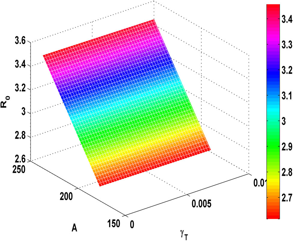
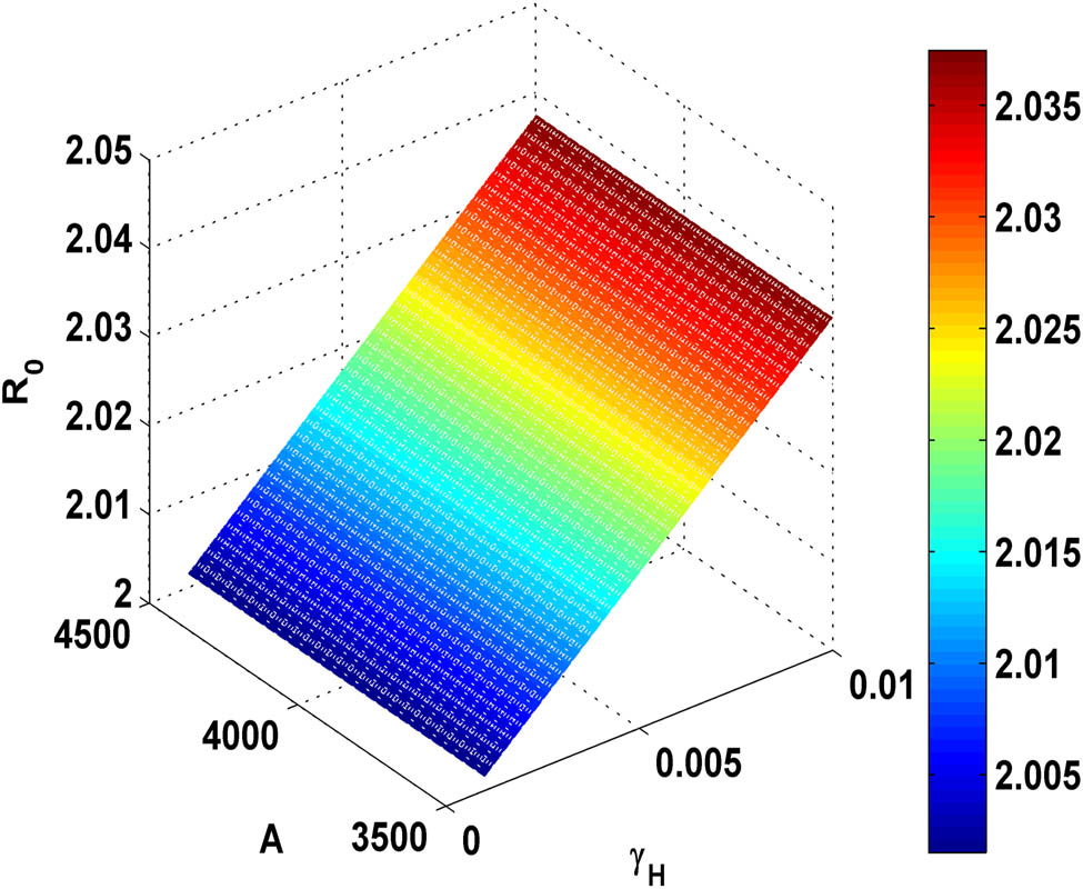
Figure 3 demonstrates that as the value of γ T and σ increases, the value of fuzzy reproduction number R 0 T also increases. This plot indicates that γ T and σ both play a significant role in ensuring disease burden.

$Figure 3 Variation of R 0 {R}_{0} with the (fuzzy parameter) γ T {\gamma }_{T} and σ \sigma .$

Figure 3

Variation of R 0 with the (fuzzy parameter) γ T and σ .

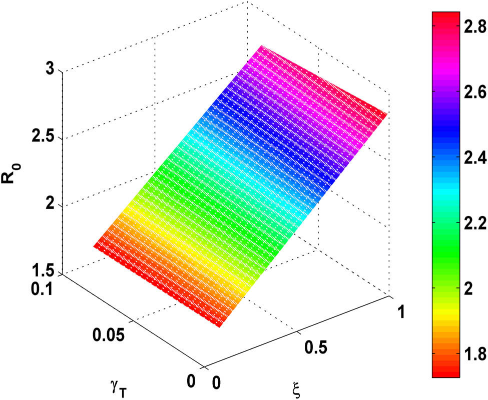
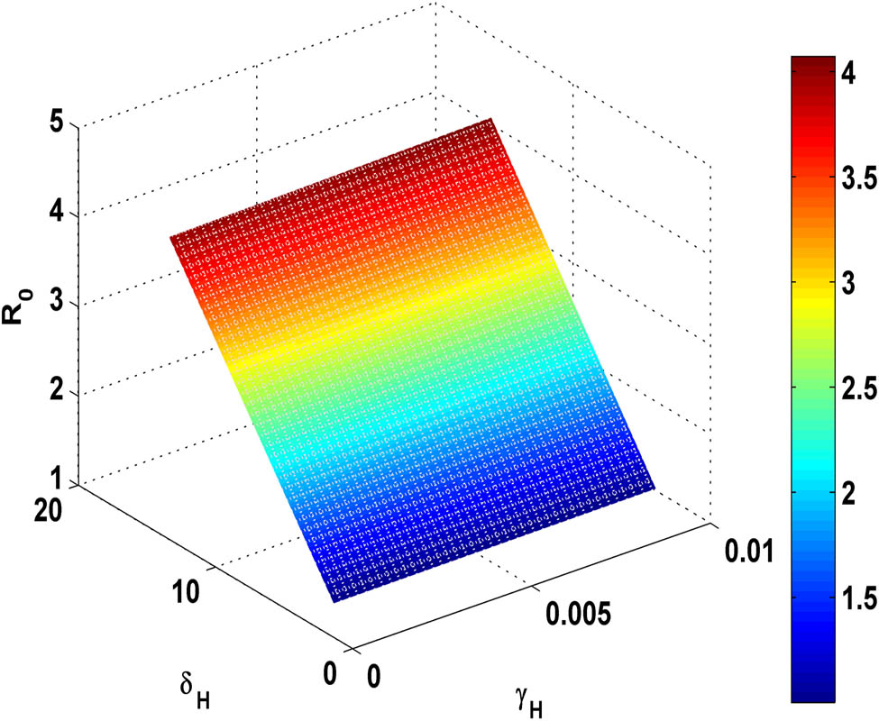
Figure 4 illustrates that the increment in the value of γ T magnifies R 0 more rapidly than ψ . When we increase ψ i.e., rate of lossing immunity after TB recovery of the individual, the value of fuzzy reproduction number R 0 T increases, γ T increases.

$Figure 4 Variation of R 0 {R}_{0} with the (fuzzy parameter) γ T {\gamma }_{T} and ψ \psi .$

Figure 4

Variation of R 0 with the (fuzzy parameter) γ T and ψ .

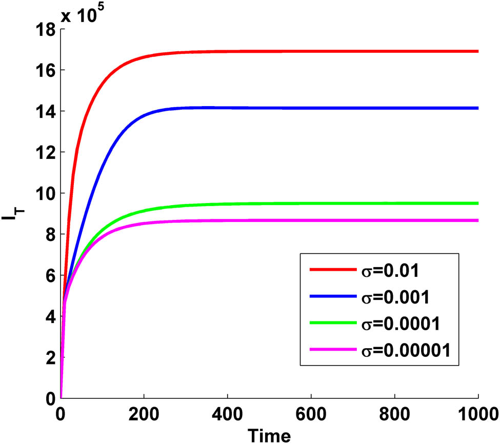
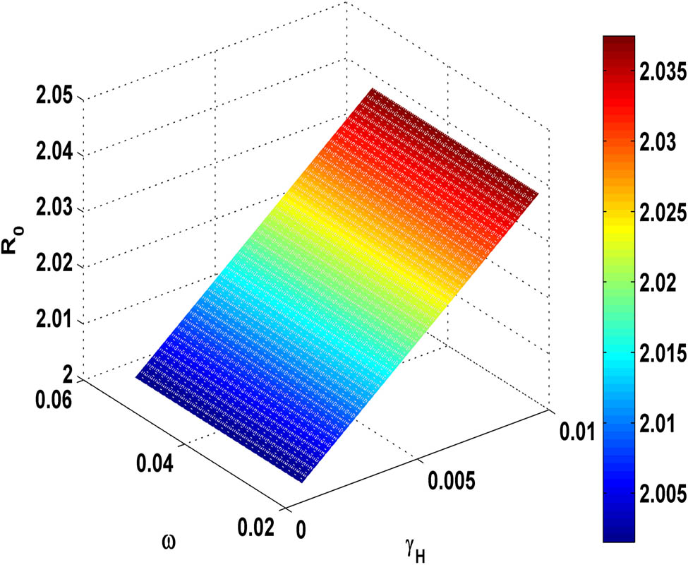
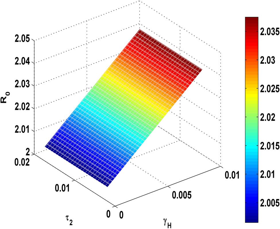
Figure 5 shows that as the value of γ T and Λ increases, the value of fuzzy reproduction number R 0 also increases. The shape of the plot indicates that γ T and Λ play a significant role in TB disease dynamics.

$Figure 5 Variation of R 0 H {R}_{{0}_{H}} with the (fuzzy parameter) γ T {\gamma }_{T} and Λ \Lambda .$

Figure 5

Variation of R 0 H with the (fuzzy parameter) γ T and Λ .

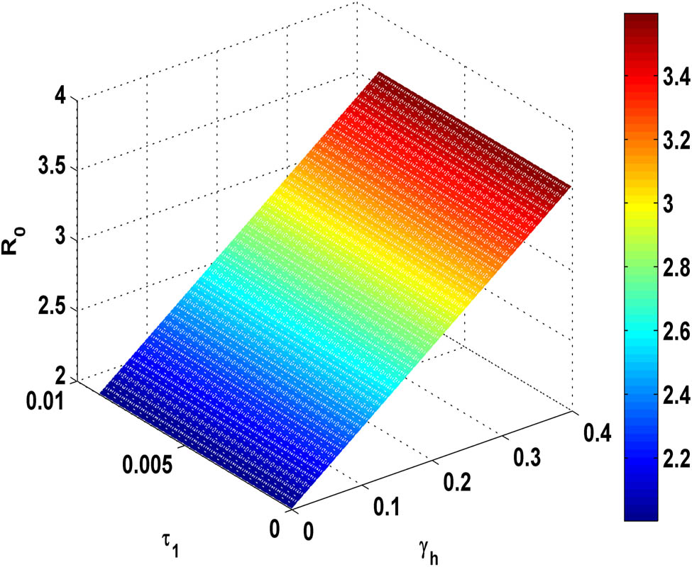
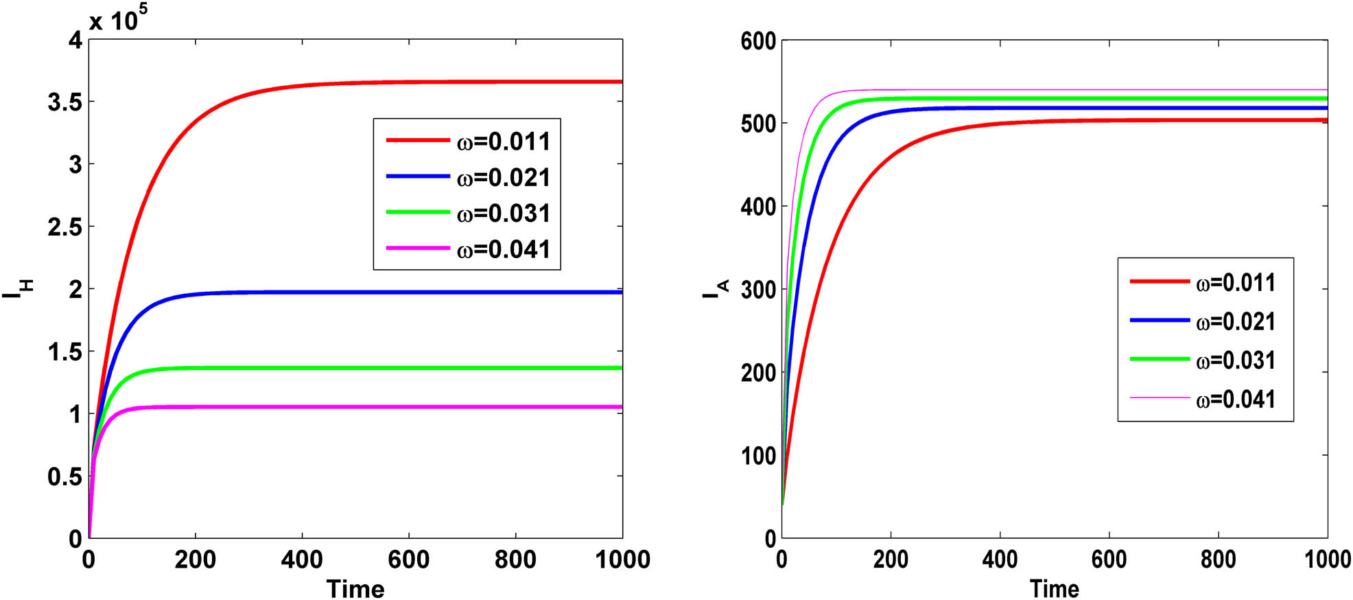
Figure 6 illustrates that as we increment in value of vaccination rate, ξ for susceptible population magnifies R 0 T more rapidly than TB transmission rate.

$Figure 6 Variation of R 0 {R}_{0} with the (fuzzy parameter) γ T {\gamma }_{T} and ξ \xi .$

Figure 6

Variation of R 0 with the (fuzzy parameter) γ T and ξ .

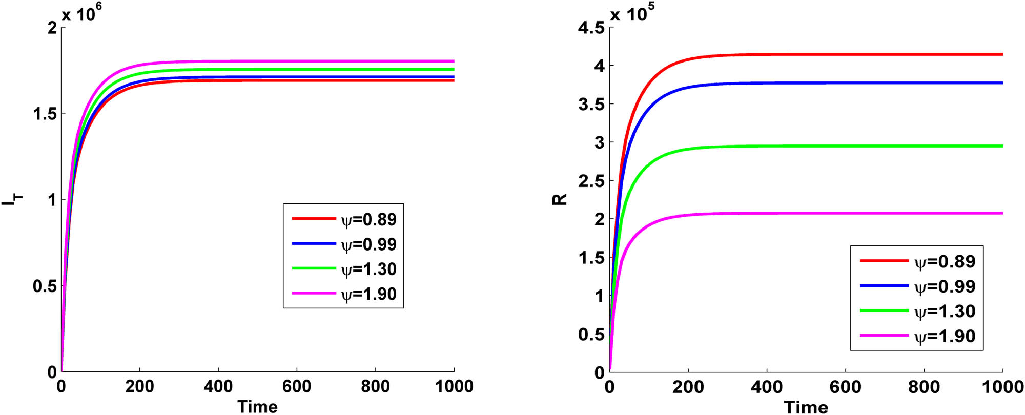
In Figure 7, we have drawn the variation of TB-infected population with time for HIV/AIDS infection. From the figure, we observe that as we increase the vaccine efficacy ( 1 − σ ) , then the infected decreases.

$Figure 7 Variation of I T {I}_{T} with time t t for different values of σ \sigma .$

Figure 7

Variation of I T with time t for different values of σ .

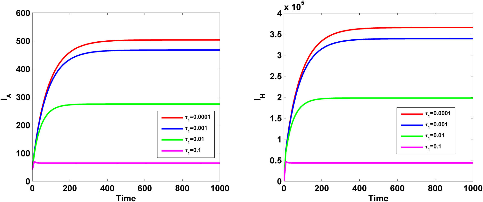
Figure 8 shows the variation of TB-infected population and recovered population with time for different values of ψ . From the left panel of this figure, it is seen that as we increase the rate of losing immunity after TB recovery, the behavior of the graph shows that infected population increases and recovered population decreases with time, which reveals that immunity should be provided to the population so that they can fight with the disease. From the right panel of this figure, it is seen that as we increase vaccine efficacy, the recovered population increases and the infected population decreases.

$Figure 8 Variation of I T {I}_{T} (left panel) and R (right panel) with time t t for different values of ψ \psi .$

Figure 8

Variation of I T (left panel) and R (right panel) with time t for different values of ψ .

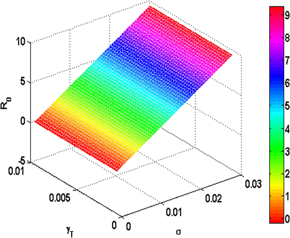
Figure 9 illustrates that as the value of effective transmission rate γ H of HIV-infected population and recruitment rate A of the susceptible population increases, then the value of fuzzy reproduction number R 0 H also increases.

$Figure 9 Variation of R 0 {R}_{0} with the (fuzzy parameter) γ H {\gamma }_{H} and Λ \Lambda .$

Figure 9

Variation of R 0 with the (fuzzy parameter) γ H and Λ .

Figure 10 demonstrates that if the transmission rate γ H of HIV-infected population and, the death rate of HIV-infected population increases, then fuzzy BRN R 0 H also increases.

$Figure 10 Variation of R 0 {R}_{0} with the (fuzzy parameter) γ H {\gamma }_{H} and (fuzzy parameter) δ H {\delta }_{H} .$

Figure 10

Variation of R 0 with the (fuzzy parameter) γ H and (fuzzy parameter) δ H .

Figure 11 shows that as the value of transmission rate γ H of HIV-infected population and the HIV progression rate ω increases, then the fuzzy BRN R 0 H also increases.

$Figure 11 Variation of R 0 {R}_{0} with the (fuzzy parameter) γ H {\gamma }_{H} and ω \omega .$

Figure 11

Variation of R 0 with the (fuzzy parameter) γ H and ω .

Figure 12 demonstrates that as the proportion τ 1 of HIV-infected population selected from I H to I A and effective transmission rate γ H of HIV/AIDS increases, then R 0 H increases.

$Figure 12 Variation of R 0 {R}_{0} with the (fuzzy parameter) γ H {\gamma }_{H} and τ 1 {\tau }_{1} .$

Figure 12

Variation of R 0 with the (fuzzy parameter) γ H and τ 1 .

Figure 13 demonstrates that as the proportion τ 2 of HIV-infected population with no symptoms of AIDS and effective transmission rate γ H of HIV/AIDS increases, the R 0 H increases.

$Figure 13 Variation of R 0 {R}_{0} with the (fuzzy parameter) γ H {\gamma }_{H} and τ 2 {\tau }_{2} .$

Figure 13

Variation of R 0 with the (fuzzy parameter) γ H and τ 2 .

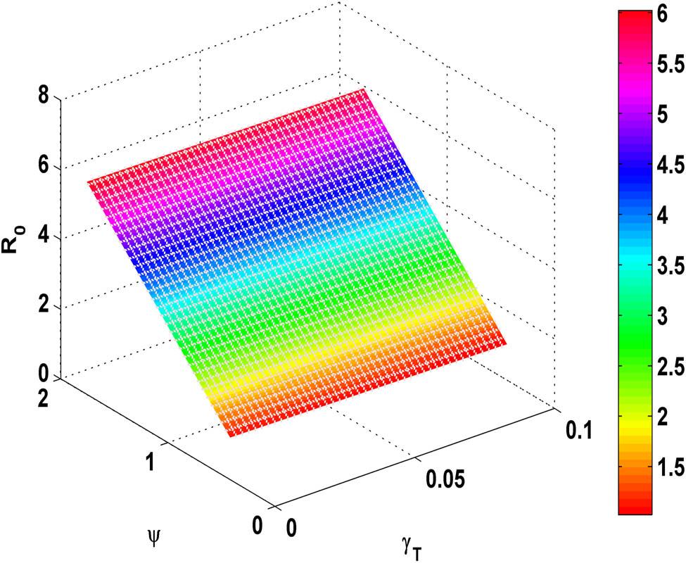
Figure 14 demonstrates that as the HIV progression rate ω increases, then HIV-infected population I H decreases resulting I A to be increasing.

$Figure 14 Variation of I H {I}_{H} (left panel) and I A {I}_{A} (right panel) with time t t for different values of ω \omega .$

Figure 14

Variation of I H (left panel) and I A (right panel) with time t for different values of ω .

Figure 15 demonstrates the variation of both HIV-infected population I H and AIDS-infected population I A with proportion rate τ 1 of HIV-infected population selected from I H to I A .

$Figure 15 Variation of I H {I}_{H} (leftt panel )and I A {I}_{A} (right panel) with time t t for different values of τ 1 {\tau }_{1} .$

Figure 15

Variation of I H (leftt panel )and I A (right panel) with time t for different values of τ 1 .

8 Conclusion

In this study, we have presented a co-infection model of HIV/AIDS and TB using fuzzy parameters. We have assumed that the infection is not spread uniformly among individuals in the entire population. Similarly, the recovery and death rates are also assumed to vary per individual. We have treated the HIV/AIDS and TB transmission rates γ H ( ν ) and γ T ( ν ) as fuzzy variables, the recovery rate as θ ( ν ) , and the death rate as δ H ( ν ) and δ T ( ν ) , respectively, as a function of viral concentration. In the model without fuzzy, the model parameters are unaffected by virus load, whereas the fuzzy model may be considered more adaptable and balanced. Fuzzy theory is utilized to deal with uncertainty quantification problems associated with mathematical disease modeling. We have tested it for various virus loads because fuzzy variables are virus load functions that vary with virus concentration. In light of this, we addressed the model’s fuzzy equilibrium points while taking into account various virus levels in the population. We have determined that the DFE point is attained when the virus concentration is less than the minimum concentration required for disease transmission in the population. When viral levels in the population exceeded the minimum required for disease transmission, we have attained endemic equilibrium. The basic reproduction rate is investigated at different virus concentrations. We have used the predicted value of a fuzzy number to obtain the fuzzy BRN. Three numerical schemes, namely, the Euler approach, the Runge–Kutta method of order 4, and the NSFD scheme, are established to approximate the solution of the examined model. The generated systems are tested for various amounts of virus. The proposed numerical techniques preserve the positive nature of the solutions to such dynamic population models. The proposed NSFD scheme is found to be unconditionally convergent and consistent. The current work focuses on developing, applying, and analyzing a NSFD technique for numerically analyzing the TB and HIV/AIDS co-infection model with fuzzy parameters. Future developments could include fuzzy stochastic, fuzzy delayed, or fuzzy fractional dynamic senses. The NSFD modeling theory could be applied to age-structured fuzzy epidemic models. The majority of this research focuses on representing membership functions with triangular fuzzy numbers. In the future, we may investigate the usage of various fuzzy numbers as potential membership functions, including trapezoidal, pentagonal, and hexagonal. Also in the future, this study could be enhanced in a variety of ways, such as combining fuzzy stochastic, fuzzy delayed, and fuzzy fractional dynamic aspects, as well as taking into account saturated incidence, treatment effects, and delays with fuzzy parameters. Furthermore, the NSFD modeling theory might be expanded to include age-structured fuzzy epidemic models, as well as study a number of other possibilities.

Acknowledgments

The researchers would like to thank the Deanship of Graduate Studies and Scientific Research at the Qassim University for financial support (QU-APC-2025).

Funding information: The researchers would like to thank the Deanship of Graduate Studies and Scientific Research at the Qassim University for financial support (QU-APC-2025).
Author contributions: All Authors have equally contributed to this paper.
Conflict of interest: The authors state no conflict of interest.
Data availability statement: The datasets used and/or analyzed during the curent study available from the corresponding author on reasonable request.

References

[1] Jain S, El-Khatib Y. Modelling chaotic dynamical attractor with fractal-fractional differential operators. AIMS Math. 2021 Jan 1;1(12):13689–725. 10.3934/math.2021795Search in Google Scholar

[2] Jain S. Numerical analysis for the fractional diffusion and fractional Buckmaster equation by the two-step Laplace Adam-Bashforth method. Europ Phys J Plus. 2018 Jan 19;133(1):19. 10.1140/epjp/i2018-11854-xSearch in Google Scholar

[3] Owolabi KM, Jain S. Spatial patterns through diffusion-driven instability in modified predator-prey models with chaotic behaviors. Chaos Solitons Fractals. 2023;174:113839. Search in Google Scholar

[4] Owolabi KM, Jain S. Spatial patterns through diffusion-driven instability in modified predator-prey models with chaotic behaviors. Chaos Solitons Fractals. 2023 Sep 1;174:113839. 10.1016/j.chaos.2023.113839Search in Google Scholar

[5] Atangana A, Jain S. The role of power decay, exponential decay and Mittag-Leffler function’s waiting time distribution: application of cancer spread. Phys A Stat Mech Appl. 2018 Dec 15;512:330–51. 10.1016/j.physa.2018.08.033Search in Google Scholar

[6] Brauer F, Castillo-Chavez C, Castillo-Chavez C. Mathematical models in population biology and epidemiology. New York: Springer; 2012. 10.1007/978-1-4614-1686-9Search in Google Scholar

[7] Verma AK, Kayenat S. On the convergence of Mickens’ type nonstandard finite difference schemes on Lane-Emden type equations. J Math Chem. 2018 Jun;56:1667–706. 10.1007/s10910-018-0880-ySearch in Google Scholar

[8] Conte D, Guarino N, Pagano G, Paternoster B. On the advantages of nonstandard finite difference discretizations for differential problems. Numer Anal Appl. 2022 Sep;15(3):219–35. 10.1134/S1995423922030041Search in Google Scholar

[9] Mickens RE. Advances in the applications of nonstandard finite difference schemes. Singapore: World Scientific; 2005 Oct 25. 10.1142/9789812703316Search in Google Scholar

[10] Cresson J, Pierret F. Non standard finite difference scheme preserving dynamical properties. J Comput Appl Math. 2016 Sep 1 303:15–30. 10.1016/j.cam.2016.02.007Search in Google Scholar

[11] Goguen JA, Zadeh LA. Fuzzy sets. Information and control. 1965;8:338–53. Zadeh LA. Similarity relations and fuzzy orderings. Information sciences, vol. 3 (1971), pp. 177-200. J Symb Log. 1973 Dec;38(4):656–7. 10.2307/2272014Search in Google Scholar

[12] Mondal PK, Jana S, Haldar P, Kar TK. Dynamical behavior of an epidemic model in a fuzzy transmission. Int J Uncertainty Fuzziness Knowl-Based Syst. 2015 Oct;23(05):651–65. 10.1142/S0218488515500282Search in Google Scholar

[13] Lefevr N, Kanavos A, Gerogiannis VC, Iliadis L, Pintelas P. Employing fuzzy logic to analyze the structure of complex biological and epidemic spreading models. Mathematics. 2021 Apr 27;9(9):977. 10.3390/math9090977Search in Google Scholar

[14] Vos T. Global burden of 369 diseases and injuries in 204 countries and territories, 1990-2019: a systematic analysis for the Global Burden of Disease Study 2019 (vol. 396, p. 1204, 2020). Lancet. 2020 Nov 14;396:(10262):1562. Search in Google Scholar

[15] Batu TD, Obsu LL, Deressa CT. Co-infection dynamics of COVID-19 and HIV/AIDS. Scientif Reports. 2023 Oct 27;13(1):18437. 10.1038/s41598-023-45520-6Search in Google Scholar PubMed PubMed Central

[16] WHO. Global HIV Programme 2020 estimates. 2022. https://bit.ly/3HmxDpQ. Search in Google Scholar

[17] Maartens G, Celum C, Lewin SR. HIV infection: epidemiology, pathogenesis, treatment, and prevention. The Lancet. 2014 Jul 19;384(9939):258–71. 10.1016/S0140-6736(14)60164-1Search in Google Scholar PubMed

[18] Morison L. The global epidemiology of HIV/AIDS. British Med Bulletin. 2001 Sep 1;58(1):7–18. 10.1093/bmb/58.1.7Search in Google Scholar PubMed

[19] Simon V, Ho DD, Karim QA. HIV/AIDS epidemiology, pathogenesis, prevention, and treatment. The Lancet. 2006 Aug 5;368(9534):489–504. 10.1016/S0140-6736(06)69157-5Search in Google Scholar PubMed PubMed Central

[20] d’Arminio Monforte A, Cozzi-Lepri A, Castagna A, Antinori A, De Luca A, Mussini C, et al. Risk of developing specific AIDS-defining illnesses in patients coinfected with HIV and hepatitis C virus with or without liver cirrhosis. Clin Infect Diseases. 2009 Aug 15;49(4):612–22. 10.1086/603557Search in Google Scholar PubMed

[21] Centers for disease control and prevention. Evidence of HIV treatment and viral suppression in preventing the sexual transmission of HIV. Dep Heal Hum Serv. 2018 Dec;4:15. Search in Google Scholar

[22] Rwezaura H, Diagne ML, Omame A, de Espindola AL, Tchuenche JM. Mathematical modeling and optimal control of SARS-CoV-2 and tuberculosis co-infection: a case study of Indonesia. Model Earth Syst Environ. 2022 Nov;8(4):5493–520. 10.1007/s40808-022-01430-6Search in Google Scholar PubMed PubMed Central

[23] World Health Organisation. www.who.int/tb/publications/glob-al_report/en/. Search in Google Scholar

[24] World Health Organisation. www.who.int/news-room/fact-sheets/detail/tuberculosis. Search in Google Scholar

[25] Centers for disease control and prevention. www.cdc.gov/tb/topic/basics/tbinfectiondisease.htm. Search in Google Scholar

[26] Magdaleno D, Montes M, Estrada B, Ochoa-Zezzatti A. A GPT-based approach for sentiment analysis and bakery rating prediction. InMexican International Conference on Artificial Intelligence. Cham: Springer Nature Switzerland; 2023 Nov 13. pp. 61–76. 10.1007/978-3-031-51940-6_7Search in Google Scholar

[27] Tilahun GT. Modeling co-dynamics of pneumonia and meningitis diseases. Adv Differ Equ. 2019 Dec;2019(1):1–8. 10.1186/s13662-019-2087-3Search in Google Scholar

[28] Omame A, Okuonghae D, Umana RA, Inyama SC. Analysis of a co-infection model for HPV-TB. Appl Math Model. 2020 Jan 1;77:881–901. 10.1016/j.apm.2019.08.012Search in Google Scholar

[29] Varshney KG, Dwivedi YK. Mathematical modeling of influenza-meningitis under the quarantine effect of influenza. Turkish J Comput Math Educ. 2021;12(11):7214–25. Search in Google Scholar

[30] Omame A, Okuonghae D. A co-infection model for oncogenic human papillomavirus and tuberculosis with optimal control and cost-effectiveness analysis. Opt Control Appl Methods. 2021 Jul;42(4):1081–101. 10.1002/oca.2717Search in Google Scholar

[31] Faniran TS, Adewole MO, Ahmad H, Abdullah FA. Dynamics of tuberculosis in HIV-HCV co-infected cases. Int J Biomath. 2023 Apr 28;16(3):2250091. 10.1142/S1793524522500917Search in Google Scholar

[32] Sil N, Mahata A, Roy B. Dynamical behavior of HIV infection in fuzzy environment. Results Control Optim. 2023 Mar 1;10:100209. 10.1016/j.rico.2023.100209Search in Google Scholar

[33] Melin P, Castillo O. Spatial and temporal spread of the COVID-19 pandemic using self organizing neural networks and a fuzzy fractal approach. Sustainability. 2021 Jul 24;13(15):8295. 10.3390/su13158295Search in Google Scholar

[34] Castillo O, Melin P. A new fuzzy fractal control approach of non-linear dynamic systems: The case of controlling the COVID-19 pandemics. Chaos Solitons Fractals. 2021 Oct 1;151:111250. 10.1016/j.chaos.2021.111250Search in Google Scholar PubMed PubMed Central

[35] Ahmed N, Shahid N, Iqbal Z, Jawaz M, Rafiq M, Tahira SS, et al. Numerical modeling of SEIQV epidemic model with saturated incidence rate. J Appl Environ Biol Sci. 2018;8(4):67–82. Search in Google Scholar

[36] De Barros LC, Bassanezi RC, Lodwick WA. First course in fuzzy logic, fuzzy dynamical systems, and biomathematics. Berlin: Springer-Verlag: 2016. 10.1007/978-3-662-53324-6Search in Google Scholar

[37] Liu B, Liu YK. Expected value of fuzzy variable and fuzzy expected value models. IEEE Trans Fuzzy Syst. 2002 Aug;10(4):445–50. 10.1109/TFUZZ.2002.800692Search in Google Scholar

[38] Mangongo YT, Bukweli JD, Kampempe JD. Fuzzy global stability analysis of the dynamics of malaria with fuzzy transmission and recovery rates. Am J Operat Res. 2021 Oct 13;11(6):257–82. 10.4236/ajor.2021.116017Search in Google Scholar

[39] Salahshour S, Ahmadian A, Mahata A, Mondal SP, Alam S. The behavior of logistic equation with alley effect in fuzzy environment: fuzzy differential equation approach. Int J Appl Comput Math. 2018 Apr;4:1–20. 10.1007/s40819-018-0496-8Search in Google Scholar

[40] Panda A, Pal M. A study on pentagonal fuzzy number and its corresponding matrices. Pacific Sci Rev B Human Soc Sc. 2015 Nov 1;1(3):131–9. 10.1016/j.psrb.2016.08.001Search in Google Scholar

Received: 2024-07-22

Revised: 2025-03-10

Accepted: 2025-04-01

Published Online: 2025-06-02

This work is licensed under the Creative Commons Attribution 4.0 International License.

Articles in the same Issue

https://doi.org/10.1515/nleng-2025-0131

Keywords for this article

tuberculosis and HIV/AIDS; fuzzy environment; forward Euler’s method; Runge–Kutta method; finite difference scheme; numerical methods; mathematical model

Creative Commons

BY 4.0