Numerical computational model for an unsteady hybrid nanofluid flow in a porous medium past an MHD rotating sheet
-
 and
and

Abstract
This article presents a study of a rotating hybrid nanofluid flow in a porous medium past a stretching surface using an overlapping grid multi-domain bivariate spectral simple iteration method (OMD-BSSIM). The objective is to appraise the performance of the OMD-BSSIM on a system of nonlinear partial differential equations that describe the unsteady flow of a hybrid nanofluid composed of copper and aluminum oxide nanoparticles in water. Additionally, the study aims to evaluate the impact of different fluid and surface parameters on the behavior of the hybrid nanofluid. The improved OMD-BSSIM algorithm is implemented in MATLAB and tested for its convergence and accuracy. The results are compared with previously published findings that were obtained using the overlapping spectral local linearization method and the bivariate spectral relaxation method. The study explores the use of R line graphs as a visualization tool to identify patterns and relationships among the skin friction coefficients, local Nusselt number, and local Sherwood number of the hybrid nanofluid and parameters over time. The findings reveal several key trends and patterns, such as the positive correlation between the shrinking ratio parameter and the skin friction coefficient and the positive relationship between increasing the rotation parameter and an inverse relationship between an increase in the alumina volume fraction coefficient and the local Nusselt number of the hybrid nanofluid. This article provides valuable insights into the flow behavior of hybrid nanofluids and highlights the potential of alumina nanoparticles as a tool for enhancing the thermal and mechanical properties of the fluid.
Nomenclature
-
-
Cartesian coordinate system
-
-
velocities in direction
-
-
time
-
-
hybrid nanofluid temperature
-
-
ambient temperature
-
-
wall temperature
-
-
hybrid nanofluid concentration
-
-
ambient concentration
-
-
wall concentration
-
-
magnetic field coefficient
-
-
heat generation/absorption coefficient
-
-
specific heat capacity
-
-
acceleration due to gravity
-
-
shrinking parameters
-
-
velocity components after transformation
-
Greek symbols
-
-
density
-
-
heat generation/absorption parameter
-
-
porosity parameter
-
-
dynamic viscosity
-
-
electrical conductivity
-
-
angular velocity
-
-
rotation parameter
-
-
thermal conductivity
-
-
chemical reaction parameter
-
-
nanoparticle volume fraction
-
-
stretching/shrinking ratio parameter
-
-
coordinate for transformation space
-
-
coordinate for transformation time
-
-
non-dimensional temperature
-
-
non-dimensional concentration
-
Subscripts
-
-
alumina nanoparticle
-
-
copper nanoparticle
-
-
base fluid
-
-
nanofluid
-
-
hybrid nanofluid
-
Abbreviations
- S
-
total number of the grid points
- T
-
vector transpose
- BCs
-
boundary conditions
- MHD
-
magnetohydrodynamic
- SIM
-
simple iteration method
- LLM
-
local linearization method
- OMD
-
overlapping grid multi-domain
- SSIM
-
spectral simple iteration method
- SLLM
-
spectral local linearization method
- BSRM
-
bivariate spectral relaxation method
1 Introduction
Hybrid nanofluids are a popular research topic due to, among other uses, their ability to improve heat transfer, thermal conductivity, and filtration efficiency [1]. Nanoparticles can be made from a variety of materials [2,3]. Adding nanoparticles to a liquid has been shown to improve electrical, thermal, and acoustical conductivity. Hybrid nanofluids consist of a base fluid and a mixture of nanoparticles [4]. The most commonly used base fluids include water, organic liquids, oils, bio-fluids, and polymeric solutions [5]. Numerous experiments and numerical simulations have demonstrated that nanofluids and hybrid nanofluids have high heat transfer efficiency compared to base fluids. However, researchers continue to push the boundaries of research in this area to expand knowledge. For example, some studies have explored the use of two different types of nanoparticles in nanofluids, rather than one type of particle. In addition, researchers have examined the impact of external factors, such as electric and magnetic fields, the effects of porous media, shrinking or stretching plates, and temperature, on the motion and heat transfer of hybrid nanofluids.
The field of magnetohydrodynamics (MHD) was first formally introduced by Alfvén [6]. MHD studies primarily focus on the dynamics and behavior of electrically conductive fluid, with particular emphasis on heat transfer management. The pioneering investigation of convective flow past a stretching sheet was conducted by Crane [7]. Many other studies have subsequently explored different aspects of the stretching sheet problem [8,9]. In manufacturing processes that involve stretching surfaces, it is crucial to take into account how the sheet is stretched and how heat within it is controlled. The dynamics of fluid motion through porous media has garnered significant attention. Understanding the nuances of fluid flow through porous media has ramifications for fields such as hydro-geology and petroleum engineering [10]. This requires an in-depth understanding of the intricate interplay among the fluid, the porous material, and the array of forces that govern and influence the flow through these intricate pathways. In this work, we combine the study of MHD effects with the impact of nanoparticles on a stretching surface. Despite the progress made in this fields, there is still a lot to learn about the mechanisms behind the enhanced heat transfer rates of hybrid nanofluids. This article aims to contribute to this understanding by studying the flow of hybrid nanofluids and examining the influence of external factors on their heat transfer properties.
Khalili et al. [11] performed a numerical investigation of the flow and heat transfer characteristics of nanofluids consisting of copper (Cu), titanium dioxide (
Khan et al. [14] recently investigated the behavior of ferrous oxide (
Despite the extensive investigations on hybrid nanofluids, to the best of our knowledge, there has been no attempt to find a numerical solution for the three-dimensional unsteady hybrid nanofluid flow. To address this gap, we model the MHD rotating flow of an
Recently, Mkhatshwa et al. [18,19] proposed an improvement of the standard algorithm for solving N-PDEs by introducing a novel overlapping grid multi-domain bivariate spectral quasi-linearization method (OMD-BSQLM) and the overlapping multi-domain bivariate spectral local linearization method (OMD-BSLLM). The solution algorithm involves linearizing and decoupling the N-PDEs using a uni-variate linearization technique along with a spectral collocation discretization. The methods have been successfully applied to solve various flow problems, including models for hybrid nanofluid flows. The combination of the overlapping technique with the bivariate spectral method has been demonstrated to provide accurate solutions [20]. The overlapping grid multi-domain method is used to solve N-PDEs involving two independent variables, namely space and time. The approach involves dividing the time domain into distinct, non-overlapping sub-domains, while the space domain is divided into sub-domains that overlap with each other. The overlapping techniques that have been developed guarantee a matrix with fewer elements and require a smaller number of grid points [17].
This article presents the overlapping grid multi-domain bivariate spectral simple iteration method (OMD-BSSIM) for finding numerical solutions to a system of N-PDEs that model unsteady hybrid nanofluid flow problems. The OMD-BSSIM is extended to the OMD-BSLLM by applying the simple iteration technique (SIM) instead of the local linearization technique (LLM). The method is modified to achieve computational efficiency. Linearization based on truncated Taylor series approximations is employed to simplify terms in the nonlinear differential equations [21]. The LLM, quasi-linearization method, and Keller-box methods are based on a one-term Taylor series expansion and are therefore susceptible to truncation errors. The relaxation method (RM) technique is based on the assumption that the non-linear terms are known from previous iterations. The SIM uses ideas akin to those of fixed-point iteration as an iterative scheme. Both the SIM and LLM techniques were proposed by Motsa et al. [22,23]. The effectiveness of the SIM is validated by comparison with the finite difference method for boundary-value problems [24].
2 Mathematical model
Consider the unsteady MHD flow of an incompressible, electrically conducting, rotating, stratified Cu-
subject to the boundary conditions (BCs)
The linearly shrinking velocities at the surface are defined by
respectively. In Eqs. (1)–(6),

Geometry configuration of the problem.
Table 1 shows the thermophysical properties of
| Physical properties |
|
Cu |
|
|---|---|---|---|
|
|
|
|
|
|
|
0.05 |
|
|
|
|
997.1 | 8,933 | 3,970 |
|
|
0.613 | 400 | 40 |
|
|
4179 | 385 | 765 |
| Properties | Nanofluid | Hybrid nanofluid |
|---|---|---|
| Density |
|
|
| Dynamic viscosity |
|
|
| Electrical conductivity |
|
|
| Heat capacity |
|
|
| Mass diffusivity |
|
|
| Thermal conductivity |
|
|
| Thermal expansion |
|
|
Eqs. (1)–(6) are transformed into a non-dimensional form [25,32,33] using
Eq. (1) is satisfied identically using the above similarity transformations. Substituting Eq. (10) into Eqs. (2)–(6) yields
Here,
where
The parameter Ri is the local Richardson number, Gr is the local Grashof number, Re is the local Reynolds number, Pr is the Prandtl number, and Sc is the Schmidt number, which are defined as
The physical quantities of interest are skin friction coefficients along the
3 Method of solution
In this section, we develop the iterative OMD-BSSIM scheme for the solution of the flow Eqs. (11)–(14) together with the BCs (15)–(16). The solution algorithm encompasses two fundamental components: the linearization of the N-PDEs utilizing the SIM technique and the incorporation of Chebyshev bivariate spectral collocation discretization.
3.1 SIM
In the SIM implementation, we consider the nonlinear terms as a combination of known (at iteration
In Eqs. (18)–(21), the coefficients
3.2 Chebyshev differentiation
The main feature of the OMD-Chebyshev spectral collocation method is the use of an overlapping grid procedure in the space variable (

Non-overlapping grid (
Figure 3 displays the sub-division of the overlapping space domain
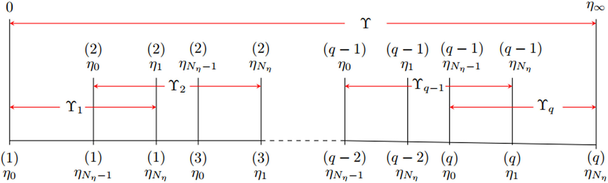
Overlapping grid (
We transform the sub-intervals
The functions
The matrix
The time derivatives are computed as
The matrix
where the superscript
Substituting Eqs. (22)–(30) into Eqs. (18)–(21), we obtain
Equations (31)–(34) represent the subsystem expressed as matrices of size
and
The functions taken as guesses for initiating the iteration procedure are
which are chosen to satisfy the BC equations (35)–(37). After imposing the BC equations (35)–(37) into the matrix subsystems (31)–(34), the solutions are derived through solving the matrix systems iteratively
where
It can be seen that when
Applying the overlapping grid on the spatial variable (
4 Results and discussion
To verify the accuracy of the SIM method, we utilized the O-SLLM and O-SSIM to solve Eqs. (43)–(46). Table 3 presents a comparison and validation demonstrating the clear consistency of the SIM. We used
Comparison of overlapping SSIM for values of
| Pr | Devi and Devi [35] | Khashii’ie et al. [36] | Waini et al. [37] | O-SLLM [16] | O-SSIM |
|---|---|---|---|---|---|
| 2.00 | 0.91135 | 0.91135 | 0.911357 | 0.91135276 | 0.9113527637 |
| 6.13 | 1.75968 | 1.75968 | 1.759682 | 1.75968170 | 1.7596817080 |
| 7.00 | 1.89540 | 1.89540 | 1.895400 | 1.89540040 | 1.8954004012 |
| 20.0 | 3.35390 | 3.35390 | 3.353893 | 3.35390184 | 3.3538961832 |
| CPU time (s) | — | — | — | 0.052554 | 0.041551 |
Equations (11)–(14) were solved numerically using the OMD-BSSIM. Table 4 shows
Comparison of implementation the OMD-BSSIM when
|
|
|
|
|
|||||
|---|---|---|---|---|---|---|---|---|
|
|
BSRM [33] | Present | BSRM [33] | Present | BSRM [33] | Present | BSRM [33] | Present |
| 0.1 |
|
|
|
|
|
|
|
|
| 0.3 |
|
|
|
|
|
|
|
|
| 0.5 |
|
|
|
|
|
|
|
|
| 0.7 |
|
|
|
|
|
|
|
|
| 0.9 |
|
|
|
|
|
|
|
|
The numerical computations are executed using the values
unless indicated otherwise. We examined the residual errors and the solution errors for different values of
Table 5 and Figure 4 present the residual errors for different values of
Table 6 illustrates how increasing the number of overlapping sub-intervals impacts the errors in the solution. We remark that when
Residual errors at
|
|
|
|
|
|
|
|
CPU time in seconds |
|---|---|---|---|---|---|---|---|
| 120 | 1 | 120 |
|
|
|
|
1.004388 |
| 20 | 5 | 96 |
|
|
|
|
0.891982 |
| 9 | 9 | 73 |
|
|
|
|
0.829143 |
| 4 | 15 | 46 |
|
|
|
|
0.767800 |

The residual error graphs of the OMD-BSSIM solution when
Convergence of the solutions
|
|
|
|
|
|
|
|
|---|---|---|---|---|---|---|
| 120 | 1 | 120 |
|
|
|
|
| 20 | 5 | 96 |
|
|
|
|
| 9 | 9 | 73 |
|
|
|
|
| 4 | 15 | 46 |
|
|
|
|
Figure 5 illustrates the numerical values of velocity, temperature, and concentration functions when

The numerical solution utilized the OMD-BSSIM. (a) Numerical solution of
We investigated the effect of the shrinking and stretching parameter (
Figure 6 shows the influence of the shrinking and stretching parameter, the porosity parameter, the magnetic parameter, and the volume fraction of aluminum oxide nanoparticle parameters on the velocity in the

Velocity profiles in the

Velocity profiles in the
Figure 8 shows the effect of the shrinking and stretching parameter, the porosity parameter, the rotation parameter, and the volume fraction of aluminum oxide nanoparticles on temperature. Figure 8(a) depicts that the temperature of the hybrid nanofluid flow increases with the shrinking parameter but decreases with the stretching parameter. The temperature of the hybrid nanofluid flow increases due to heat conduction from the surface, which can cause changes in density and viscosity. Figure 8(b) indicates that increasing the porosity parameter improves temperature distribution. Higher porosity can lead to lower thermal conductivity and viscosity of the fluid, resulting in reduced heat transfer. However, it should be noted that the presence of nanoparticles can enhance heat transfer by increasing the effective thermal conductivity and convective heat transfer coefficient of the hybrid nanofluid. Nevertheless, if the nanoparticles agglomerate and form blockages, they can reduce the flow rate, leading to a higher fluid temperature. Figure 8(c) shows that the temperature profile increases with the introduction of the rotation parameter. This is because increased rotation can induce higher shear rates in the hybrid nanofluid, leading to increased viscous dissipation and heating of the fluid. Figure 8(d) shows that temperature improves as the value of the volume fraction of aluminum oxide nanoparticles increases. This increase in thermal conductivity can reduce the thermal boundary layer and improve the heat transfer rate.

Temperature profiles at
The effect of the shrinking and stretching parameter, the chemical reaction parameter, the Schmidt number, and the volume fraction of copper nanoparticles on the concentration profile, is illustrated in Figure 9. Figure 9(a) shows that the concentration of the hybrid nanofluid increases with the shrinking of the boundary layer and decreases with the stretching of the boundary layer. The concentration profile becomes more uniform due to increased mixing caused by turbulence and the thickness of the boundary layer. Figure 9(b) demonstrates that increasing chemical reaction parameter leads to a reduction in concentration. This is because the reaction will consume the nanoparticles in regions where the reaction is more active, leading to a decrease in the local concentration of nanoparticles. This effect can be more significant in regions where the reaction rate is high. Figure 9(c) reveals that the concentration decreases with an increase in the Schmidt number value. The Schmidt number is a dimensionless parameter that represents the ratio of momentum diffusivity to mass diffusivity in a fluid. It describes the transport of a passive scalar, such as the concentration of nanoparticles in a hybrid nanofluid. Increasing the Schmidt number leads to decreased mixing and slower transport of nanoparticles in the fluid. Figure 9(d) indicates a rising trend in concentration with increasing values of volume fraction of copper nanoparticles. However, it can be seen that the change in concentration is small.

Concentration profiles at
This study also aims to examine how the copper and aluminum oxide fraction coefficients, shrinking ratio, rotation, and magnetic parameters relate to the skin friction coefficients (

OMD-SSIM for
5 Conclusion
The study presented the development of the OMD-BSSIM to solve model equations for the unsteady three-dimensional MHD flow of an incompressible, electrically conducting, rotating Cu-
The OMD-BSSIM may be used in both small and large computational domains.
The SIM requires less computational time than the LLM.
The incorporation of the overlapping grid approach contributes to improving the efficiency of the Chebyshev bivariate spectral collocation discretization.
The accuracy improves by increasing the number of the overlapping sub-intervals.
The OMD-BSSIM gives better solutions errors using a minimal number of grid points.
The analysis of residual errors highlights the significance of solution-updating strategies in improving the accuracy and convergence of the method.
Acknowledgments
The authors are grateful to the University of KwaZulu-Natal.
-
Funding information: Authors state no funding involved.
-
Author contributions: Salma Ahmedai: conceptualization, methodology, software, investigation, writing – original draft preparation. Precious Sibanda: validation, writing – review and editing, visualization, supervision. Sicelo P. Goqo: writing-review and editing, visualization, supervision. Osman A.I. Noreldin: writing-review and editing, visualization, supervision. All authors have accepted responsibility for the entire content of this manuscript and approved its submission.
-
Conflict of interest: Authors state no conflict of interest.
-
Data availability statement: All data generated or analysed during this study are included in this published article.
References
[1] Xu HJ, Xing ZB, Wang F, Cheng Z. Review on heat conduction, heat convection, thermal radiation and phase change heat transfer of nanofluids in porous media: Fundamentals and applications. Chem Eng Sci. 2019;195:462–83. 10.1016/j.ces.2018.09.045Search in Google Scholar
[2] Sarkar J, Ghosh P, Adil A. A review on hybrid nanofluids: recent research, development and applications. Renew Sustain Energy Rev. 2015;43:164–77. 10.1016/j.rser.2014.11.023Search in Google Scholar
[3] Muneeshwaran M, Srinivasan G, Muthukumar P, Wang CC. Role of hybrid-nanofluid in heat transfer enhancement-A review. Int Commun Heat Mass Transfer. 2021;125:105341. 10.1016/j.icheatmasstransfer.2021.105341Search in Google Scholar
[4] Li Y, Zhou J, Tung S, Schneider E, Xi S. A review on development of nanofluid preparation and characterization. Powder Tech. 2009;196(2):89–101. 10.1016/j.powtec.2009.07.025Search in Google Scholar
[5] Jahar S. A critical review on convective heat transfer correlations of nanofluids. Renew Sustain Energy Reviews. 2011;15(6):3271–7. 10.1016/j.rser.2011.04.025Search in Google Scholar
[6] Alfvén H. Existence of electromagnetic-hydrodynamic waves. Nature. 1942;150(3805):405–6. 10.1038/150405d0Search in Google Scholar
[7] Crane LJ. Flow past a stretching plate. Zeitschrift für angewandte Mathematik und Physik ZAMP. 1970;21:645–7. 10.1007/BF01587695Search in Google Scholar
[8] Chen CH. Effect of viscous dissipation on heat transfer in a non-Newtonian liquid film over an unsteady stretching sheet. J Non-Newton Fluid Mech. 2006;135(2–3):128–35. 10.1016/j.jnnfm.2006.01.009Search in Google Scholar
[9] Awan AU, Aziz M, Ullah N, Nadeem S, Abro KA. Thermal analysis of oblique stagnation point flow with slippage on second-order fluid. J Thermal Anal Calorimetry. 2021:147:3839–51. 10.1007/s10973-021-10760-zSearch in Google Scholar
[10] Yarlagadda A, Yoganathan A. Experimental studies of model porous media fluid dynamics. Experiments Fluids. 1989;8(1–2):59–71. 10.1007/BF00203066Search in Google Scholar
[11] Khalili S, Dinarvand S, Hosseini R, Tamim H, Pop I. flow and heat transfer near stagnation point over a stretching/shrinking sheet in porous medium filled with a nanofluid. Chin Phys B. 2014;23(4):048203. 10.1088/1674-1056/23/4/048203Search in Google Scholar
[12] Dinarvand S, Yousefi M, Chamkha A, et al. Numerical simulation of unsteady flow toward a stretching/shrinking sheet in porous medium filled with a hybrid nanofluid. J Appl Comput Mech. 2019;8:11–20. Search in Google Scholar
[13] Kierzenka J, Shampine LF. A BVP solver based on residual control and the Maltab PSE. ACM Trans Math Software (TOMS). 2001;27(3):299–316. 10.1145/502800.502801Search in Google Scholar
[14] Khan MS, Mei S, Shabnam, Fernandez-Gamiz U, Noeiaghdam S, Shah SA, et al. Numerical analysis of unsteady hybrid nanofluid flow comprising CNTs-ferrousoxide/water with variable magnetic field. Nanomaterials. 2022;12(2):180. 10.3390/nano12020180Search in Google Scholar PubMed PubMed Central
[15] Seydel R, Hlavacek V. Role of continuation in engineering analysis. Chem Eng Sci. 1987;42(6):1281–95. 10.1016/0009-2509(87)85001-7Search in Google Scholar
[16] Mkhatshwa M, Khumalo M. Irreversibility scrutinization on EMHD Darcy-Forchheimer slip flow of Carreau hybrid nanofluid through a stretchable surface in porous medium with temperature-variant properties. Heat Transfer. 2023;52(1):395–429. 10.1002/htj.22700Search in Google Scholar
[17] Mkhatshwa MP. Overlapping grid spectral collocation methods for nonlinear differential equations modelling fluid flow problems. [Ph.D. thesis 2020]. University of KwaZulu-Natal; 2023. Search in Google Scholar
[18] Mkhatshwa M, Motsa S, Sibanda P. Overlapping multi-domain bivariate spectral method for systems of nonlinear PDEs with fluid mechanics applications. In: Advances in Fluid Dynamics: Selected Proceedings of ICAFD 2018. Springer; 2021. p. 685–99. 10.1007/978-981-15-4308-1_54Search in Google Scholar
[19] Mkhatshwa M. Overlapping grid spectral collocation approach for electrical MHD bioconvection Darcy-Forchheimer flow of a Carreau-Yasuda nanoliquid over a periodically accelerating surface. Heat Transfer. 2022;51(2):1468–500. 10.1002/htj.22360Search in Google Scholar
[20] Mkhatshwa MP, Motsa SS, Sibanda P. Numerical solution of time-dependent Emden-Fowler Eqs. using bivariate spectral collocation method on overlapping grids. Nonlinear Eng. 2020;9(1):299–318. 10.1515/nleng-2020-0017Search in Google Scholar
[21] Motsa S. On the optimal auxiliary linear operator for the spectral homotopy analysis method solution of nonlinear ordinary differential equations. Math Problems Eng. 2014;2014:697845. 10.1155/2014/697845Search in Google Scholar
[22] Motsa S, Magagula V, Makukula Z. Simple iteration methods for non-linear differential equations: Theory and Development. 10th Annual Research Workshop on Numerical Methods for Differential Equations, University of KwaZulu-Natal, KwaZulu-Natal, South Africa. 2017. Search in Google Scholar
[23] Motsa SS. A new spectral local linearization method for nonlinear boundary layer flow problems. J Appl Math. 2013;2013. 10.1155/2013/423628. Search in Google Scholar
[24] Otegbeye O, Ansari MS. A finite difference based simple iteration method for solving boundary layer flow problems. In: AIP Conference Proceedings. vol. 2435. AIP Publishing; 2022. 10.1063/5.0084396Search in Google Scholar
[25] Hayat T, Qasim M, Abbas Z. Homotopy solution for the unsteady three-dimensional MHD flow and mass transfer in a porous space. Commun Nonlinear Sci Numer Simulat. 2010;15(9):2375–87. 10.1016/j.cnsns.2009.09.013Search in Google Scholar
[26] Abbas Z, Javed T, Sajid M, Ali N. Unsteady MHD flow and heat transfer on a stretching sheet in a rotating fluid. J Taiwan Instit Chem Eng. 2010;41(6):644–50. 10.1016/j.jtice.2010.02.002Search in Google Scholar
[27] Ahmed SE, Hussein AK, Mansour M, Raizah ZA, Zhang X. MHD mixed convection in trapezoidal enclosures filled with micropolar nanofluids. Nanosci Tech Int J. 2018;9(4):343–72. 10.1615/NanoSciTechnolIntJ.2018026118Search in Google Scholar
[28] Lund LA, Omar Z, Khan I, Sherif ESM. Dual branches of MHD three-dimensional rotating flow of hybrid nanofluid on nonlinear shrinking sheet. Comput Materials Contin. 2020;66(1):127–39. 10.32604/cmc.2020.013120Search in Google Scholar
[29] Suresh S, Venkitaraj K, Selvakumar P, Chandrasekar M. Synthesis of Al2O3–Cu/water hybrid nanofluids using two step method and its thermo physical properties. Colloids Surfaces A Physicochem Eng Aspects. 2011;388(1–3):41–8. 10.1016/j.colsurfa.2011.08.005Search in Google Scholar
[30] Madhukesh JK, Ramesh GK, Roopa GS, Prasannakumara BC, Shah NA, Yook SJ. 3D flow of hybrid nanomaterial through a circular cylinder: Saddle and Nodal point aspects. Mathematics. 2022;10(7):1185. 10.3390/math10071185Search in Google Scholar
[31] Rana S, Nawaz M, Alaoui M. Three dimensional heat transfer in the Carreau-Yasuda hybrid nanofluid with Hall and ion slip effects. Phys Scr. 2021;96(12):125215. 10.1088/1402-4896/ac2379Search in Google Scholar
[32] Williams III J, Rhyne T. Boundary layer development on a wedge impulsively set into motion. SIAM J Appl Math. 1980;38(2):215–24. 10.1137/0138019Search in Google Scholar
[33] Magagula VM, Motsa SS, Sibanda P, Dlamini PG. On a bivariate spectral relaxation method for unsteady magneto-hydrodynamic flow in porous media. SpringerPlus. 2016;5(1):1–15. 10.1186/s40064-016-2053-4Search in Google Scholar PubMed PubMed Central
[34] Revers M. On the approximation of certain functions by interpolating polynomials. Bulletin Aust Math Soc. 1998;58(3):505–12. 10.1017/S0004972700032494Search in Google Scholar
[35] Devi SU, Devi SA. Heat transfer enhancement of Cu-Al2O3/water hybrid nanofluid flow over a stretching sheet. J Nigerian Math Soc. 2017;36(2):419–33. Search in Google Scholar
[36] Khashi’ie NS, Arifin NM, Hafidzuddin EH, Wahi N. Thermally stratified flow of Cu-Al2O3/water hybrid nanofluid past a permeable stretching/shrinking circular cylinder. J Adv Res Fluid Mech Therm Sci. 2019;63(1):154–63. Search in Google Scholar
[37] Waini I, Ishak A, Pop I. Hybrid nanofluid flow and heat transfer past a permeable stretching/shrinking surface with a convective boundary condition. In: Journal of Physics: Conference Series. vol. 1366. IOP Publishing; 2019. p. 012022. 10.1088/1742-6596/1366/1/012022Search in Google Scholar
© 2025 the author(s), published by De Gruyter
This work is licensed under the Creative Commons Attribution 4.0 International License.
Articles in the same Issue
- Research Articles
- Generalized (ψ,φ)-contraction to investigate Volterra integral inclusions and fractal fractional PDEs in super-metric space with numerical experiments
- Solitons in ultrasound imaging: Exploring applications and enhancements via the Westervelt equation
- Stochastic improved Simpson for solving nonlinear fractional-order systems using product integration rules
- Exploring dynamical features like bifurcation assessment, sensitivity visualization, and solitary wave solutions of the integrable Akbota equation
- Research on surface defect detection method and optimization of paper-plastic composite bag based on improved combined segmentation algorithm
- Impact the sulphur content in Iraqi crude oil on the mechanical properties and corrosion behaviour of carbon steel in various types of API 5L pipelines and ASTM 106 grade B
- Unravelling quiescent optical solitons: An exploration of the complex Ginzburg–Landau equation with nonlinear chromatic dispersion and self-phase modulation
- Perturbation-iteration approach for fractional-order logistic differential equations
- Variational formulations for the Euler and Navier–Stokes systems in fluid mechanics and related models
- Rotor response to unbalanced load and system performance considering variable bearing profile
- DeepFowl: Disease prediction from chicken excreta images using deep learning
- Channel flow of Ellis fluid due to cilia motion
- A case study of fractional-order varicella virus model to nonlinear dynamics strategy for control and prevalence
- Multi-point estimation weldment recognition and estimation of pose with data-driven robotics design
- Analysis of Hall current and nonuniform heating effects on magneto-convection between vertically aligned plates under the influence of electric and magnetic fields
- A comparative study on residual power series method and differential transform method through the time-fractional telegraph equation
- Insights from the nonlinear Schrödinger–Hirota equation with chromatic dispersion: Dynamics in fiber–optic communication
- Mathematical analysis of Jeffrey ferrofluid on stretching surface with the Darcy–Forchheimer model
- Exploring the interaction between lump, stripe and double-stripe, and periodic wave solutions of the Konopelchenko–Dubrovsky–Kaup–Kupershmidt system
- Computational investigation of tuberculosis and HIV/AIDS co-infection in fuzzy environment
- Signature verification by geometry and image processing
- Theoretical and numerical approach for quantifying sensitivity to system parameters of nonlinear systems
- Chaotic behaviors, stability, and solitary wave propagations of M-fractional LWE equation in magneto-electro-elastic circular rod
- Dynamic analysis and optimization of syphilis spread: Simulations, integrating treatment and public health interventions
- Visco-thermoelastic rectangular plate under uniform loading: A study of deflection
- Threshold dynamics and optimal control of an epidemiological smoking model
- Numerical computational model for an unsteady hybrid nanofluid flow in a porous medium past an MHD rotating sheet
- Regression prediction model of fabric brightness based on light and shadow reconstruction of layered images
- Dynamics and prevention of gemini virus infection in red chili crops studied with generalized fractional operator: Analysis and modeling
- Qualitative analysis on existence and stability of nonlinear fractional dynamic equations on time scales
- Fractional-order super-twisting sliding mode active disturbance rejection control for electro-hydraulic position servo systems
- Analytical exploration and parametric insights into optical solitons in magneto-optic waveguides: Advances in nonlinear dynamics for applied sciences
- Bifurcation dynamics and optical soliton structures in the nonlinear Schrödinger–Bopp–Podolsky system
- User profiling in university libraries by combining multi-perspective clustering algorithm and reader behavior analysis
- Exploring bifurcation and chaos control in a discrete-time Lotka–Volterra model framework for COVID-19 modeling
- Review Article
- Haar wavelet collocation method for existence and numerical solutions of fourth-order integro-differential equations with bounded coefficients
- Special Issue: Nonlinear Analysis and Design of Communication Networks for IoT Applications - Part II
- Silicon-based all-optical wavelength converter for on-chip optical interconnection
- Research on a path-tracking control system of unmanned rollers based on an optimization algorithm and real-time feedback
- Analysis of the sports action recognition model based on the LSTM recurrent neural network
- Industrial robot trajectory error compensation based on enhanced transfer convolutional neural networks
- Research on IoT network performance prediction model of power grid warehouse based on nonlinear GA-BP neural network
- Interactive recommendation of social network communication between cities based on GNN and user preferences
- Application of improved P-BEM in time varying channel prediction in 5G high-speed mobile communication system
- Construction of a BIM smart building collaborative design model combining the Internet of Things
- Optimizing malicious website prediction: An advanced XGBoost-based machine learning model
- Economic operation analysis of the power grid combining communication network and distributed optimization algorithm
- Sports video temporal action detection technology based on an improved MSST algorithm
- Internet of things data security and privacy protection based on improved federated learning
- Enterprise power emission reduction technology based on the LSTM–SVM model
- Construction of multi-style face models based on artistic image generation algorithms
- Research and application of interactive digital twin monitoring system for photovoltaic power station based on global perception
- Special Issue: Decision and Control in Nonlinear Systems - Part II
- Animation video frame prediction based on ConvGRU fine-grained synthesis flow
- Application of GGNN inference propagation model for martial art intensity evaluation
- Benefit evaluation of building energy-saving renovation projects based on BWM weighting method
- Deep neural network application in real-time economic dispatch and frequency control of microgrids
- Real-time force/position control of soft growing robots: A data-driven model predictive approach
- Mechanical product design and manufacturing system based on CNN and server optimization algorithm
- Application of finite element analysis in the formal analysis of ancient architectural plaque section
- Research on territorial spatial planning based on data mining and geographic information visualization
- Fault diagnosis of agricultural sprinkler irrigation machinery equipment based on machine vision
- Closure technology of large span steel truss arch bridge with temporarily fixed edge supports
- Intelligent accounting question-answering robot based on a large language model and knowledge graph
- Analysis of manufacturing and retailer blockchain decision based on resource recyclability
- Flexible manufacturing workshop mechanical processing and product scheduling algorithm based on MES
- Exploration of indoor environment perception and design model based on virtual reality technology
- Tennis automatic ball-picking robot based on image object detection and positioning technology
- A new CNN deep learning model for computer-intelligent color matching
- Design of AR-based general computer technology experiment demonstration platform
- Indoor environment monitoring method based on the fusion of audio recognition and video patrol features
- Health condition prediction method of the computer numerical control machine tool parts by ensembling digital twins and improved LSTM networks
- Establishment of a green degree evaluation model for wall materials based on lifecycle
- Quantitative evaluation of college music teaching pronunciation based on nonlinear feature extraction
- Multi-index nonlinear robust virtual synchronous generator control method for microgrid inverters
- Manufacturing engineering production line scheduling management technology integrating availability constraints and heuristic rules
- Analysis of digital intelligent financial audit system based on improved BiLSTM neural network
- Attention community discovery model applied to complex network information analysis
- A neural collaborative filtering recommendation algorithm based on attention mechanism and contrastive learning
- Rehabilitation training method for motor dysfunction based on video stream matching
- Research on façade design for cold-region buildings based on artificial neural networks and parametric modeling techniques
- Intelligent implementation of muscle strain identification algorithm in Mi health exercise induced waist muscle strain
- Optimization design of urban rainwater and flood drainage system based on SWMM
- Improved GA for construction progress and cost management in construction projects
- Evaluation and prediction of SVM parameters in engineering cost based on random forest hybrid optimization
- Museum intelligent warning system based on wireless data module
- Optimization design and research of mechatronics based on torque motor control algorithm
- Special Issue: Nonlinear Engineering’s significance in Materials Science
- Experimental research on the degradation of chemical industrial wastewater by combined hydrodynamic cavitation based on nonlinear dynamic model
- Study on low-cycle fatigue life of nickel-based superalloy GH4586 at various temperatures
- Some results of solutions to neutral stochastic functional operator-differential equations
- Ultrasonic cavitation did not occur in high-pressure CO2 liquid
- Research on the performance of a novel type of cemented filler material for coal mine opening and filling
- Testing of recycled fine aggregate concrete’s mechanical properties using recycled fine aggregate concrete and research on technology for highway construction
- A modified fuzzy TOPSIS approach for the condition assessment of existing bridges
- Nonlinear structural and vibration analysis of straddle monorail pantograph under random excitations
- Achieving high efficiency and stability in blue OLEDs: Role of wide-gap hosts and emitter interactions
- Construction of teaching quality evaluation model of online dance teaching course based on improved PSO-BPNN
- Enhanced electrical conductivity and electromagnetic shielding properties of multi-component polymer/graphite nanocomposites prepared by solid-state shear milling
- Optimization of thermal characteristics of buried composite phase-change energy storage walls based on nonlinear engineering methods
- A higher-performance big data-based movie recommendation system
- Nonlinear impact of minimum wage on labor employment in China
- Nonlinear comprehensive evaluation method based on information entropy and discrimination optimization
- Application of numerical calculation methods in stability analysis of pile foundation under complex foundation conditions
- Research on the contribution of shale gas development and utilization in Sichuan Province to carbon peak based on the PSA process
- Characteristics of tight oil reservoirs and their impact on seepage flow from a nonlinear engineering perspective
- Nonlinear deformation decomposition and mode identification of plane structures via orthogonal theory
- Numerical simulation of damage mechanism in rock with cracks impacted by self-excited pulsed jet based on SPH-FEM coupling method: The perspective of nonlinear engineering and materials science
- Cross-scale modeling and collaborative optimization of ethanol-catalyzed coupling to produce C4 olefins: Nonlinear modeling and collaborative optimization strategies
- Unequal width T-node stress concentration factor analysis of stiffened rectangular steel pipe concrete
- Special Issue: Advances in Nonlinear Dynamics and Control
- Development of a cognitive blood glucose–insulin control strategy design for a nonlinear diabetic patient model
- Big data-based optimized model of building design in the context of rural revitalization
- Multi-UAV assisted air-to-ground data collection for ground sensors with unknown positions
- Design of urban and rural elderly care public areas integrating person-environment fit theory
- Application of lossless signal transmission technology in piano timbre recognition
- Application of improved GA in optimizing rural tourism routes
- Architectural animation generation system based on AL-GAN algorithm
- Advanced sentiment analysis in online shopping: Implementing LSTM models analyzing E-commerce user sentiments
- Intelligent recommendation algorithm for piano tracks based on the CNN model
- Visualization of large-scale user association feature data based on a nonlinear dimensionality reduction method
- Low-carbon economic optimization of microgrid clusters based on an energy interaction operation strategy
- Optimization effect of video data extraction and search based on Faster-RCNN hybrid model on intelligent information systems
- Construction of image segmentation system combining TC and swarm intelligence algorithm
- Particle swarm optimization and fuzzy C-means clustering algorithm for the adhesive layer defect detection
- Optimization of student learning status by instructional intervention decision-making techniques incorporating reinforcement learning
- Fuzzy model-based stabilization control and state estimation of nonlinear systems
- Optimization of distribution network scheduling based on BA and photovoltaic uncertainty
- Tai Chi movement segmentation and recognition on the grounds of multi-sensor data fusion and the DBSCAN algorithm
- Special Issue: Dynamic Engineering and Control Methods for the Nonlinear Systems - Part III
- Generalized numerical RKM method for solving sixth-order fractional partial differential equations