A comparative study on residual power series method and differential transform method through the time-fractional telegraph equation
-
 and
and

Abstract
In the present era of cutting-edge technologies powering electronic devices, energy systems, and modern telecommunication, a mathematical model called the telegraph equation plays a major role. It describes the wave propagation and diffusion processes in a variety of scientific and engineering areas. This work investigates, applies, and compares two semi analytical methods, namely, reduced fractional differential transform method and the Laplace-transformed residual power series method, toward solving the two-dimensional time-fractional telegraph equation. In the recent past, both the methods have been used to solve various linear and non-linear, ordinary, partial, and fractional differential equations. The literature speaks highly about residual power series method being efficient, specially for the non-linear problems. This work puts forth the methodologies and numerical experiments, and it can be observed that both methods result in the same solution for the two-dimensional linear telegraph equation. However, the solutions for the non-linear telegraph equation are better with the differential transform method.
1 Introduction
Telegraphy can be understood as transmitting the electric signal over long ranges. In nineteenth century, first evidences of such work was seen. It changed the communication like never before. To analyze the propagation of signals over distances, keeping the effects of resistance, capacitance, and inductance in perspective, there exists a mathematical model known as the “telegraph equation.”
The telegraph equation is a hyperbolic partial differential equation that describes the voltage and current in an electric transmission line. It was first modeled by the British physicist, Lord Kelvin [1], for his work related to signal transition in the cable crossing Atlantic Ocean. Later on, Goldstein, Heaviside, and Poincare provided its interpretation and analytical solution. This equation can model the phenomena such as reaction–diffusion [2,3], signal transition [4], oceanic diffusion [5], population dynamics [6], and random walk [7].
With the advent of fractional calculus, the mathematical models got a different point of view. The integer-order derivatives are replaced with the arbitrary-order derivatives, which can be defined in a number of ways. These derivatives are popular for including the memory effects and for modeling a complex dynamic behavior better than the integer-order derivatives. In some recent investigations, fractional calculus is applied in solving the heat transfer problems [8,9]. Khan et al. [8] used Caputo Fabrizio definition, while in [9], Khan et al. used Caputo’s definition. In previous studies, [10,11], transmission dynamics of infection is studied by the authors incorporating Caputo’s [12] definition. A fractional financial model is discussed in Rehman et al. [13] using the ABC fractional derivative. The cited references can be studied for the details of various types of fractional derivatives.
Kumar et al. [14] have derived one-dimensional hyperbolic second-order telegraph equations. They formulated the space- and time-fractional model of the telegraph equation using a time-fractional derivative and a space-fractional derivative in place of integer-order derivatives. Extending the one-dimensional model into two-dimensional model gives a wider application and acceptability to the model, and at the same time, it is challenging to solve such an endeavor. In case of a two-dimensional fractional differential equation (FDE), the complications arise mainly due to the non-local nature of fractional derivatives. The FDEs hardly have closed-form solutions, which is another analytical challenge. This work is to find an approximate solution of such an FDE using semi analytic techniques.
Consider a general two-dimensional time-fractional telegraph equation (TFTE):
where
In this study, we have derived the solution of two-dimensional TFTE using reduced fractional differential transform method (RFDTM) as well as the LTRPSM. Sections 2 and 4 give a brief glimpse of the two methods. Sections 3 and 5 are about the general solution of the TFTE by RFDTM and by LTRPSM, respectively. Section 6 records the solutions of one linear and one non-linear telegraph equation problem. The results are discussed in Section 7, followed by the conclusion in Section 8.
2 RFDTM
The reduced differential transform method [31] was introduced by Keskin et al. as a simplified version of the differential transform method for a function of space and time variables.
The differential transform of a function
For a function of two variables
For a function
where
The fractional analog to the aforementioned definitions lies in taking the fractional derivative of the function and writing the factorial function as gamma function. For a function
The inverse RFDT of
For a function
The inverse RFDT of
Out of all the fractional derivatives, the Caputo’s derivative [12] has been explored the most. In this work, Caputo’s definition is used for fractional derivatives. For more details on fractional derivative and Caputo’s definition, refer previous studies [38,39].
3 Methodology of RFDTM
Consider the two-dimensional TFTE (1). We apply the differential transform [40–42] on both sides of the equation and obtain the following expression:
This can be simplified as
Now, substituting
By applying the differential transform on the given or assumed preliminary criteria,
Thus, this process is repeated as many times as is the required number of terms in the series solution. The series solution given by RFDTM may be a closed-form solution if the series converges. We have applied this methodology on a linear TFTE and a non-linear TFTE in Section 6. The obtained series solutions are convergent for the non-fractional telegraph equations.
4 RPSM
Linear as well as non-linear differential equations can be analytically solved using the RPSM. It is widely used in mathematical physics and engineering, where it estimates solutions as power series expansions [23,28]. In order to obtain an accurate series solution, the procedure entails building a residual function for the given differential equation and removing the residual error step by step. So for an ordinary differential equation of the type
In RPSM, we define the residual function as
The kth residual function is defined as
If the same procedure is applied to the partial differential equations, the aforementioned process may lead to an identity. From the literature, we understood that the mathematical transforms play a crucial role in such cases. Out of many transforms, we choose Laplace transform (LT), as the literature has a good number of papers on the LT of Caputo fractional derivatives.
In LTRPSM, we take the LT of the given differential equation as well as of the assumed solution. Then, the unknown coefficients are calculated using the Laplace-transformed residuals (LTRs). For more details, refer previous studies [14,28–30].
5 Methodology of LTRPSM
In this section, we consider the TFTE of type (1). Taking LT on both sides of (1), we obtain
The LTR function is defined as
Let the solution of Eq. (11) be
The kth curtailed solution of (11) can be written as
or
Clearly,
The final expression for the third curtailed solution can be written as
Finally, the inverse LT is taken on both sides of the Eq. (15), to obtain the solution of (1).
6 Numerical examples
The examples have been taken from previous studies [17,18] where the ordinary telegraph equation has been solved. We have solved the TFTE and verified the solution for
6.1 Linear TFTE
Consider the two-dimensional linear TFTE
subject to the conditions
6.1.1 Solution by RFDTM
Applying the RFDT [43] on both sides of the given Eq. (16), the following recurrence relation is obtained:
And from this relation
The closed-form solution of this problem for

Example 1: RFDTM vs LTRPSM:

Example 1: RFDTM vs LTRPSM:

Example 1: RFDTM vs LTRPSM:

Example 1: RFDTM vs LTRPSM:

Example 1: RFDTM vs LTRPSM vs exact solution:

Example 1: RFDTM vs LTRPSM vs exact solution:
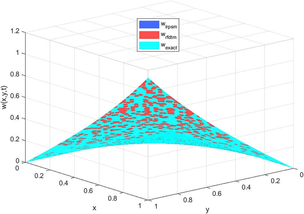
Example 1: RFDTM vs LTRPSM vs exact solution:
6.1.2 Solution by LTRPSM
We solved the same problem with Laplace-transformed power series method. Applying the Laplace transformation on both sides of Eq. (16) and rearranging the terms and using the preliminary criteria, we obtain
The kth LTR function can be defined as
Let the kth curtailed solution of (19) be
Substituting
Using
we obtain
Substituting
into Eq. (20), and applying
we obtain
in Eq. (20), and applying
we obtain
Taking inverse LT on both sides, we obtain the estimated solution as
6.2 Non-linear TFTE
Consider the two-dimensional non-linear TFTE
in compliance with
6.2.1 Solution by RFDTM
Applying the RFDT on both sides of the given Eq. (23), the following recurrence relation is obtained:
where
Using the initial constraints, the estimated solution is obtained as follows:
The results can be compared for
6.2.2 Solution by LTRPSM
Taking the LT on both sides of Eq. (23), using the preliminary criteria and with rearrangement of terms, we can write
The kth curtailed LTR can be written as
Let the kth curtailed solution of (26) be
Substituting
Using
we obtain
Substituting
Then,
implies
Substituting
Then, by
and using the Caputo fractional version of the L’Hopital’s rule as described in Kassim and Tatar [44], we obtain
Thus, the third curtailed solution becomes
On taking the inverse LT, the solution of the original telegraph Eq. (23) can be given as
where
7 Results and discussion
In this article, we tried calculating an estimated series solution of a linear and a non-linear TFTE by RFDTM (18, 25) and LTRPSM (22, 32).
The two methods can be considered semi analytic in nature and they give a series solution that has to be curtailed. More the term count in the series solution, better is the estimation, but here we restricted our solution for four terms only. Since it is difficult to find the closed-form solution of FDE, we compared the available closed-form solution for
For the linear TFTE (16), a pictorial comparison is made in the two methods in Figures 1–4. It can be observed that the solutions by the two methods completely overlap for
For the non-linear TFTE (23), a pictorial comparison is made in the two methods in Figures 8, 9, 10, 11. It can be observed that the solution by the two methods overlaps only for

Example 2: RFDTM vs LTRPSM:

Example 2: RFDTM vs LTRPSM:

Example 2: RFDTM vs LTRPSM:

Example 2: RFDTM vs LTRPSM:

Example 2: RFDTM vs LTRPSM vs exact solution:

Example 2: RFDTM vs LTRPSM vs exact solution:

Example 2: RFDTM vs LTRPSM vs exact solution:
8 Conclusion
To sum up, this work explores the solution of the fractional form of telegraph equation, which is a benchmark model for the physical behaviors exhibiting dual nature (wave propagation + diffusion). We solved the TFTE with two popular methods RFDTM and LTRPSM, which give a series solution. By taking only a small number of terms (here four) in the series solution, the results of both methods are found to be same for
Thus, we conclude that the RFDTM provides better solutions for linear as well as non-linear TFTE as compared to the LTRPSM. In addition to that, we must admit that the unavailability of the exact solutions of the FDEs is a major limitation for our work; however, it is also the driving force for the researchers to explore and develop analytic, semi-analytic, and numerical methods that may produce best approximate solutions. Another aspect to be worked upon is to understand why the solution of the non-linear system when solved with RFDTM is close to the exact solution for small values of
This work can further be extended by incorporating other definitions of fractional derivatives and by applying other transforms. This work can be extended to solve the space-fractional telegraph equation as well as the space-time-fractional analog of the equation. The methods addressed in this work or their modified versions can be applied to solve propagation and diffusion-related problems in engineering and sciences.
Acknowledgments
The authors would like to acknowledge the anonymous reviewers for their valuable suggestions.
-
Funding information: Authors state no funding involved.
-
Author contributions: All authors have accepted responsibility for the entire content of this manuscript and approved its submission.
-
Conflict of interest: The authors state no conflict of interest.
-
Data availability statement: Data sharing is not applicable to this article as no datasets were generated or analysed during the current study.
References
[1] Thomson III W. On the theory of the electric telegraph. Proc R Soc Lond. 1856;31(7):382–99. 10.1098/rspl.1854.0093Search in Google Scholar
[2] Debnath L. Linear partial differential equations. In: Nonlinear partial differential equations for scientists and engineers. Boston: Birkhäuser; 2012. p. 1–47. 10.1007/978-0-8176-8265-1_1Search in Google Scholar
[3] Metaxas AA, Meredith RJ. Industrial microwave heating. United Kingdom: IET; 1983. Search in Google Scholar
[4] Jordan PM, Puri A. Digital signal propagation in dispersive media. J Appl Phys. 1999;85(3):1273–82. 10.1063/1.369258Search in Google Scholar
[5] Ōkubo A. Application of the telegraph equation to oceanic diffusion: another mathematical model. Vol. 71. No. 3. Chesapeake Bay Institute, Johns Hopkins University. 1971; Search in Google Scholar
[6] Holmes EE. Are diffusion models too simple? A comparison with telegraph models of invasion. Am Nat. 1993;142(5):779–95. 10.1086/285572Search in Google Scholar PubMed
[7] Banasiak J, Mika JR. Singularly perturbed telegraph equations with applications in the random walk theory. Int J Stoch Anal. 1998;11:9–28. 10.1155/S1048953398000021Search in Google Scholar
[8] Khan D, Ali G, Kumam P, Almusawa MY, Galal AM. Time fractional model of free convection flow and dusty two-phase couple stress fluid along vertical plates. ZAMM J Appl Math Mech. 2023;103(5):e202200369. 10.1002/zamm.202200369Search in Google Scholar
[9] Khan D, Ali G, Kumam P, Suttiarporn P. A generalized electro-osmotic MHD flow of hybrid ferrofluid through Fourier and Fickas law in inclined microchannel. Numer Heat Transf Part A Appl. 2024;85(18):3091–109. 10.1080/10407782.2023.2232535Search in Google Scholar
[10] Jan R, Razak NNA, Boulaaras S, Rehman ZU, Bahramand S. Mathematical analysis of the transmission dynamics of viral infection with effective control policies via fractional derivative. Nonlinear Eng. 2023;12(1):20220342. 10.1515/nleng-2022-0342Search in Google Scholar
[11] Jan R, Boulaaras S, Alyobi S, Rajagopal K, Jawad M. Fractional dynamics of the transmission phenomena of dengue infection with vaccination. Discrete Contin Dyn Syst- S. 2023;16(8):2096–117. 10.3934/dcdss.2022154Search in Google Scholar
[12] Sikora B. Remarks on the Caputo fractional derivative. Minut. 2023;5:76–84. Search in Google Scholar
[13] Rehman ZU, Boulaaras S, Jan R, Ahmad I, Bahramand S. Computational analysis of financial system through non-integer derivative. J Comput Sci. 2024;75:102204. 10.1016/j.jocs.2023.102204Search in Google Scholar
[14] Kumar D, Singh J, Kumar S. Analytic and approximate solutions of space-time fractional telegraph equations via Laplace transform. Walailak J Sci Technol. 2014;11(8):711–28. Search in Google Scholar
[15] Momani S. Analytic and approximate solutions of the space-and time-fractional telegraph equations. Appl Math Comput. 2005;170(2):1126–34. 10.1016/j.amc.2005.01.009Search in Google Scholar
[16] Boyadjiev L, Luchko Y. The neutral-fractional telegraph equation. Math Model Nat Phenom. 2017;12(6):51–67. 10.1051/mmnp/2017064Search in Google Scholar
[17] Dehghan M, Salehi R. A method based on meshless approach for the numerical solution of the two-space dimensional hyperbolic telegraph equation. Math Methods Appl Sci. 2012;35(10):1220–33. 10.1002/mma.2517Search in Google Scholar
[18] Srivastava VK, Awasthi MK, Chaurasia RK. Reduced differential transform method to solve two and three dimensional second order hyperbolic telegraph equations. J King Saud Univ Eng Sci. 2017;29(2):166–71. 10.1016/j.jksues.2014.04.010Search in Google Scholar
[19] Khan H, Shah R, Kumam P, Baleanu D, Arif M. An efficient analytical technique, for the solution of fractional-order telegraph equations. Mathematics. 2019;7(5):426. 10.3390/math7050426Search in Google Scholar
[20] Khan H, Shah R, Baleanu D, Kumam P, Arif M. Analytical solution of fractional-order hyperbolic telegraph equation, using natural transform decomposition method. Electronics. 2019;8(9):1015. 10.3390/electronics8091015Search in Google Scholar
[21] Hamza AE, Mohamed MZ, Abd Elmohmoud EM, Magzoub M. Conformable Sumudu transform of space-time fractional telegraph equation. Abstr Appl Anal. 2021;2021(1):6682994. 10.1155/2021/6682994Search in Google Scholar
[22] Kapoor M, Shah NA, Saleem S, Weera W. An analytical approach for fractional hyperbolic telegraph equation using Shehu transform in one, two and three dimensions. Mathematics. 2022;10(12):1961. 10.3390/math10121961Search in Google Scholar
[23] Arora G, Pant R, Emadifar H, Khademi M. Numerical solution of fractional relaxation-oscillation equation by using residual power series method. Alex Eng J. 2023;73:249–57. 10.1016/j.aej.2023.04.055Search in Google Scholar
[24] Al-Smadi M. Solving initial value problems by residual power series method. Theor Math Appl. 2013;3(1):199–210. Search in Google Scholar
[25] Zhang J, Wei Z, Li L, Zhou C. Least-squares residual power series method for the time-fractional differential equations. Complexity. 2019;2019(1):6159024. 10.1155/2019/6159024Search in Google Scholar
[26] Dawar A, Khan H, Islam S, Khan W. The improved residual power series method for a system of differential equations: a new semi-numerical method. Int J Model Simul. 2023;1–14. 10.1080/02286203.2023.2270884.Search in Google Scholar
[27] Alquran M. Analytical solutions of fractional foam drainage equation by residual power series method. Math Sci. 2014;8(4):153–60. 10.1007/s40096-015-0141-1Search in Google Scholar
[28] Khresat H, El-Ajou A, Al-Omari S, Alhazmi SE, Oqielat MA. Exact and approximate solutions for linear and non-linear partial differential equations via Laplace residual power series method. Axioms. 2023;12(7):694. 10.3390/axioms12070694Search in Google Scholar
[29] Alaroud M. Application of Laplace residual power series method for approximate solutions of fractional IVP’s. Alex Eng J. 2022;61(2):1585–95. 10.1016/j.aej.2021.06.065Search in Google Scholar
[30] Pant R, Arora G, Singh BK, Emadifar H. Numerical solution of two-dimensional fractional differential equations using Laplace transform with residual power series method. Nonlinear Eng. 2024;13(1):20220347. 10.1515/nleng-2022-0347Search in Google Scholar
[31] Keskin Y, Oturanc G. Reduced differential transform method for partial differential equations. Int J Nonlinear SciNumer Simul. 2009;10(6):741–50. 10.1515/IJNSNS.2009.10.6.741Search in Google Scholar
[32] Wang KL, Wang KJ. A modification of the reduced differential transform method for fractional calculus. Therm Sci. 2018;22(4):1871–5. 10.2298/TSCI1804871WSearch in Google Scholar
[33] Patel HS, Patel T. Applications of fractional reduced differential transform method for solving the generalized fractional-order Fitzhugh-Nagumo equation. Int J Appl Comput Math. 2021;7(5):188. 10.1007/s40819-021-01130-2Search in Google Scholar
[34] Saeed U, Umair M. A modified method for solving non-linear time and space fractional partial differential equations. Eng Comput. 2019;36(7):2162–78. 10.1108/EC-01-2019-0011Search in Google Scholar
[35] Rashid S, Ashraf R, Hammouch Z. New generalized fuzzy transform computations for solving fractional partial differential equations arising in oceanography. J Ocean Eng Sci. 2023;8(1):55–78. 10.1016/j.joes.2021.11.004Search in Google Scholar
[36] Saifullah S, Ali A, Khan A, Shah K, Abdeljawad T. A novel tempered fractional transform: Theory, properties and applications to differential equations. Fractals. 2023;31(10):2340045. 10.1142/S0218348X23400455Search in Google Scholar
[37] Chu YM, Jneid M, Chaouk A, Inc M, Rezazadeh H, Houwe A. Local time fractional reduced differential transform method for solving local time fractional telegraph equations. Fractals. 2024;32(4):2340128. 10.1142/S0218348X2340128XSearch in Google Scholar
[38] Podlubny I. Fractional differential equations: an introduction to fractional derivatives, fractional differential equations, to methods of their solution and some of their applications. San Diego: Academic Press; 1999. vol. 198. Search in Google Scholar
[39] Miller KS, Ross B. An introduction to the fractional calculus and fractional differential equations. New York: Wiley; 1993. Search in Google Scholar
[40] Arora G, Pratiksha. A cumulative study on differential transform method. Int J Math Eng Manag Sci. 2019;4(1):170. 10.33889/IJMEMS.2019.4.1-015Search in Google Scholar
[41] Srivastava VK, Mishra N, Kumar S, Singh BK, Awasthi MK. Reduced differential transform method for solving (1+n)-Dimensional Burgers’ equation. Egypt J Basic Appl Sci. 2014;1(2):115–9. 10.1016/j.ejbas.2014.05.001Search in Google Scholar
[42] Ünal E, Gökdoğan A. Solution of conformable fractional ordinary differential equations via differential transform method. Optik. 2017;128:264–73. 10.1016/j.ijleo.2016.10.031Search in Google Scholar
[43] Abuasad S, Hashim I, Abdul Karim SA. Modified fractional reduced differential transform method for the solution of multiterm time-fractional diffusion equations. Adv Math Phys. 2019;2019(1):5703916. 10.1155/2019/5703916Search in Google Scholar
[44] Kassim MD, Tatar NE. Asymptotic Behavior for Fractional Systems with Lower-Order Fractional Derivatives. Prog Fract Differ Appl. 2023;9(1):145–66. 10.18576/pfda/090111Search in Google Scholar
© 2025 the author(s), published by De Gruyter
This work is licensed under the Creative Commons Attribution 4.0 International License.
Articles in the same Issue
- Research Articles
- Generalized (ψ,φ)-contraction to investigate Volterra integral inclusions and fractal fractional PDEs in super-metric space with numerical experiments
- Solitons in ultrasound imaging: Exploring applications and enhancements via the Westervelt equation
- Stochastic improved Simpson for solving nonlinear fractional-order systems using product integration rules
- Exploring dynamical features like bifurcation assessment, sensitivity visualization, and solitary wave solutions of the integrable Akbota equation
- Research on surface defect detection method and optimization of paper-plastic composite bag based on improved combined segmentation algorithm
- Impact the sulphur content in Iraqi crude oil on the mechanical properties and corrosion behaviour of carbon steel in various types of API 5L pipelines and ASTM 106 grade B
- Unravelling quiescent optical solitons: An exploration of the complex Ginzburg–Landau equation with nonlinear chromatic dispersion and self-phase modulation
- Perturbation-iteration approach for fractional-order logistic differential equations
- Variational formulations for the Euler and Navier–Stokes systems in fluid mechanics and related models
- Rotor response to unbalanced load and system performance considering variable bearing profile
- DeepFowl: Disease prediction from chicken excreta images using deep learning
- Channel flow of Ellis fluid due to cilia motion
- A case study of fractional-order varicella virus model to nonlinear dynamics strategy for control and prevalence
- Multi-point estimation weldment recognition and estimation of pose with data-driven robotics design
- Analysis of Hall current and nonuniform heating effects on magneto-convection between vertically aligned plates under the influence of electric and magnetic fields
- A comparative study on residual power series method and differential transform method through the time-fractional telegraph equation
- Insights from the nonlinear Schrödinger–Hirota equation with chromatic dispersion: Dynamics in fiber–optic communication
- Mathematical analysis of Jeffrey ferrofluid on stretching surface with the Darcy–Forchheimer model
- Exploring the interaction between lump, stripe and double-stripe, and periodic wave solutions of the Konopelchenko–Dubrovsky–Kaup–Kupershmidt system
- Computational investigation of tuberculosis and HIV/AIDS co-infection in fuzzy environment
- Signature verification by geometry and image processing
- Theoretical and numerical approach for quantifying sensitivity to system parameters of nonlinear systems
- Chaotic behaviors, stability, and solitary wave propagations of M-fractional LWE equation in magneto-electro-elastic circular rod
- Dynamic analysis and optimization of syphilis spread: Simulations, integrating treatment and public health interventions
- Visco-thermoelastic rectangular plate under uniform loading: A study of deflection
- Threshold dynamics and optimal control of an epidemiological smoking model
- Numerical computational model for an unsteady hybrid nanofluid flow in a porous medium past an MHD rotating sheet
- Regression prediction model of fabric brightness based on light and shadow reconstruction of layered images
- Dynamics and prevention of gemini virus infection in red chili crops studied with generalized fractional operator: Analysis and modeling
- Qualitative analysis on existence and stability of nonlinear fractional dynamic equations on time scales
- Fractional-order super-twisting sliding mode active disturbance rejection control for electro-hydraulic position servo systems
- Analytical exploration and parametric insights into optical solitons in magneto-optic waveguides: Advances in nonlinear dynamics for applied sciences
- Bifurcation dynamics and optical soliton structures in the nonlinear Schrödinger–Bopp–Podolsky system
- User profiling in university libraries by combining multi-perspective clustering algorithm and reader behavior analysis
- Exploring bifurcation and chaos control in a discrete-time Lotka–Volterra model framework for COVID-19 modeling
- Review Article
- Haar wavelet collocation method for existence and numerical solutions of fourth-order integro-differential equations with bounded coefficients
- Special Issue: Nonlinear Analysis and Design of Communication Networks for IoT Applications - Part II
- Silicon-based all-optical wavelength converter for on-chip optical interconnection
- Research on a path-tracking control system of unmanned rollers based on an optimization algorithm and real-time feedback
- Analysis of the sports action recognition model based on the LSTM recurrent neural network
- Industrial robot trajectory error compensation based on enhanced transfer convolutional neural networks
- Research on IoT network performance prediction model of power grid warehouse based on nonlinear GA-BP neural network
- Interactive recommendation of social network communication between cities based on GNN and user preferences
- Application of improved P-BEM in time varying channel prediction in 5G high-speed mobile communication system
- Construction of a BIM smart building collaborative design model combining the Internet of Things
- Optimizing malicious website prediction: An advanced XGBoost-based machine learning model
- Economic operation analysis of the power grid combining communication network and distributed optimization algorithm
- Sports video temporal action detection technology based on an improved MSST algorithm
- Internet of things data security and privacy protection based on improved federated learning
- Enterprise power emission reduction technology based on the LSTM–SVM model
- Construction of multi-style face models based on artistic image generation algorithms
- Research and application of interactive digital twin monitoring system for photovoltaic power station based on global perception
- Special Issue: Decision and Control in Nonlinear Systems - Part II
- Animation video frame prediction based on ConvGRU fine-grained synthesis flow
- Application of GGNN inference propagation model for martial art intensity evaluation
- Benefit evaluation of building energy-saving renovation projects based on BWM weighting method
- Deep neural network application in real-time economic dispatch and frequency control of microgrids
- Real-time force/position control of soft growing robots: A data-driven model predictive approach
- Mechanical product design and manufacturing system based on CNN and server optimization algorithm
- Application of finite element analysis in the formal analysis of ancient architectural plaque section
- Research on territorial spatial planning based on data mining and geographic information visualization
- Fault diagnosis of agricultural sprinkler irrigation machinery equipment based on machine vision
- Closure technology of large span steel truss arch bridge with temporarily fixed edge supports
- Intelligent accounting question-answering robot based on a large language model and knowledge graph
- Analysis of manufacturing and retailer blockchain decision based on resource recyclability
- Flexible manufacturing workshop mechanical processing and product scheduling algorithm based on MES
- Exploration of indoor environment perception and design model based on virtual reality technology
- Tennis automatic ball-picking robot based on image object detection and positioning technology
- A new CNN deep learning model for computer-intelligent color matching
- Design of AR-based general computer technology experiment demonstration platform
- Indoor environment monitoring method based on the fusion of audio recognition and video patrol features
- Health condition prediction method of the computer numerical control machine tool parts by ensembling digital twins and improved LSTM networks
- Establishment of a green degree evaluation model for wall materials based on lifecycle
- Quantitative evaluation of college music teaching pronunciation based on nonlinear feature extraction
- Multi-index nonlinear robust virtual synchronous generator control method for microgrid inverters
- Manufacturing engineering production line scheduling management technology integrating availability constraints and heuristic rules
- Analysis of digital intelligent financial audit system based on improved BiLSTM neural network
- Attention community discovery model applied to complex network information analysis
- A neural collaborative filtering recommendation algorithm based on attention mechanism and contrastive learning
- Rehabilitation training method for motor dysfunction based on video stream matching
- Research on façade design for cold-region buildings based on artificial neural networks and parametric modeling techniques
- Intelligent implementation of muscle strain identification algorithm in Mi health exercise induced waist muscle strain
- Optimization design of urban rainwater and flood drainage system based on SWMM
- Improved GA for construction progress and cost management in construction projects
- Evaluation and prediction of SVM parameters in engineering cost based on random forest hybrid optimization
- Museum intelligent warning system based on wireless data module
- Optimization design and research of mechatronics based on torque motor control algorithm
- Special Issue: Nonlinear Engineering’s significance in Materials Science
- Experimental research on the degradation of chemical industrial wastewater by combined hydrodynamic cavitation based on nonlinear dynamic model
- Study on low-cycle fatigue life of nickel-based superalloy GH4586 at various temperatures
- Some results of solutions to neutral stochastic functional operator-differential equations
- Ultrasonic cavitation did not occur in high-pressure CO2 liquid
- Research on the performance of a novel type of cemented filler material for coal mine opening and filling
- Testing of recycled fine aggregate concrete’s mechanical properties using recycled fine aggregate concrete and research on technology for highway construction
- A modified fuzzy TOPSIS approach for the condition assessment of existing bridges
- Nonlinear structural and vibration analysis of straddle monorail pantograph under random excitations
- Achieving high efficiency and stability in blue OLEDs: Role of wide-gap hosts and emitter interactions
- Construction of teaching quality evaluation model of online dance teaching course based on improved PSO-BPNN
- Enhanced electrical conductivity and electromagnetic shielding properties of multi-component polymer/graphite nanocomposites prepared by solid-state shear milling
- Optimization of thermal characteristics of buried composite phase-change energy storage walls based on nonlinear engineering methods
- A higher-performance big data-based movie recommendation system
- Nonlinear impact of minimum wage on labor employment in China
- Nonlinear comprehensive evaluation method based on information entropy and discrimination optimization
- Application of numerical calculation methods in stability analysis of pile foundation under complex foundation conditions
- Research on the contribution of shale gas development and utilization in Sichuan Province to carbon peak based on the PSA process
- Characteristics of tight oil reservoirs and their impact on seepage flow from a nonlinear engineering perspective
- Nonlinear deformation decomposition and mode identification of plane structures via orthogonal theory
- Numerical simulation of damage mechanism in rock with cracks impacted by self-excited pulsed jet based on SPH-FEM coupling method: The perspective of nonlinear engineering and materials science
- Cross-scale modeling and collaborative optimization of ethanol-catalyzed coupling to produce C4 olefins: Nonlinear modeling and collaborative optimization strategies
- Unequal width T-node stress concentration factor analysis of stiffened rectangular steel pipe concrete
- Special Issue: Advances in Nonlinear Dynamics and Control
- Development of a cognitive blood glucose–insulin control strategy design for a nonlinear diabetic patient model
- Big data-based optimized model of building design in the context of rural revitalization
- Multi-UAV assisted air-to-ground data collection for ground sensors with unknown positions
- Design of urban and rural elderly care public areas integrating person-environment fit theory
- Application of lossless signal transmission technology in piano timbre recognition
- Application of improved GA in optimizing rural tourism routes
- Architectural animation generation system based on AL-GAN algorithm
- Advanced sentiment analysis in online shopping: Implementing LSTM models analyzing E-commerce user sentiments
- Intelligent recommendation algorithm for piano tracks based on the CNN model
- Visualization of large-scale user association feature data based on a nonlinear dimensionality reduction method
- Low-carbon economic optimization of microgrid clusters based on an energy interaction operation strategy
- Optimization effect of video data extraction and search based on Faster-RCNN hybrid model on intelligent information systems
- Construction of image segmentation system combining TC and swarm intelligence algorithm
- Particle swarm optimization and fuzzy C-means clustering algorithm for the adhesive layer defect detection
- Optimization of student learning status by instructional intervention decision-making techniques incorporating reinforcement learning
- Fuzzy model-based stabilization control and state estimation of nonlinear systems
- Optimization of distribution network scheduling based on BA and photovoltaic uncertainty
- Tai Chi movement segmentation and recognition on the grounds of multi-sensor data fusion and the DBSCAN algorithm
- Special Issue: Dynamic Engineering and Control Methods for the Nonlinear Systems - Part III
- Generalized numerical RKM method for solving sixth-order fractional partial differential equations