Mathematical analysis of Jeffrey ferrofluid on stretching surface with the Darcy–Forchheimer model
-
Musharafa Saleem
 und
Aun Haider
und
Aun Haider

Abstract
The study examines the laminar two-dimensional flow with heat and mass transfer of Jeffrey fluid having thermal radiation and heat source–sink effects past a linearly inclined vertical stretched sheet under Stefan blowing. The impact of a magnetic dipole is also examined on two different thermal processes: prescribed surface temperature (PST) and prescribed heat flux (PHF). Furthermore, the Darcy–Forchheimer model, mixed convection, Buongiorno fluid model, and slip conditions are incorporated to enhance these thermal and concentration characteristics. With their unique combination of liquid and magnetic properties, ferromagnetic fluids are useful in a variety of scientific and industrial fields. The purpose of this study is to investigate how viscous dissipation, Soret and Dufour effects, and a magnetic dipole affect fluid flow, heat transfer, and concentration transfers in Jeffrey fluid over an inclined vertical stretching surface. For the concentration profile, the rheological model (a system of partial differential equations) incorporates partial slip effects, thermophoresis, and Brownian motion effects. Using similarity transformations, the model equations are transformed into coupled nonlinear ordinary differential equations. The BVP4C method is employed to obtain solutions to the fluid’s velocity, temperature, and concentration profiles. Various parameters are analyzed to determine their influence, with effects represented in tables and graphs for both PST and PHF thermal processes. Results for specific cases are compared with previously published results, showing good agreement. Thermal radiation increases the temperature for PHF processes, while the magnetic dipole reduces the fluid’s velocity and increases the temperature for PST.
Nomenclature
-
-
stretching constant
-
-
skin friction coefficient
-
-
ambient concentration of nanoparticle
-
-
concentration of nanoparticles at surface
-
-
Brownian diffusion parameter
- Dr
-
Dufour number
-
-
thermophoresis diffusion parameter
- Fr
-
Darcy–Forchheimer parameter
-
-
velocity profile
-
-
dimensionless velocity stream function
- GC
-
Grashof number for concentration
- GT
-
Grashof number for temperature
-
-
magnetic field
-
-
thermal conductivity
-
-
magnetic parameter
- Nt
-
thermophoretic parameter
- Nb
-
Brownian parameter
- Nu
-
local Nusselt number
-
-
heat source–sink parameter
- Pr
-
Prandtl number
-
-
Reynolds number
-
-
thermal radiation parameter
- Sc
-
Schmidt number
- Sh
-
local Sherwood number
-
-
ambient temperature
-
-
reference temperature
-
-
Curie temperature
-
-
velocities
-
-
free stream velocity
-
-
velocity at the wall
-
Greeks
-
-
thermal diffusivity
-
-
magnetic field strength
-
-
ferromagnetic interaction parameter
-
-
dimensionless distance from the origin to the magnetic dipole
-
-
viscous dissipation parameter
-
-
dynamic viscosity
-
-
kinematic viscosity
-
-
slip parameter
-
-
dimensionless concentration function
-
-
stream function
-
-
concentration profile
-
-
density
-
-
dimensionless temperature
-
-
temperature profile
-
-
Curie temperature ratio
-
-
dimensionless similarity variable
-
Subscripts
-
-
conditions at the surface
-
-
conditions at the free stream
- 0
-
conditions at the reference surface
1 Introduction
Ferromagnetic fluids (FMFs), or ferrofluids, are liquids that become strongly magnetized when exposed to a magnetic field. These fluids are colloidal suspensions of nanoscale ferromagnetic, or ferrimagnetic particles (usually magnetite, hematite, or some other compound containing iron) suspended in a carrier fluid, typically water or an organic solvent. A surfactant coats the particles to prevent clumping and ensure even dispersion. This can be water, oil, or other suitable solvents that allow the suspension to remain stable. When exposed to a magnetic field, the nanoparticles align along the magnetic field lines, causing the fluid to exhibit magnetic properties. Magnetic fluids [1,2] consist of super-paramagnetic, ferromagnetic, or non-magnetic carrier liquid particles suspended in an organic solvent. FMFs typically comprise nanometer-sized particles, while magneto-rheological fluids contain micrometer-sized particles. The fluid can change its shape and behavior under the influence of a magnetic field. It is used in rotary seals on computer hard drives to keep dust and other particles out while allowing the spindle to rotate. It has potential applications in drug delivery and magnetic resonance imaging (MRI). It is used in loudspeakers to dampen vibrations and improve sound quality, and in heat transfer applications. In the presence of a strong magnetic field, ferrofluids can form spike-like structures due to magnetic field lines, a phenomenon known as normal-field instability. They exhibit super-paramagnetic, meaning they have magnetic properties only in the presence of an external magnetic field and do not retain residual magnetism when the field is removed. The hydrodynamic, rheological, thermophysical, and magnetic properties of FMF are harnessed to develop sealers [3–5], heat-transfer devices [6], dampers [7], as well as inclination angle and pressure sensors [8,9]. To date, numerous studies have explored the potential applications of FMFs in medicine, such as drug delivery [10–12], magnetic hyperthermia, and as a difference medium for medical diagnostics, including MRI [13,14].
Andersson and Valnes [15] examined the flow of FMFs carried out on a flat sheet influenced by a magnetic dipole system. FMFs play a crucial role in various electrochemical, mechanical, and electrical devices, such as computer hard disk seals, lithographic designs, and rotating rods and shafts [16,17]. Zeeshan et al. [18] considered the possession of a magnetic dipole on the radiative flow of viscous FMFs over an elastic sheet. Sohail et al. [19] analyzed the manipulation of FMFs in the context of magnetic drug targeting. Kumar et al. [20] studied the impact of a magnetic dipole on the flow of FMF above extending surface. Almaneea [21] discussed the thermal characteristics of FMFs with hybrid nano-metallic structures in a Forchheimer absorbent medium under the impact of a magnetic dipole. Gowda et al. [22] investigated the influence of Stefan blowing and magnetic dipole effects on the flow of FMFs over a stretching sheet. They solved the resulting equations using the Runge–Kutta–Fehlberg 45 method in combination with the shooting technique. Hussain et al. [23] examined the properties of magnetic dipole contributions to the radiative flow of FMFs, considering the aspects of viscous dissipation.
On the other hand, considering non-Newtonian fluids is of significant real-world importance, it requires mathematical imagination to report the highly non-linear partial differential equations involved. Nowadays, it is understood that fluids generally exhibit viscoelastic behavior under stress. Consequently, both industrial and biological fluids are predictable as non-Newtonian. Many studies have been conducted to explore the effects of relevant parameters in non-Newtonian models, especially on the incidence of a magnetic dipole. Zeeshan and Majeed [24], for instance, examined the heat transfer breakdown of Jeffrey fluid flow over a stretching sheet with suction/injection and the influence of a magnetic dipole. The Jeffrey fluid is of interest due to its linear viscoelastic properties, prompting the exploration of nonlinear viscoelastic fluids. Qualitative and quantitative approaches to Hartmann boundary layer (BL) peristaltic flow of Jeffrey fluid have been performed by Yasmeen et al. [25]. The boundary value problem (BVP) is explained systematically by means of a remarkable perturbation method together with a higher-order identical technique. They discussed the problem of large magnetic fields using both an applied and theoretical point of view. In a study conducted by Abbas et al. [26], Jeffrey fluid was considered under Soret and Dufour and stretched over a curved Riga surface. They reported that the velocity function becomes smaller due to improved values of the modified Hartmann number. Ashraf et al. [27] discussed horizontal Jeffrey fluid film flow in
Recent advancements in engineering and geophysical methods have provided new insights into fluid movement inside absorbent materials. These approaches are applied in various fields, including grain preservation, groundwater management, porous bearing systems, air refinement in filtration systems, blood movement in lungs or arteries, and transport through permeable tubes. Scientists and engineers from multiple fields have shown a solid curiosity with these applications. A study on absorbent media frequently trusts on Darcy’s supposition [31], which is applicable only for small velocities with low permeability. However, many practical scenarios feature irregular porosity disseminations and improved movement rates, where Darcy’s theory fails to accurately represent the physical singularities. To address this limitation, non-Darcian possessions are incorporated to more precisely represent the actual behavior of the system. Forchheimer [32] reported for these possessions by accumulation a term that comprises the square of the velocity to the Darcian rate equation. Al-arabi et al. [33] investigated the Darcy–Forchheimer model and electromagnetic effects over a rotating cone and an expandable disk moving surface in a thermally hybrid nanofluid flow. Prakash et al. [34] examined the dynamics of irreversibility and melting heat transfer of Casson fluid inside an absorbent medium using Darcy–Forchheimer law. Ramana et al. [35] conducted numerical imitations to study the influences of Darcy–Forchheimer and Hall currents on dissipative Newtonian liquid flow over a thinner surface. Furthermore, Salahuddin et al. [36] analyzed the Darcy–Forchheimer behavior of viscous dissipation on radially tangent hyperbolic fluid with activation energy.
When forced and natural convection processes happen concurrently, the phenomenon called mixed convection occurs in fluid flow. This phenomenon is widely applicable in areas such as heating and ventilation systems, food processing, electronics cooling, solar collectors, glass production, building ventilation, furnaces, chemical reactors, and vehicle cooling. Yang and Du [37] have provided an extensive assessment of forced, free, and mixed convection phenomena in various fluids with different geometries. Current research is focused on investigating mixed convection with heat transfer procedures in composite symmetrical shapes, taking into account factors such as magnetohydrodynamics (MHD), porous media, flow control variables, and the use of nanofluids/hybrid nanofluids [38–40]. Another crucial area of study is the generation of irreversibility, which is vital for optimizing heat transfer efficiency. Many revisions have discovered mixed convection phenomena in variously shaped geometries beneath different thermal gradients and external or sliding wall motions [41–43]. Additionally, numerous scholars have examined hydrothermal phenomena in a range of multiphysical scenarios [44–46].
While linear thermal radiation is further common in many unremarkable applications, nonlinear thermal radiation plays a crucial role in certain situations somewhere a more accurate illustration of radiative heat transfer is necessary. Furthermore, studies have explored the utilization of nonlinear radiation. Thermal radiation is a type of electromagnetic radiation unconstrained by a material outstanding to the heat it produces, and its properties are determined by the material’s temperature. In previous studies [47,48], the stability analysis and the impact of thermal and concentration slip on hybrid Casson–Maxwell nanofluid over a stretched sheet affected by thermal radiation were addressed. Yedhiri et al. [49] investigated the time-dependent mixed convective MHD flow over an infinite vertical plate with thermal absorption. They observed that fluid velocity and temperature increase with rising radiation absorption factor, while temperature tends to reduction as thermal radiation increases. Rao and Deka [50] provided a numerical analysis of hybrid nanofluid utilizing thermal radiation in porous media. Madhu et al. [51] discussed the impacts of quadratic thermal radiation on oblique stagnation points across a cylinder in hybrid nanofluid flow. Alamirew and Awgichew [52] examined the nonlinear radiation effects on the mixed convective flow of Casson nanofluid past a vertically extending surface. Jiann et al. [53] studied the quadratic radiation impacts of melting phenomena on Carreau fluid flow about a stretchable cylinder.
Heat and mass transfer receive considerable influence from the Soret and Dufour effects during non-Newtonian fluid flows under conditions of thermal and concentration gradients. Researchers describe the Soret effect when species diffuse because of thermal gradients and the Dufour effect applies when chemical gradients produce thermal transport. The Soret and Dufour effects matter in three main application areas, including stretched surface flows porous media and MHD systems, because they combine thermal and mass diffusion behavior. Chemical reactions modify the effects through changes to concentration and temperature fields when present. The Soret effect receives reinforcement from exothermic reactions since these reactions elevate temperature gradients but endothermic reactions minimize heat availability, which impacts Dufour-driven heat transfer. The nonlinear interactions present between these components require proper examination during research involving nanofluids as well as biomedical flows and industrial cooling systems. The boundary conditions imposed on the system also have a strong impact on these transport phenomena. Placing the boundary under prescribed surface temperature (PST) control creates a constant temperature environment that directly controls both thermal diffusion and Soret influences. The Dufour effect receives influence from the thermal energy dedicated to diffusion through a process called prescribed heat flux (PHF). The choice of boundary conditions will either increase or decrease heat and mass transfer when implemented during chemical reactions. MHD flows through porous media experience substantial temperature variations when heat flux is prescribed at the boundary because reaction kinetics and mass transport patterns change resulting from these temperature changes. The interactions play vital roles in various applications that include polymer manufacturing alongside peristaltic operation in biological structures and energy system thermal management. Hussain et al. [54] studied the pseudo-plastic properties flow of a nanofluid with about a tall vertical cylinder, focusing on the interaction between thermophoresis and Brownian motion. Shafey et al. [55] conducted a theoretical analysis of the impact of these phenomena on the flow of Newtonian fluid past a nonlinearly stretching cylinder. Tawade et al. [56] inspected the effects of thermophoresis and Brownian motion on the flow of Casson nanofluid over a linearly stretching sheet. Sarfraz et al. [57] researched nanofluid flow and thermal energy transfer in the stagnation area involving the radial impingement of a rotating spherical cylinder. Jawad and Ghazwani [58] analyzed thermophoresis and Brownian motion in MHD flow over a cylinder secure with a porous medium. Sharma et al. [59] inspected the significance of these phenomena on the flow of water carrying Fe3O4 and Mn–ZnFe2O4 nanoparticles over a revolving disk. In a study conducted by Khan et al. [60], the unsteady MHD slip flow of a ternary hybrid Casson fluid through a nonlinear stretching disk embedded in a porous medium was analyzed, highlighting the significant role of slip conditions in heat transfer characteristics. Similarly, Khan et al. [61] explored the heat and mass transfer effects for the MHD flow of a Brinkman-type dusty fluid between fluctuating parallel vertical plates, considering arbitrary wall shear stress. Khan et al. [62] employed Laplace and Sumudu transforms to analyze the unsteady rotating MHD flow of second-grade hybrid nanofluids passing through porous media, thereby studying fluid behavior under these conditions. According to Khan et al. [63], the application of Poincaré–Lighthill perturbation analysis revealed how boundary conditions relating to Newtonian heating generate substantial effects on the temperature distribution of such dusty two-phase fluctuating flow. Khan et al. [64] developed a generalized analysis of electroosmotic MHD flow for hybrid ferrofluids inside an inclined microchannel through models based on Fourier and Fick laws. They showed the predictive power of fractional-order derivatives using a time-fractional model to examine the free convection of vertical plates carrying a dusty two-phase couple stress fluid [65]. The research conducted by Khan et al. [66] showed that heat transfer enhancements occur in MHD Falkner–Skan flow between parallel plates through the analysis of thermal radiation together with free convection and dusty fluid effects; the research demonstrated that thermal BL thickness changes significantly because of radiation. The research of Chen [67] established fundamental knowledge about how stretching surfaces affect buoyancy and external flow during laminar mixed convection. The researchers of Abel et al. [68] investigated viscoelastic MHD flow combined with heat transfer features across stretching sheets while studying viscous and Ohmic dissipations to reveal that these dissipation effects modify the thermal BL features. The research of Agarwal et al. [69] explored the Jeffrey slip fluid flow with magnetic dipole effect over a melting or permeable stretching sheet and demonstrated that slip operation modifies both velocity and temperature distributions.
The objectives of this study are as follows:
Investigate the continuous two-dimensional flow and heat transfer of Jeffrey fluid over a linearly inclined vertical stretched sheet.
Analyze the effects of thermal radiation and heat source–sink effects on the flow and heat transfer.
Examine the impact of a magnetic dipole on the flow and heat transfer processes.
Compare two different thermal processes: PST and PHF, and their effects on flow and heat transfer.
Explore the influence of viscous dissipation, Soret and Dufour effects, and magnetic dipole on the flow and heat transfer characteristics.
Enhance the rheological model by incorporating additional effects such as thermophoresis, Brownian motion, and activation energy to improve concentration profile predictions.
Transform model equations into coupled nonlinear ordinary differential equations (ODEs) using similarity transformations for numerical solution.
Utilize the BVP4C method to obtain solutions for fluid velocity and temperature profiles.
Analyze various parameters to determine their influence on the flow and heat transfer processes.
Present results through tables and graphs, comparing specific cases with previously published results to validate the model.
Investigate the specific impact of thermal radiation and magnetic dipole on fluid velocity and temperature profiles for both PST and PHF thermal processes.
2 Mathematical modeling
2.1 Flow assumptions
The key aims of this study are as follows:
1. Investigate flow with Darcy–Forchheimer effects and heat transfer:
To analyze the continuous two-dimensional flow with Darcy–Forchheimer effects and heat transfer characteristics of Jeffrey fluid over a linearly inclined vertical stretched sheet.
2. Examine thermal radiation and heat source–sink effects:
To understand the impact of thermal radiation and heat source–sink effects under different suction/injection conditions.
3. Explore the influence of magnetic dipole:
To determine the effects of a magnetic dipole on the flow and heat transfer for two thermal processes: PST and PHF.
4. Understand mixed convection:
To study the BL flow and heat transfer with mixed convection, essential for various industrial applications.
5. Assess viscous dissipation, Soret and Dufour effects:
To establish the impact of viscous dissipation, Soret and Dufour effects on the flow and heat transfer characteristics.
6. Enhance rheological model:
To enhance the Jeffrey fluid model by incorporating thermophoresis, Brownian motion, and activation energy effects, thereby improving the concentration profile.
7. Transform and solve model equations:
To transform the model equations into coupled nonlinear ODEs using similarity transformations and solve them using the BVP4C method.
8. Analyze the effects of various parameters:
To study how different parameters affect the flow and heat transfer, presenting these effects through tables and graphs for both PST and PHF conditions.
9. Compare with previous results:
To compare the results of specific cases with previously published results to validate the findings and ensure consistency.
10. Determine thermal radiation and magnetic dipole effects:
To determine that thermal radiation increases the temperature for both PST and PHF processes, and to study how the magnetic dipole influences the fluid’s velocity and temperature differently for PST and PHF processes.
2.2 Flow modeling
An electrically nonconducting, steady, and incompressible two-dimensional Jeffrey FMF flows over an inclined vertical linearly stretching sheet (Figure 1). The sheet stretches with a velocity

Schematic of two-dimensional Jaffery ferrofluid flow with inclined vertical stretched surface.
The Jeffrey model captures both viscous and elastic properties of the fluid. The parameters
When
When
The Jeffrey fluid model is used to describe the behavior of various complex fluids, such as polymer solutions, biological fluids, and other materials that exhibit both viscous and elastic properties. It is particularly useful in applications where the fluid’s response to deformation involves time-dependent effects. The Jeffrey fluid model provides a more accurate description of certain non-Newtonian fluids compared to simpler models such as the Newtonian or purely viscous models. It can capture the time-dependent behavior of fluids, making it suitable for modeling processes where fluid memory effects are significant. In summary, the Jeffrey fluid model is a versatile and useful tool in rheology for characterizing the behavior of complex fluids that exhibit both viscous and elastic properties, and it finds applications in various scientific and engineering fields. The governing BL equations for this Jeffrey ferrofluid system are expressed as follows [28,29]:
here,
The relevant boundary conditions take the following form [36,37]:
where
2.3 Magnetic dipole moment
The magnetic dipole moment [22,23] can influence the flow patterns and stability of the fluid, as the magnetic forces can either enhance or suppress turbulence depending on the configuration of the magnetic field and the properties of the fluid. In applications involving magnetic fluids or FMFs, the magnetic dipole moment of the particles affects their behavior in a flow. When subjected to an external magnetic field, these particles align along the field lines, which can alter the viscosity and flow characteristics of the fluid. The torque experienced by magnetic dipoles in a fluid can lead to rotational motions, which are significant in processes like mixing or in the design of magnetic stirrers. In summary, the magnetic dipole moment is a key parameter in understanding the interactions between magnetic fields and fluid flows, influencing both the dynamics of the fluids and the behavior of magnetic materials within them. The magnetic dipole generates a magnetic field that impacts the flow of the FMFs, which is represented mathematically by a magnetic scalar potential denoted as
where
Since the magnetic body force is generally proportional to the gradient of the magnitude of
By substituting Eqs (8) and (9) into Eq. (10) and expanding in powers of
The relationship between magnetization
where
2.4 Similarity transformations
Here, we define the dimensionless variables as follows:
where
2.5 Stream function
The stream function
Use the prime notation to denote differentiation with respect to
In order to obtain the solution for momentum equation, finally, we obtain the momentum equation as
Similarly, we will follow the same process for temperature and concentration. Now, the final BL equations in terms of ODEs are
Similarly,
with dimensionless boundary conditions
and the developing parameters are defined as
The aforementioned quantities can be defined as the Prandtl number, thermal radiation, ferromagnetic interaction parameter, Deborah number, viscous dissipation parameter, Grashof number for temperature, heat source–sink parameter, permeability parameter, Darcy–Forchheimer parameter, Grashof number for concentration, slip parameter, dimensionless distance from the origin to the magnetic dipole, Dufour number, Brownian motion parameter, Curie temperature ratio, and thermophoretic parameter.
3 Physical quantities
Skin friction, Nusselt number, and Sherwood number have significant applications across various engineering fields. Skin friction is crucial in aerospace, automotive, maritime, and pipeline engineering, where it helps minimize drag and optimize performance and fuel efficiency. The Nusselt number is vital in heat transfer analysis, which is used in the design of heat exchangers, cooling of electronic devices, heating, ventilation, and air conditioning systems, chemical processes, and solar collectors, ensuring effective thermal management. The Sherwood number plays a key role in mass transfer operations, aiding in the design of equipment for chemical engineering, environmental engineering, bioprocessing, food processing, and the pharmaceutical industry, optimizing processes such as drying, extraction, and pollutant dispersion. These dimensionless numbers help engineers characterize and improve the efficiency of various physical processes. In addition, the following categories have been established for the local expressions of skin friction coefficient
After using the similarity variables, the following dimensionless expressions are obtained as:
where
4 Results, discussion, and applications
4.1 Numerical technique
The results demonstrate the effective representation of the underlying physical principles governing the dynamics of momentum, heat, and concentration profiles using the employed numerical model. Moreover, these thermal and concentration characteristics are further enhanced by incorporating the Darcy–Forchheimer model, mixed convection, the Buongiorno fluid model, and slip conditions. This study holds the potential to contribute significantly to the advancement of engineering applications related to magnetic dipole moments. The findings are visually presented through plots and tables, aiding in a comprehensive understanding and comparison of the outcomes. Specifically, Figure 1 offers a graphical exploration of the considered assumptions within distinct flow transport scenarios, as outlined in Figure 2. This graphical analysis facilitates a clearer comprehension of the various factors at play in different flow conditions. The numerical solution for the given problem was implemented using MATLAB and the BVP4C method. The provided MATLAB code serves the purpose of generating graphs and exploring tabulated values for various physical parameters within this study. The mesh generation and error control mechanisms are dependent on the residuals obtained during the ongoing solution process. A relative error tolerance of

Graphical abstract.
Let us define the following functions as:
The set of equations are reduced to
with the transformed boundary conditions
4.2 Comparison
By comparing the numerical values of the Nusselt number for varying Prandtl numbers in Table 1, the accuracy of the modified approach is demonstrated. The table confirms the effectiveness of the improved method.
Comparison of the Nusselt number for different values of the Prandtl number (Pr), with all other parameters set to zero
| Pr |
|
|
|
Present values |
|---|---|---|---|---|
| 0.72 | 1.0885 | 1.088548 | 1.088527 | 1.0885252 |
| 1 | 1.3330 | 1.333333 | 1.333334 | 1.3333333 |
| 3 | 2.5097 | 2.5097134 | 2.509725 | 2.50977266 |
| 10 | 4.7968 | 4.796864 | 4.796873 | 4.796856998 |
4.3 Discussion
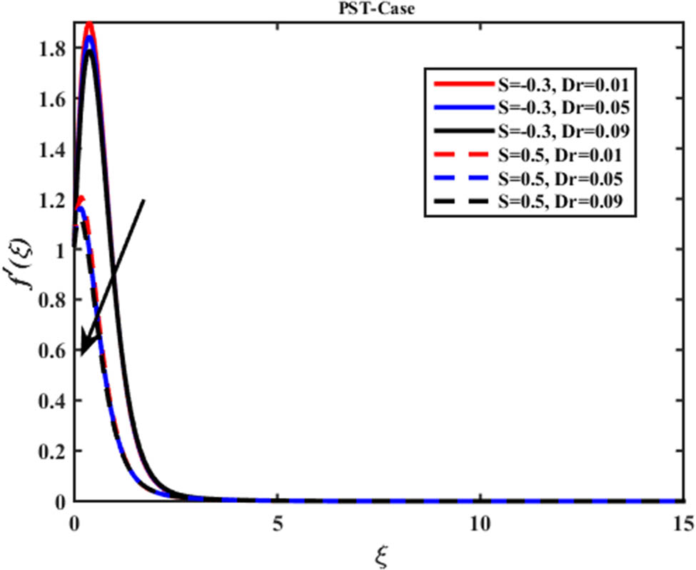
4.3.1 Velocity distribution on various pertinent parameters
This parameter

Interaction of suction and injection on Ferro–Jaffery fluid within the

Interaction of suction and injection on Ferro–Jaffery fluid within the

Interaction of suction and injection on Ferro–Jaffery fluid within the
Interaction of suction and injection on Ferro–Jaffery fluid within the Dr on velocity profile

Interaction of suction and injection on Ferro–Jaffery fluid within the Fr on velocity profile

Interaction of suction and injection on Ferro–Jaffery fluid within the

Interaction of suction and injection on Ferro–Jaffery fluid within the GC on velocityprofile

Interaction of suction and injection on Ferro–Jaffery fluid within the GT on velocity profile

Interaction of suction and injection on Ferro–Jaffery fluid within the

Interaction of suction and injection on Ferro–Jaffery fluid within the

Interaction of suction and injection on Ferro–Jaffery fluid within the
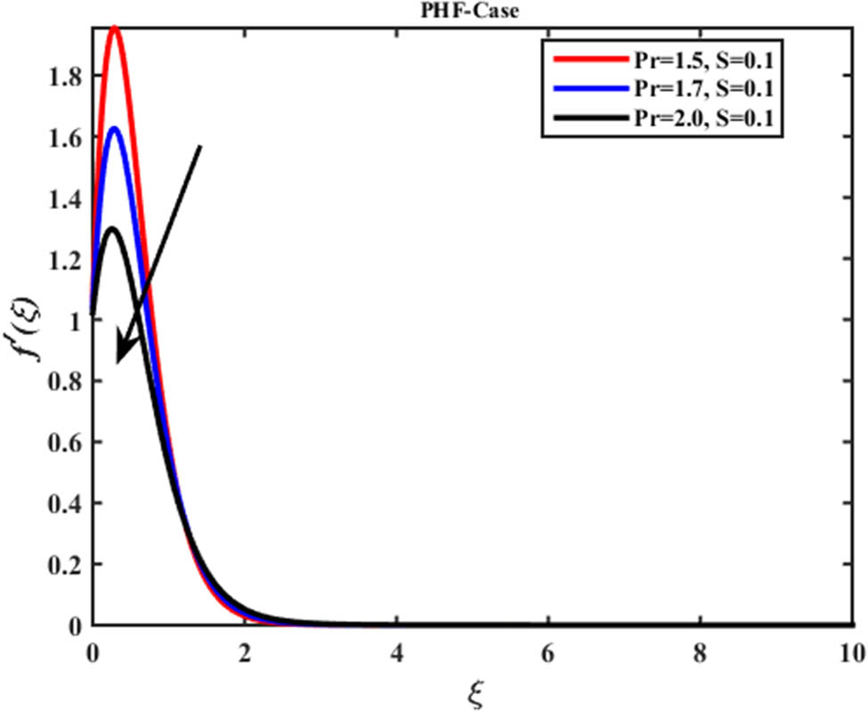
Interaction of suction and injection on Ferro–Jaffery fluid within the Pr on velocity profile

Interaction of suction and injection on Ferro–Jaffery fluid within the
4.3.2 Temperature distribution on various pertinent parameters
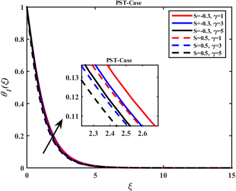
Figures 16, 17, 18, 19, 20, 21, 22, 23, 24, 25 are sketched to see the influences of important parameters on temperature velocity for PST/PHF cases in the occurrence of suction/injection. Here,

Interaction of suction and injection on Ferro–Jaffery fluid within the

Interaction of suction and injection on Ferro–Jaffery fluid within the GT on thermal profile
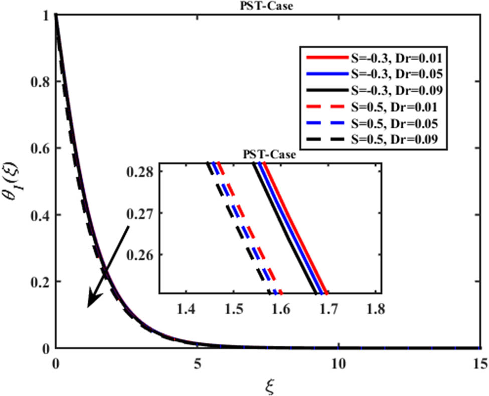
Interaction of suction and injection on Ferro–Jaffery fluid within the Dr on thermal profile
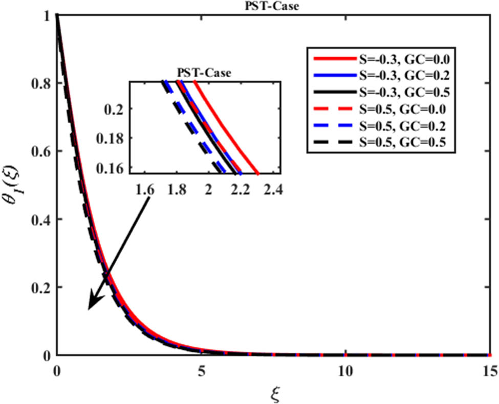
Interaction of suction and injection on Ferro–Jaffery fluid within the GC on thermal profile

Interaction of suction and injection on Ferro–Jaffery fluid within the Nt on thermal profile
Interaction of suction and injection on Ferro–Jaffery fluid within the
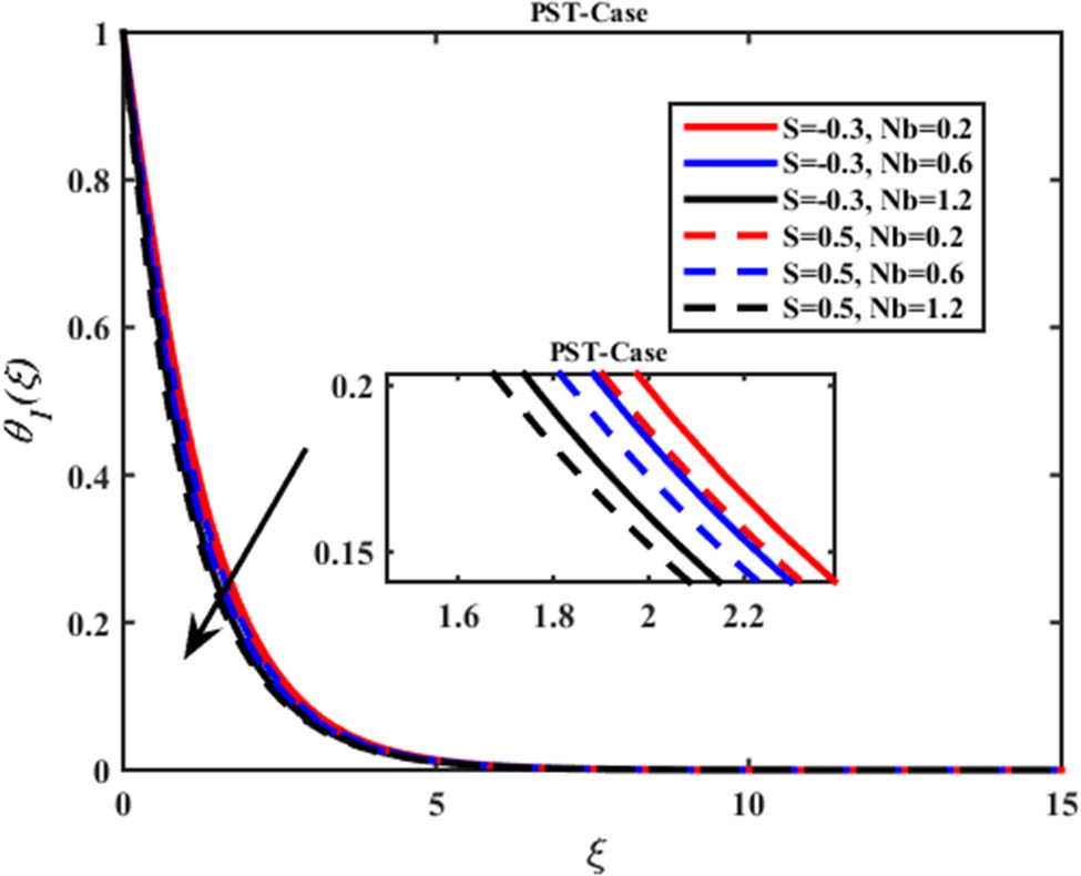
Interaction of suction and injection on Ferro–Jaffery fluid within the Nb on thermal profile

Interaction of suction and injection on Ferro–Jaffery fluid within the

Interaction of suction and injection on Ferro–Jaffery fluid within the

Interaction of suction and injection on Ferro–Jaffery fluid within the
4.3.3 Concentration distribution on various pertinent parameters
Interactions of various parameters on
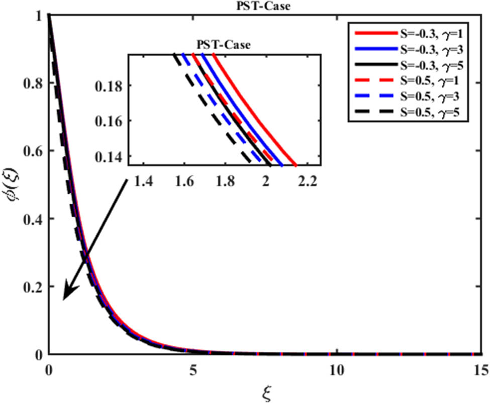
Interaction of suction and injection on Ferro–Jaffery fluid within the

Interaction of suction and injection on Ferro–Jaffery fluid within the
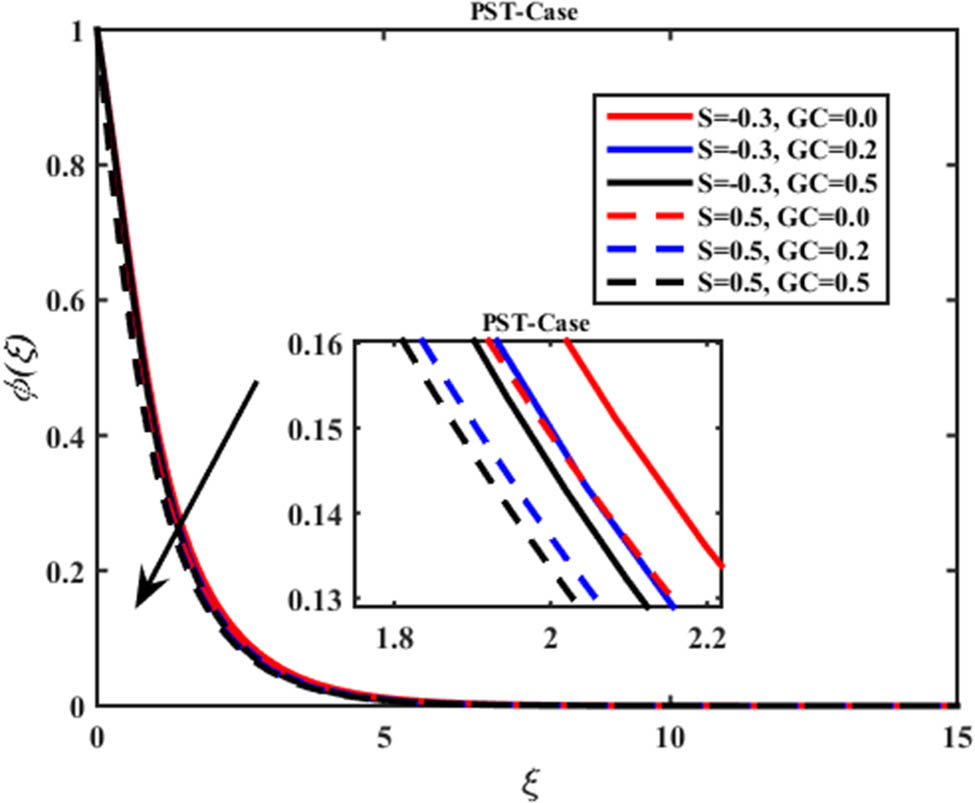
Interaction of suction and injection on Ferro–Jaffery fluid within the GC on concentration profile

Interaction of suction and injection on Ferro–Jaffery fluid within the GT on concentration profile
Interaction of suction and injection on Ferro–Jaffery fluid within the

Interaction of suction and injection on Ferro–Jaffery fluid within the

Interaction of suction and injection on Ferro–Jaffery fluid within the
5 Conclusion
This research signifies into the two-dimensional flow with heat and mass transfers of Jeffrey fluid encountering thermal radiation and heat source–sink effects over a linearly inclined vertical stretched sheet under Stefan blowing conditions. It examines the influence of a magnetic dipole under two distinct thermal processes: PST and PHF. Moreover, these thermal and concentration characteristics are further enhanced by incorporating the Darcy–Forchheimer model, mixed convection, the Buongiorno fluid model, and slip conditions. The comprehension of BL flow and heat transfer with mixed convection holds significant importance across various industries due to the challenges in achieving desired product outcomes from these processes. The study aims to elucidate the impact of viscous dissipation, Soret and Dufour effects, and a magnetic dipole on flow and heat transfer in Jeffrey fluid along an inclined vertical stretching surface. To enhance the rheological model, it incorporates thermophoresis, Brownian motion, and chemical reaction effects for an improved concentration profile. Utilizing similarity transformations, the model equations are converted into coupled nonlinear ODEs. The BVP4C method is then applied to derive solutions for the fluid’s velocity and temperature. The analysis conducted through the similarity transformations sheds light on the influence of various physical parameters on the flow field, as described by the BVP equations. Key findings from the discussion and figures can be summarized as follows:
Fluid velocity rises with increasing
Velocity decreases with higher
Velocity increases with higher Da values during suction and decreases during injection (Figure 5).
Velocity rises with higher Fr values during injection and falls during suction (Figure 7).
Temperature increases slowly with higher
Temperature increases with higher Nt and
Temperature rises with higher Pr values and falls with higher
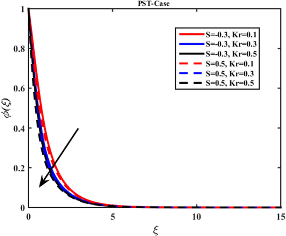
Concentration decreases with higher
Concentration increases with higher
Concentration increases with higher Pr and Nb values (Figures 31 and 32).
6 Applications
The mathematical analysis of Jeffrey FMFs on vertical inclined stretched surfaces with Darcy–Forchheimer and mixed convection effects has several applications, including:
Magnetic drug targeting: FMFs can be used to deliver drugs to specific locations in the body using magnetic fields. The analysis of their flow behavior is crucial for optimizing the drug delivery process.
Heat transfer enhancement: FMFs can be used as coolants in various applications due to their enhanced heat transfer properties. The analysis helps in designing efficient cooling systems.
Lubrication and bearing systems: FMFs can be used as lubricants in bearings and other mechanical systems. The analysis helps in understanding their behavior under different operating conditions.
Microfluidics and lab-on-a-chip devices: FMFs can be used in microfluidic devices for various applications, such as valves and pumps. The analysis helps in designing and optimizing these devices.
The mathematical analysis of Jeffrey FMFs on vertical inclined stretched surfaces with Darcy–Forchheimer and mixed convection effects provides valuable insights into the behavior of these fluids under specific conditions. It helps in understanding the complex interactions between the fluid, magnetic field, and the surrounding environment, which is crucial for developing and optimizing various applications involving FMFs.
7 Future direction
The ongoing research needs to examine Jeffrey’s FMF flow behavior under unsteady three-dimensional conditions with advanced boundary setups. A study of thermal transport mechanisms would benefit from analyzing non-Fourier heat transfer models including the Cattaneo–Christov heat flux. The thermal and concentration characteristics become stronger through research incorporation of adjustable magnetic field strength together with anisotropic porous permeability and hybrid nanofluids solutions. The prediction and optimization of actual-world flow behavior could be achieved through machine learning methods that select appropriate parameters. Laboratory testing of research-based findings will prove beneficial for developing real-world cooling applications that serve biomedical medicine and aerospace and industrial sectors.
Acknowledgment
The authors gratefully acknowledge the support of their respective institutions for providing the necessary resources and research environment that facilitated the completion of this work. The authors also thank the reviewers and editors of Nonlinear Engineering for their valuable feedback and constructive comments, which have significantly improved the quality of this manuscript.
-
Funding information: The authors state no funding involved.
-
Author contributions: All authors have accepted responsibility for the entire content of this manuscript and approved its submission.
-
Conflict of interest: The authors state no conflict of interest.
-
Data availability statement: All data generated or analysed during this study are included in this published article.
References
[1] Guo N, Du H, Li W. Finite element analysis and simulation evaluation of a magnetorheological valve. Int J Adv Manuf Technol. 2003;21:438–45. 10.1007/s001700300051Suche in Google Scholar
[2] Kumar JS, Paul PS, Raghunathan G, Alex DG. A review of challenges and solutions in the preparation and use of magnetorheological fluids. Int J Mech Mater Eng. 2019;14(1):13. 10.1186/s40712-019-0109-2Suche in Google Scholar
[3] Mitamura Y, Sekine K, Okamoto E. Magnetic fluid seals working in liquid environments: factors limiting their life and solution methods. J Magn Magn Mater. 2020;500:166293. 10.1016/j.jmmm.2019.166293Suche in Google Scholar
[4] Nakatsuka K. Trends of magnetic fluid applications in Japan. J Magn Magn Mater. 1993;122(1–3):387–94. 10.1016/0304-8853(93)91116-OSuche in Google Scholar
[5] Arefyev MI, Demidenko VO, Saikin MS. Assessment of magnetic fluid stability in non-homogeneous magnetic field of a single-tooth magnetic fluid sealer. J Magn Magn Mater. 2017;431:20–3. 10.1016/j.jmmm.2016.10.017Suche in Google Scholar
[6] Yamaguchi H, Bessho T. Long distance heat transport device using temperature sensitive magnetic fluid. J Magn Magn Mater. 2020;499:166248. 10.1016/j.jmmm.2019.166248. Suche in Google Scholar
[7] Khan SA, Suresh A, Ramaiah NS. Principles, characteristics and applications of magneto rheological fluid damper in flow and shear mode. Proc Mat Sci. 2014;6:1547–56. 10.1016/j.mspro.2014.07.136Suche in Google Scholar
[8] Lagutkina DY, Saikin MS. The research and development of inclination angle magnetic fluid detector with a movable sensing element based on permanent magnets. J Magn Magn Mater. 2017;431:149–51. 10.1016/j.jmmm.2016.11.040Suche in Google Scholar
[9] Xie J, Li D, Xing YA. The theoretical and experimental investigation on the vertical magnetic fluid pressure sensor. Sensor Actuat A-Phys. 2015;229:42–9. 10.1016/j.sna.2015.03.007Suche in Google Scholar
[10] Kumar CSSR, Mohammad F. Magnetic nanomaterials for hyperthermia-based therapy and controlled drug delivery. Adv Drug Deliver Rev. 2011;63(9):789–808. 10.1016/j.addr.2011.03.008Suche in Google Scholar PubMed PubMed Central
[11] Hedayati N, Ramiar A, Larimi MM. Investigating the effect of external uniform magnetic field and temperature gradient on the uniformity of nanoparticles in drug delivery applications. J Mol Liq. 2018;272:301–12. 10.1016/j.molliq.2018.09.031Suche in Google Scholar
[12] Bernad SI, Craciunescu I, Sandhu GS, Dragomir-Daescu D, Tombacz E, Vekas L, et al. Fluid targeted delivery of functionalized magnetoresponsive nanocomposite particles to a ferromagnetic stent. J Magnet Magnetic Mater. 2021;519:167489. 10.1016/j.jmmm.2020.167489Suche in Google Scholar
[13] Kandasamy G, Khan S, Giri J, Bose S, Veerapu NS, Maity D. One-pot synthesis of hydrophilic flower-shaped iron oxide nanoclusters (IONCs) based ferrofluids for magnetic fluid hyperthermia applications. J Mol Liq. 2019;275:699–712. 10.1016/j.molliq.2018.11.108Suche in Google Scholar
[14] Liu XL, Fan HM, Innovative magnetic nanoparticle platform for magnetic resonance imaging and magnetic fluid hyperthermia applications. Curr Opin Chem Eng. 2014;4:38–46. 10.1016/j.coche.2013.12.010Suche in Google Scholar
[15] Andersson HI, Valnes OA. Flow of a heated ferrofluid over a stretching sheet in the presence of a magnetic dipole. Acta Mech. 1998;128(1):39–47. 10.1007/BF01463158Suche in Google Scholar
[16] Yellen BB, Fridman G, Friedman G. Ferrofluid lithography. Nanotechnology. 2004;15(10):S562–5. 10.1088/0957-4484/15/10/011Suche in Google Scholar
[17] Chang CH, Tan CW, Miao J, Barbastathis G. Self-assembled ferrofluid lithography: patterning micro and nanostructures by controlling magnetic nanoparticles. Nanotechnology. 2009;20(49):495301. 10.1088/0957-4484/20/49/495301Suche in Google Scholar PubMed
[18] Zeeshan A, Majeed A, Ellahi R. Effect of magnetic dipole on viscous ferro-fluid past a stretching surface with thermal radiation. J Mol Liq. 2016;215:549–54. 10.1016/j.molliq.2015.12.110Suche in Google Scholar
[19] Sohail A, Fatima M, Ellahi R, Akram KB. A videographic assessment of ferrofluid during magnetic drug targeting: an application of artificial intelligence in nanomedicine. J Mol Liq. 2019;285:47–57. 10.1016/j.molliq.2019.04.022Suche in Google Scholar
[20] Kumar RN, Gowda RJP, Abusorrah AM, Mahrous MY, Abu-Hamdeh NH, Issakhov A, et al. Impact of magnetic dipole on ferromagnetic hybrid nanofluid flow over a stretching cylinder. Phys Scr. 2021;96(4):045215. 10.1088/1402-4896/abe324Suche in Google Scholar
[21] Almaneea A. Thermal analysis for ferromagnetic fluid with hybrid nano-metallic structures in the presence of Forchheirmer porous medium subjected to a magnetic dipole. Case Stud Thermal Eng. 2021;26:100961. 10.1016/j.csite.2021.100961Suche in Google Scholar
[22] Gowda RJP, Kumar RN, Prasannakumara BC, Nagaraja B, Gireesha BJ. Exploring magnetic dipole contribution on ferromagnetic nanofluid flow over a stretching sheet: An application of Stefan blowing. J Molecular Liquids. 2021;335:116215. 10.1016/j.molliq.2021.116215Suche in Google Scholar
[23] Hussain I, Hobiny A, Irfan M, Tabrez M, Khan WA. Impact of magnetic dipole contribution on radiative ferromagnetic Cross nanofluid flow with viscous dissipation aspects. J Magnetism Magnetic Materials. 2023;579:170706. 10.1016/j.jmmm.2023.170706Suche in Google Scholar
[24] Zeeshan A, Majeed A. Heat transfer analysis of Jeffery fluid flow over a stretching sheet with suction/injection and magnetic dipole effect. Alexandr Eng J. 2016;55:2171–81. 10.1016/j.aej.2016.06.014Suche in Google Scholar
[25] Yasmeen S, Asghar S, Anjum HJ, Ehsan T. Analysis of Hartmann boundary layer peristaltic flow of Jeffrey fluid: Quantitative and qualitative approaches. Commun Nonlinear Sci Numer Simulat. 2019;76:51–65. 10.1016/j.cnsns.2019.01.007Suche in Google Scholar
[26] Abbas N, Ali M, Abodayeh K, Mustafa Z, Shatanawi W. Thermal investigation of Jeffrey fluid flow past a stretching Riga curved surface under Soret and Dufour impacts. Case Stud Thermal Eng. 2023;52:103553. 10.1016/j.csite.2023.103553Suche in Google Scholar
[27] Ashraf H, Shah NA, Siddiqui AM, Rehman H, Turki NB. Analysis of heat transfer in n-immiscible layers of a horizontal Jeffrey fluid film flow. Case Stud Thermal Eng. 2023;51:103662. 10.1016/j.csite.2023.103662Suche in Google Scholar
[28] Ullah H, Alqahtani AM, Raja MAZ, Fiza M, Ullah M, Abdoalrahman, et al. Numerical treatment based on artificial neural network to Soret and Dufour effects on MHD squeezing flow of Jeffrey fluid in horizontal channel with thermal radiation. Int J Thermofluids. 2024;23:100725. 10.1016/j.ijft.2024.100725Suche in Google Scholar
[29] Muzammal M, Farooq M, Hashim, Alotaibi H. Transportation of melting heat in stratified Jeffrey fluid flow with heat generation and magnetic field. Case Stud Thermal Eng. 2024;58:104465. 10.1016/j.csite.2024.104465Suche in Google Scholar
[30] Li D, Li H, Ma L, Lan S. Oscillating flow of Jeffrey fluid in a rough circular microchannel with slip boundary condition. Chin J Phys. 2024;91:107–29. 10.1016/j.cjph.2024.07.015Suche in Google Scholar
[31] Darcy H. Les Fontaines Publiques De La Ville De Dijon. Paris: VictorDalmont; 1856. Suche in Google Scholar
[32] Forchheimer P. Wasserbewegung durch Boden. Spielhagen Schurich. 1901;45:1782–8. https://ci.nii.ac.jp/naid/10010395788. Suche in Google Scholar
[33] Al-arabi TH, Eid MR, Alsemiry RD, Alharbi SA, Allogmany R, Elsaid EM. Electromagnetic and Darcy–Forchheimer porous model effects on hybrid nanofluid flow in conical zone of rotatable cone and expandable disc. Alex Eng J. 2004;96:206–17. 10.1016/j.aej.2024.04.007Suche in Google Scholar
[34] Prakash J, Tripathi D, Tiwari AK, Pandey AK. Melting heat transfer and irreversibility analysis in Darcy–Forchheimer flow of Casson fluid modulated by EMHD over cone and wedge surfaces. Therm Sci Eng Progress. 2024;52:102680. 10.1016/j.tsep.2024.102680Suche in Google Scholar
[35] Ramana RM, Dharmaiah G, Kumar MS, Fernandez-Gamiz U, Noeiaghdam S. Numerical performance of Hall current and Darcy–Forchheimer influences on dissipative Newtonian fluid flow over a thinner surface. Case Stud Thermal Eng. 2024;60:104687. 10.1016/j.csite.2024.104687Suche in Google Scholar
[36] Salahuddin T, Kalsoom SM, Awais M, Khan M, Altanji M. Impact of Darcy–Forchheimer for the flow analysis of radiated tangent hyperbolic fluid with viscous dissipation and activation energy. Int J Hydrogen Energy. 2024;72:949–57. 10.1016/j.ijhydene.2024.05.425Suche in Google Scholar
[37] Yang L, Du K. A comprehensive review on the natural, forced, and mixed convection of non-Newtonian fluids (nanofluids) inside different cavities. J Thermal Anal Calorim 2020;140:2033–54. 10.1007/s10973-019-08987-ySuche in Google Scholar
[38] Naveed M, Abbas Z, Sajid M. Mixed convection flow of a Casson fluid over a curved stretching surface with nonlinear Rosseland thermal radiation. J Eng Thermophys. 2023;32(4):824–34. 10.1134/S1810232823040148Suche in Google Scholar
[39] Algehyne EA, Alamrani FM, Alrabaiah H, Lone SA, Yasmin H, Saeed A. Comparative analysis on the forced and mixed convection in a hybrid nanofuid fow over a stretching surface: a numerical analysis. J Thermal Anal Calorimetry. 2024. https://doi.org/10.1007/s10973-024-13178-5. Suche in Google Scholar
[40] Mandal IC, Mukhopadhyay S, Mandal MS. MHD mixed convective Maxwell liquid flow passing an unsteady stretched sheet. Partial Differ Equ Appl Math. 2024;9:100644. 10.1016/j.padiff.2024.100644Suche in Google Scholar
[41] Deb N, Saha S. Role of internal heat generation, magnetism and Joule heating on entropy generation and mixed convective flow in a square domain. Annals of Nuclear Energy. 2024;198:110324. 10.1016/j.anucene.2023.110324Suche in Google Scholar
[42] Alali Z, Eckels SJ. 3D numerical simulations of mixed convective heat transfer and correlation development for a thermal manikin head. Heliyon. 2024;10:e30161. 10.1016/j.heliyon.2024.e30161Suche in Google Scholar PubMed PubMed Central
[43] Devi MM, Sivakumar N, Noeiaghdam S, Fernandez-Gamiz U. Multiple shape factor effects of nanofluids on Marangoni mixed convection flow through porous medium. Results Eng. 2024;23:102512. 10.1016/j.rineng.2024.102512Suche in Google Scholar
[44] Ibrahim IU, Sharifpur M, Meye JP. Mixed convection heat transfer characteristics of Al2O3 - MWCNT hybrid nanofluid under thermally developing flow; Effects of particles percentage weight composition. Appl Thermal Eng. 2024;249:123372. 10.1016/j.applthermaleng.2024.123372Suche in Google Scholar
[45] Revathi R, Poornima T. Dynamics of stagnant Sutterby fluid due to mixed convection with an emphasis on thermal analysis. J Thermal Anal Calorimetry. 2024;149:7059–69. 10.1007/s10973-024-12943-wSuche in Google Scholar
[46] A. Hassan. Nanoparticle’s shape effect on mixed convection heat transfer and flow of Carbon nanotubes: Numerical approach. Bio Nano Sci. 2024;14:1627–43. 10.1007/s12668-024-01378-0Suche in Google Scholar
[47] Sarana HL, Reddy CR. Effect of thermal radiation on aqueous hybrid nanofluid: the stability analysis. Eur Phys J. Plus. 2024;139:209. 10.1140/epjp/s13360-024-05027-zSuche in Google Scholar
[48] Alrihielia H. Thermal and concentration slip impact on the dissipative Casson-Maxwell nanofluid flow due to a stretching sheet with heat generation and thermal radiation. Eur Phys J Plus 2023;138:916. 10.1140/epjp/s13360-023-04525-wSuche in Google Scholar
[49] Yedhiri SR, Palaparthi KK, Kodi R, Asmat F. Unsteady MHD rotating mixed convective flow through an infinite vertical plate subject to Joule heating, thermal radiation, Hall current, radiation absorption. J Thermal Anal Calorimetry. 2024;149:8813–26. 10.1007/s10973-024-12954-7Suche in Google Scholar
[50] Rao S, Deka PN. Numerical analysis of MHD Hybrid nanofluid flow a porous stretching sheet with thermal radiation. Int J Appl Comput Math. 2024;10:95. 10.1007/s40819-024-01734-4Suche in Google Scholar
[51] Madhu J, Madhukesh JK, Sarris I, Prasannakumara BC, Ramesh GK, Shah NA, et al. Influence of quadratic thermal radiation and activation energy impacts over oblique stagnation point hybrid nanofluid flow across a cylinder. Case Stud Thermal Eng. 2024;60:104624. 10.1016/j.csite.2024.104624Suche in Google Scholar
[52] Alamirew WD, Awgichew G, Haile E. Mixed convection flow of MHD Casson nanofluid over a vertically extending sheet with effects of Hall, Ion Slip and nonlinear thermal radiation. Int J Thermofluids. 2024;23:100762. 10.1016/j.ijft.2024.100762Suche in Google Scholar
[53] Jiann LY, Mohamad AQ, Rawi NA, Ching DLC, Zin NAM, Shafie S. Thermal analysis of melting effect on Carreau fluid flow around a stretchable cylinder with quadratic radiation. Propulsion Power Res. 2024;13(1):132–43. 10.1016/j.jppr.2024.02.006Suche in Google Scholar
[54] Hussain F, Hussain A, Nadeem S. Thermophoresis and Brownian model of pseudo-plastic nanofuid fow over a vertical slender cylinder. Math Problems Eng. 2020;2020:1–10. 10.1155/2020/8428762Suche in Google Scholar
[55] Shafey AEM, Alharbi FM, Javed A, Abbas N, ALrafai HA, Nadeem, S, et al. Theoretical analysis of Brownian and thermophoresis motion effects for Newtonian fluid flow over nonlinear stretching cylinder. Case Stud Thermal Eng. 2021;28:101369. 10.1016/j.csite.2021.101369Suche in Google Scholar
[56] Tawade JV, Guled CN, Noeiaghdam S, Fernandez-Gamiz U., Govindan V, Balamuralitharan S. Effects of thermophoresis and Brownian motion for thermal and chemically reacting Casson nanofluid flow over a linearly stretching sheet. Results Eng. 2022;15:100448. 10.1016/j.rineng.2022.100448Suche in Google Scholar
[57] Sarfraz M, Khan M, Ahmed A. Study of thermophoresis and Brownian motion phenomena in radial stagnation flow over a twisting cylinder. Ain Shams Eng J. 2023;14(2):101869. 10.1016/j.asej.2022.101869Suche in Google Scholar
[58] Jawad M, Ghazwani HA. Inspiration of Thermophoresis and Brownian motion on magneto hydrodynamic flow over a cylinder fixed with porous medium. Bio Nano Sci. 2023;13:2122–33. 10.1007/s12668-023-01229-4Suche in Google Scholar
[59] Sharma K, Vijay N, D. Bhardwaj D, Jindal R. Flow of water conveying Fe3O4 and Mn-ZnFe2O4 nanoparticles over a rotating disk: Significance of thermophoresis and Brownian motion. J Magnetism Magnetic Materials. 2023;574:170710. 10.1016/j.jmmm.2023.170710Suche in Google Scholar
[60] Khan D, Ali G, Kumam P, Sitthithakerngkiet K, Jarad F. Heat transfer analysis of unsteady MHD slip flow of ternary hybrid Casson fluid through nonlinear stretching disk embedded in a porous medium. Ain Shams Eng J. 2023;15(2):102419. 10.1016/j.asej.2023.102419Suche in Google Scholar
[61] Khan D, Ali G, Kumam P, Jarad F. An exploration of heat and mass transfer for MHD flow of Brinkman type dusty fluid between fluctuating parallel vertical plates with arbitrary wall shear stress. Int J Thermofluids. 2024;21:100529. 10.1016/j.ijft.2023.100529Suche in Google Scholar
[62] Khan D, Kumam P, Khan I, Sitthithakerngkiet K, Khan A, Ali, G. Unsteady rotating MHD flow of a second-grade hybrid nanofluid in a porous medium: Laplace and Sumudu transforms. Heat Transfer. 2022;51:8065–83. 10.1002/htj.22681Suche in Google Scholar
[63] Khan I, Khan D, Ali G, Khan, A. Effect of Newtonian heating on two-phase fluctuating flow of dusty fluid: Poincaré-Lighthill perturbation technique. European Phys J Plus. 2021;136:1142. 10.1140/epjp/s13360-021-02101-8Suche in Google Scholar
[64] Khan D, Ali G, Kumam P, Suttiarporn P. A generalized electro-osmotic MHD flow of hybrid ferrofluid through Fourier and Fickas law in inclined microchannel. Numer Heat Transfer Part A Appl. 2024;85:3091–109. 10.1080/10407782.2023.2232535Suche in Google Scholar
[65] Khan D, Ali G, Kumam P, Almusawa M. Y, Galal A. M. Time fractional model of free convection flow and dusty two-phase couple stress fluid along vertical plates. ZAMM - J Appl Math Mechanics/Zeitschrift für Angewandte Mathematik und Mechanik. 2022;103:e202200369. 10.1002/zamm.202200369Suche in Google Scholar
[66] Khan D, Ali G, Ghazwani HA. Enhancing heat transfer in MHD Falkneras-Skan flow with thermal radiation, free convection and dusty fluid between parallel plates. Heat Transfer. 2024;53:1408–24. 10.1002/htj.23002Suche in Google Scholar
[67] Chen C. Laminar mixed convection adjacent to vertical, continuously stretching sheets. Heat Mass Transfer. 1998;33:471–76. 10.1007/s002310050217Suche in Google Scholar
[68] Abel MS, Sanjayanand E, Nandeppanavar MM. Viscoelastic MHD flow and heat transfer over a stretching sheet with viscous and ohmic dissipations. Commun Nonl Sci Numer Simulat. 2008;13:1808–21. 10.1016/j.cnsns.2007.04.007Suche in Google Scholar
[69] Agarwal K, Baghel RS, Parmar A, Dadheech A. Jeffery Slip Fluid Flow with the Magnetic Dipole Effect Over a Melting or Permeable Linearly Stretching Sheet. Int J Appl Comput Math. 2024;10:5. 10.1007/s40819-023-01629-wSuche in Google Scholar
© 2025 the author(s), published by De Gruyter
This work is licensed under the Creative Commons Attribution 4.0 International License.
Artikel in diesem Heft
- Research Articles
- Generalized (ψ,φ)-contraction to investigate Volterra integral inclusions and fractal fractional PDEs in super-metric space with numerical experiments
- Solitons in ultrasound imaging: Exploring applications and enhancements via the Westervelt equation
- Stochastic improved Simpson for solving nonlinear fractional-order systems using product integration rules
- Exploring dynamical features like bifurcation assessment, sensitivity visualization, and solitary wave solutions of the integrable Akbota equation
- Research on surface defect detection method and optimization of paper-plastic composite bag based on improved combined segmentation algorithm
- Impact the sulphur content in Iraqi crude oil on the mechanical properties and corrosion behaviour of carbon steel in various types of API 5L pipelines and ASTM 106 grade B
- Unravelling quiescent optical solitons: An exploration of the complex Ginzburg–Landau equation with nonlinear chromatic dispersion and self-phase modulation
- Perturbation-iteration approach for fractional-order logistic differential equations
- Variational formulations for the Euler and Navier–Stokes systems in fluid mechanics and related models
- Rotor response to unbalanced load and system performance considering variable bearing profile
- DeepFowl: Disease prediction from chicken excreta images using deep learning
- Channel flow of Ellis fluid due to cilia motion
- A case study of fractional-order varicella virus model to nonlinear dynamics strategy for control and prevalence
- Multi-point estimation weldment recognition and estimation of pose with data-driven robotics design
- Analysis of Hall current and nonuniform heating effects on magneto-convection between vertically aligned plates under the influence of electric and magnetic fields
- A comparative study on residual power series method and differential transform method through the time-fractional telegraph equation
- Insights from the nonlinear Schrödinger–Hirota equation with chromatic dispersion: Dynamics in fiber–optic communication
- Mathematical analysis of Jeffrey ferrofluid on stretching surface with the Darcy–Forchheimer model
- Exploring the interaction between lump, stripe and double-stripe, and periodic wave solutions of the Konopelchenko–Dubrovsky–Kaup–Kupershmidt system
- Computational investigation of tuberculosis and HIV/AIDS co-infection in fuzzy environment
- Signature verification by geometry and image processing
- Theoretical and numerical approach for quantifying sensitivity to system parameters of nonlinear systems
- Chaotic behaviors, stability, and solitary wave propagations of M-fractional LWE equation in magneto-electro-elastic circular rod
- Dynamic analysis and optimization of syphilis spread: Simulations, integrating treatment and public health interventions
- Visco-thermoelastic rectangular plate under uniform loading: A study of deflection
- Threshold dynamics and optimal control of an epidemiological smoking model
- Numerical computational model for an unsteady hybrid nanofluid flow in a porous medium past an MHD rotating sheet
- Regression prediction model of fabric brightness based on light and shadow reconstruction of layered images
- Dynamics and prevention of gemini virus infection in red chili crops studied with generalized fractional operator: Analysis and modeling
- Qualitative analysis on existence and stability of nonlinear fractional dynamic equations on time scales
- Fractional-order super-twisting sliding mode active disturbance rejection control for electro-hydraulic position servo systems
- Analytical exploration and parametric insights into optical solitons in magneto-optic waveguides: Advances in nonlinear dynamics for applied sciences
- Bifurcation dynamics and optical soliton structures in the nonlinear Schrödinger–Bopp–Podolsky system
- User profiling in university libraries by combining multi-perspective clustering algorithm and reader behavior analysis
- Exploring bifurcation and chaos control in a discrete-time Lotka–Volterra model framework for COVID-19 modeling
- Review Article
- Haar wavelet collocation method for existence and numerical solutions of fourth-order integro-differential equations with bounded coefficients
- Special Issue: Nonlinear Analysis and Design of Communication Networks for IoT Applications - Part II
- Silicon-based all-optical wavelength converter for on-chip optical interconnection
- Research on a path-tracking control system of unmanned rollers based on an optimization algorithm and real-time feedback
- Analysis of the sports action recognition model based on the LSTM recurrent neural network
- Industrial robot trajectory error compensation based on enhanced transfer convolutional neural networks
- Research on IoT network performance prediction model of power grid warehouse based on nonlinear GA-BP neural network
- Interactive recommendation of social network communication between cities based on GNN and user preferences
- Application of improved P-BEM in time varying channel prediction in 5G high-speed mobile communication system
- Construction of a BIM smart building collaborative design model combining the Internet of Things
- Optimizing malicious website prediction: An advanced XGBoost-based machine learning model
- Economic operation analysis of the power grid combining communication network and distributed optimization algorithm
- Sports video temporal action detection technology based on an improved MSST algorithm
- Internet of things data security and privacy protection based on improved federated learning
- Enterprise power emission reduction technology based on the LSTM–SVM model
- Construction of multi-style face models based on artistic image generation algorithms
- Research and application of interactive digital twin monitoring system for photovoltaic power station based on global perception
- Special Issue: Decision and Control in Nonlinear Systems - Part II
- Animation video frame prediction based on ConvGRU fine-grained synthesis flow
- Application of GGNN inference propagation model for martial art intensity evaluation
- Benefit evaluation of building energy-saving renovation projects based on BWM weighting method
- Deep neural network application in real-time economic dispatch and frequency control of microgrids
- Real-time force/position control of soft growing robots: A data-driven model predictive approach
- Mechanical product design and manufacturing system based on CNN and server optimization algorithm
- Application of finite element analysis in the formal analysis of ancient architectural plaque section
- Research on territorial spatial planning based on data mining and geographic information visualization
- Fault diagnosis of agricultural sprinkler irrigation machinery equipment based on machine vision
- Closure technology of large span steel truss arch bridge with temporarily fixed edge supports
- Intelligent accounting question-answering robot based on a large language model and knowledge graph
- Analysis of manufacturing and retailer blockchain decision based on resource recyclability
- Flexible manufacturing workshop mechanical processing and product scheduling algorithm based on MES
- Exploration of indoor environment perception and design model based on virtual reality technology
- Tennis automatic ball-picking robot based on image object detection and positioning technology
- A new CNN deep learning model for computer-intelligent color matching
- Design of AR-based general computer technology experiment demonstration platform
- Indoor environment monitoring method based on the fusion of audio recognition and video patrol features
- Health condition prediction method of the computer numerical control machine tool parts by ensembling digital twins and improved LSTM networks
- Establishment of a green degree evaluation model for wall materials based on lifecycle
- Quantitative evaluation of college music teaching pronunciation based on nonlinear feature extraction
- Multi-index nonlinear robust virtual synchronous generator control method for microgrid inverters
- Manufacturing engineering production line scheduling management technology integrating availability constraints and heuristic rules
- Analysis of digital intelligent financial audit system based on improved BiLSTM neural network
- Attention community discovery model applied to complex network information analysis
- A neural collaborative filtering recommendation algorithm based on attention mechanism and contrastive learning
- Rehabilitation training method for motor dysfunction based on video stream matching
- Research on façade design for cold-region buildings based on artificial neural networks and parametric modeling techniques
- Intelligent implementation of muscle strain identification algorithm in Mi health exercise induced waist muscle strain
- Optimization design of urban rainwater and flood drainage system based on SWMM
- Improved GA for construction progress and cost management in construction projects
- Evaluation and prediction of SVM parameters in engineering cost based on random forest hybrid optimization
- Museum intelligent warning system based on wireless data module
- Optimization design and research of mechatronics based on torque motor control algorithm
- Special Issue: Nonlinear Engineering’s significance in Materials Science
- Experimental research on the degradation of chemical industrial wastewater by combined hydrodynamic cavitation based on nonlinear dynamic model
- Study on low-cycle fatigue life of nickel-based superalloy GH4586 at various temperatures
- Some results of solutions to neutral stochastic functional operator-differential equations
- Ultrasonic cavitation did not occur in high-pressure CO2 liquid
- Research on the performance of a novel type of cemented filler material for coal mine opening and filling
- Testing of recycled fine aggregate concrete’s mechanical properties using recycled fine aggregate concrete and research on technology for highway construction
- A modified fuzzy TOPSIS approach for the condition assessment of existing bridges
- Nonlinear structural and vibration analysis of straddle monorail pantograph under random excitations
- Achieving high efficiency and stability in blue OLEDs: Role of wide-gap hosts and emitter interactions
- Construction of teaching quality evaluation model of online dance teaching course based on improved PSO-BPNN
- Enhanced electrical conductivity and electromagnetic shielding properties of multi-component polymer/graphite nanocomposites prepared by solid-state shear milling
- Optimization of thermal characteristics of buried composite phase-change energy storage walls based on nonlinear engineering methods
- A higher-performance big data-based movie recommendation system
- Nonlinear impact of minimum wage on labor employment in China
- Nonlinear comprehensive evaluation method based on information entropy and discrimination optimization
- Application of numerical calculation methods in stability analysis of pile foundation under complex foundation conditions
- Research on the contribution of shale gas development and utilization in Sichuan Province to carbon peak based on the PSA process
- Characteristics of tight oil reservoirs and their impact on seepage flow from a nonlinear engineering perspective
- Nonlinear deformation decomposition and mode identification of plane structures via orthogonal theory
- Numerical simulation of damage mechanism in rock with cracks impacted by self-excited pulsed jet based on SPH-FEM coupling method: The perspective of nonlinear engineering and materials science
- Cross-scale modeling and collaborative optimization of ethanol-catalyzed coupling to produce C4 olefins: Nonlinear modeling and collaborative optimization strategies
- Unequal width T-node stress concentration factor analysis of stiffened rectangular steel pipe concrete
- Special Issue: Advances in Nonlinear Dynamics and Control
- Development of a cognitive blood glucose–insulin control strategy design for a nonlinear diabetic patient model
- Big data-based optimized model of building design in the context of rural revitalization
- Multi-UAV assisted air-to-ground data collection for ground sensors with unknown positions
- Design of urban and rural elderly care public areas integrating person-environment fit theory
- Application of lossless signal transmission technology in piano timbre recognition
- Application of improved GA in optimizing rural tourism routes
- Architectural animation generation system based on AL-GAN algorithm
- Advanced sentiment analysis in online shopping: Implementing LSTM models analyzing E-commerce user sentiments
- Intelligent recommendation algorithm for piano tracks based on the CNN model
- Visualization of large-scale user association feature data based on a nonlinear dimensionality reduction method
- Low-carbon economic optimization of microgrid clusters based on an energy interaction operation strategy
- Optimization effect of video data extraction and search based on Faster-RCNN hybrid model on intelligent information systems
- Construction of image segmentation system combining TC and swarm intelligence algorithm
- Particle swarm optimization and fuzzy C-means clustering algorithm for the adhesive layer defect detection
- Optimization of student learning status by instructional intervention decision-making techniques incorporating reinforcement learning
- Fuzzy model-based stabilization control and state estimation of nonlinear systems
- Optimization of distribution network scheduling based on BA and photovoltaic uncertainty
- Tai Chi movement segmentation and recognition on the grounds of multi-sensor data fusion and the DBSCAN algorithm
- Special Issue: Dynamic Engineering and Control Methods for the Nonlinear Systems - Part III
- Generalized numerical RKM method for solving sixth-order fractional partial differential equations