Bifurcation dynamics and optical soliton structures in the nonlinear Schrödinger–Bopp–Podolsky system
-
Shabbir Hussain


Abstract
In this article, the complex structure of optical soliton solutions of the nonlinear Schrödinger–Bopp–Podolsky system is investigated using the enhanced modified extended tanh-expansion approach. It also analyzes the system’s stability and how it changes by performing a bifurcation analysis. This system holds special importance in nonlinear optics because it describes light-wave behavior when they interact with nonlinear materials. The enhanced modified extended tanh-expansion method serves as a strong analytical method to construct numerous innovative and diverse optical solitons including dark and bright and singular types. The obtained solutions help researchers understand all aspects that influence the nonlinear Schrödinger–Bopp–Podolsky system behavior while providing tools for simulating nonlinear optical processes. The potential for discovering new types of optical soliton solutions specific to the Schrödinger–Bopp–Podolsky system, which may differ from those found in other systems, remains untapped. While the current literature demonstrates the effectiveness of the enhanced modified extended tanh-method in various contexts, its application to the nonlinear Schrödinger–Bopp–Podolsky system could provide new insights and expand the understanding of soliton dynamics in modified nonlinear systems.This study is innovative because it is the first to apply the enhanced modified extended tanh-method to the nonlinear Schrödinger–Bopp–Podolsky system. This approach enables the construction of new soliton solutions and provides a deeper understanding of the nonlinear dynamics of the system. We employed Mathematica and MATLAB together to provide comprehensive, illustrative, and high-quality visualizations of the findings for graphical representation.
1 Introduction
The intricate soliton dynamics of the nonlinear Schrödinger–Bopp–Podolsky system are essential for simulating stable, localized wave structures in nonlinear optics and Bose–Einstein condensates. These dynamics reveal how wave-potential interactions lead to phenomena like self-focusing, pattern formation, and energy transfer, impacting applications in quantum technologies and photonics. The nonlinear Schrödinger–Bopp–Podolsky system, coupling the Schrödinger equation with Bopp–Podolsky electrodynamics, has been extensively studied since d’Avenia and Siciliano’s 2019 foundational work, which established a functional framework for electrostatic solutions in
The objective of this study is to construct exact soliton solutions of the Schrödinger–Bopp–Podolsky system using the enhanced modified mxtended tanh-method and to analyze their stability through bifurcation analysis of key parameters. This study fills the gap in understanding the nonlinear Schrödinger–Bopp–Podolsky system’s complex soliton dynamics by constructing new solutions via the enhanced modified extended tanh-method and mapping their stability through bifurcation analysis of key parameters
The methods for obtaining exact explicit soliton solutions of nonlinear partial differential equations are the tanh-function method [22], the exp-function method [23], the extended modified rational expansion method [24], extension of modified rational [25,26], expansion approach improved F-expansion method [27], extended simple equation technique [28], extension of simple equation technique [29], auxiliary equation approach [30,31], extended generalized Riccati equation mapping method [32], unified solver method [33,34], Sardar sub-equation method [35], Jacobi elliptic function method [36], and new mapping method [37].
In this article, we are interested in applying the enhanced modified extended tanh-method for solving the presented model trying to reveal their complex dynamics. The enhanced modified extended tanh-method [38–42] is chosen because it provides a unified framework for construction a broad range of exact soliton solutions, including bright, dark, and singular solitons, for nonlinear partial differential equations like the nonlinear Schrödinger–Bopp–Podolsky system. Compared to standard tanh or sine-cosine methods, it handles more general nonlinearities and yields closed-form results with high efficiency. This flexibility makes it well suited for capturing the rich variety of soliton structures present in the model. Additionally, the method might present novel types of solutions, advancing the discipline. The enhanced modified extended tanh-method is a potent tool for studying nonlinear partial differential equations as a result, and it can significantly enhance research in this area. The enhanced modified extended tanh-method has been successfully applied to the (3+1)-dimensional generalized KdV-ZK equation yielding a variety of soliton solutions, including bright, singular, and periodic solitons [42]. It has also been used to extract exact travelling wave solutions for perturbed nonlinear Schrödinger equations with Kudryashov’s law of refractive index, producing solutions such as bright, dark, and singular solitons [43]. The method has been employed to derive soliton solutions for higher-order (2+1)-dimensional Schrödinger equations with fractional derivatives, demonstrating its versatility in handling complex physical phenomena. Despite its success in other contexts, the application of the enhanced modified extended tanh-expansion method to the nonlinear Schrödinger–Bopp–Podolsky system remains unexplored.
The bifurcation analysis [44–46] performed on this system contributes information about solution alterations during variations in system parameters. Solution structural changes become visible to bifurcation theory when researchers study conditions that construct new solution branches and generate existing solution instability. An essential analysis of solutions is vital because it shows how optical soliton dynamics perform within the nonlinear Schrödinger–Bopp–Podolsky system.
2 Algorithm for enhanced modified extended tanh-expansion method
The enhanced modified extended tanh-method [38–42] algorithm is presented in this section. Below is a summary of our method’s primary steps.
Suppose we have the following nonlinear partial differential equation:
where
Step 1. For traveling wave solutions, apply the following wave transformation:
where
Step 2. Substituting Eq. (2.2) into Eq. (2.1) yields a nonlinear ordinary differential equation:
Step 3. Now let
where
where
Step 4. The homogeneous balance between the highest order derivatives and the nonlinear variables in Eq. (2.3) is utilized to determine the value of the positive integers
Step 5. A system of algebraic equations with regard to
Step 6. The generic form of the optical solitons of Eq. (2.6), which accepts the following solutions, is obtained by solving the algebraic system of equations and then inserting the solutions into Eqs. (2.4) and (2.5)
Type-I. When
Type-II. When
where
Type-III. When
3 Application of enhanced modified extended tanh-expansion method
Consider the nonlinear Schrödinger–Bopp–Podolsky system [2,17–21]:
where
To find the optical soliton solutions of the nonlinear Schrödinger–Bopp–Podolsky system, suppose the following wave transformation,
where
Applying homogeneous balance between the highest order derivatives and the nonlinear terms found in Eq. (3.4), i.e.,
We obtained the following system of algebraic equations by plugging Eq. (3.6) into Eq. (3.4) and then gathering all coefficients of
Solving system of algebraic Eq. (3.8) with help of computational software Maple, we obtained the following results:
Similarly, we obtained the following system of algebraic equations by plugging Eq. (3.7) into Eq. (3.5) and then gathering all coefficients of
Similarly solving the system of algebraic equation 3.10 with help of computational software Maple, we obtained the following results:
Now we obtained the following optical soliton solutions of Eq. (3.1) by substituting Eqs. (3.9) and (3.11) into Eqs. (3.6), and (3.7), respectively, and then substituting the resulting equations into (3.2), and (3.3). Additionally, we employ the Eqs. (2.7)–(2.9) for this purpose.
Type-I. When
Type-II. When
Type-III. When
3.1 The graphical representation of optical soliton solutions
In this section, we employ MATLAB and Mathematica for simulation; we plotted three dimensional surface plots, two-dimensional contour plots, and line plots, which illustrate the effects optical soliton solutions of the NLS-BP system, for bright optical soliton, dark optical soliton, kink optical soliton and anti-kink optical soliton. In these visualizations, one can observe how different types of optical solitons behave in spatial and temporal variables and how stable they are with their unique features.
4 Bifurcation analysis
This section provides a bifurcation analysis of the coupled nonlinear ordinary differential equations:
where
A fixed point (or equilibrium point) is a state where the system does not change over time. In our first-order system, this means all derivatives are zero. We need to solve the following system of algebraic equations:
Clearly,
Case 1:
Case 2:
To determine the stability of these fixed points, we linearize the system by computing the Jacobian matrix
We then evaluate the Jacobian at each fixed point and find its eigenvalues. The stability of the fixed point is determined by the real part of these eigenvalues.
If all eigenvalues have negative real parts, the fixed point is asymptotically stable (a sink).
If at least one eigenvalue has a positive real part, the fixed point is unstable (a source or saddle).
If one or more eigenvalues have a zero real part, the linear approximation fails, and this is where a bifurcation might occur.
The eigenvalues are given by the roots of the characteristic equation
A bifurcation will occur at any point where one of these eigenvalues changes sign, such as when
4.1 Graphical representation of bifurcation analysis
A graphical representation of the bifurcation analysis is a great way to visualize how the system’s behavior changes with its parameters. Since our system is four-dimensional, plotting a full phase portrait is not feasible. The most common and effective way to show this is with a bifurcation diagram and simplified 2D-phase portraits (Table 1).
Summary of bifurcation analysis for the coupled
| Parameter | Role in dynamics | Bifurcation indicator | Observed effect (from plots) | Physical meaning |
|---|---|---|---|---|
|
|
Linear stiffness term in
|
Changes sign in
|
Alters phase portrait topology: from single-well to double-well effective potential; critical value where equilibria split | Controls oscillation frequency and onset of symmetry-breaking |
|
|
Nonlinear self-interaction | Appears in cubic term
|
Larger
|
Sets strength of self-focusing/defocusing |
|
|
Linear coupling between
|
Off-diagonal term in Jacobian (
|
Couples
|
Energy exchange between modes |
|
|
Damping (or advection-like) term | Linear in
|
Higher
|
Dissipation or background drift |
5 Physical interpretation of the obtained geometries
5.1 Physical interpretation of the optical soliton solutions
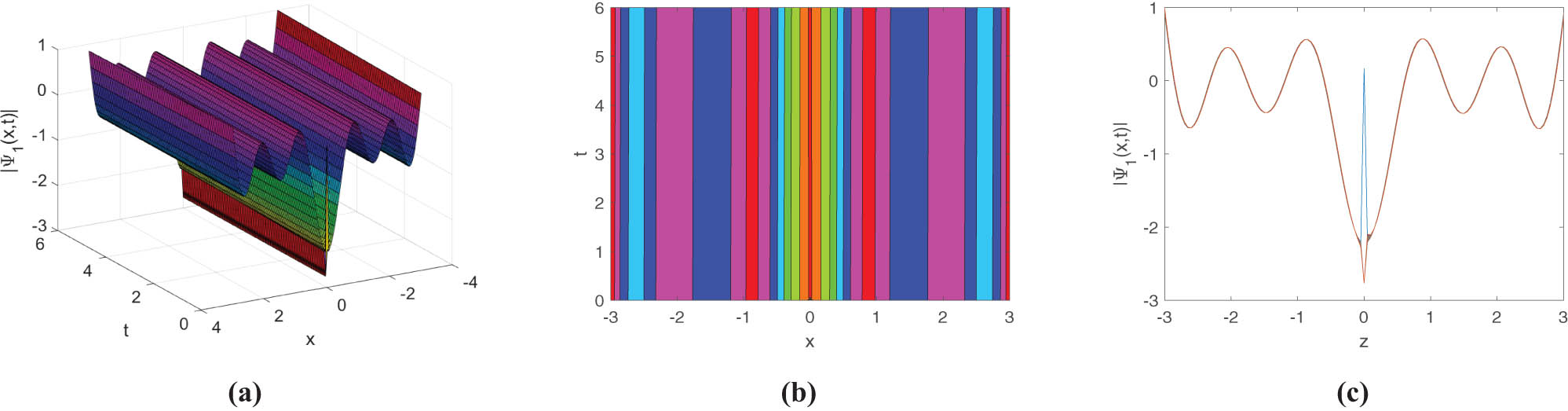
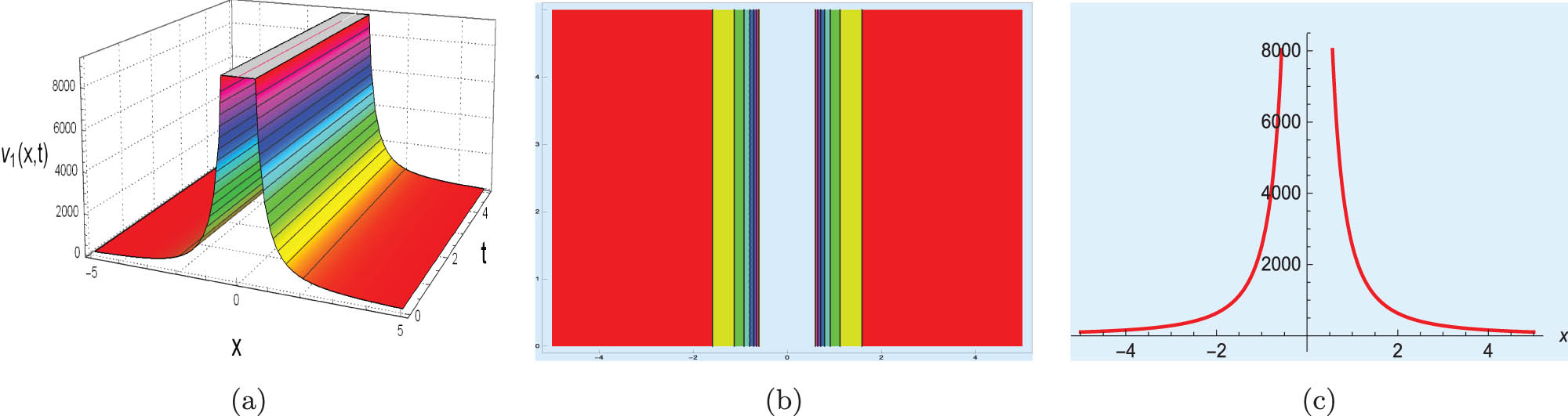
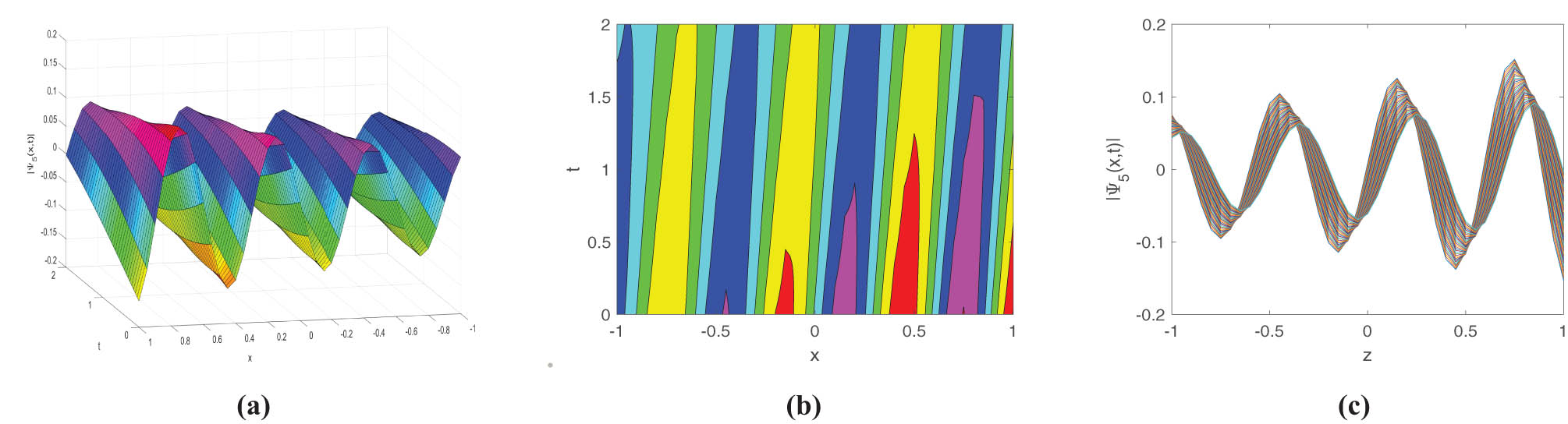
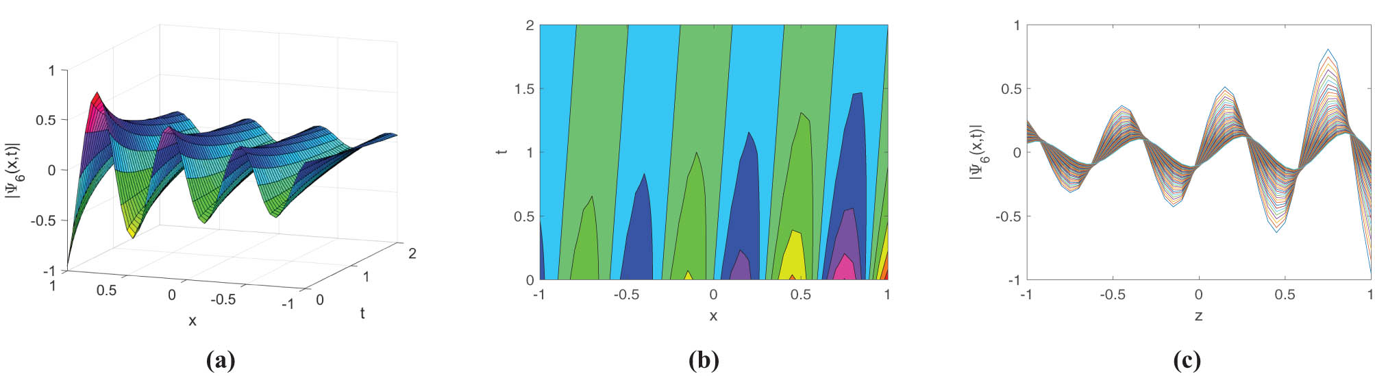
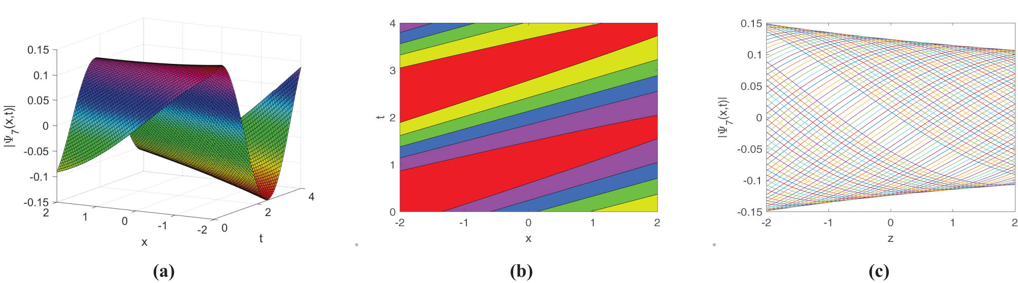
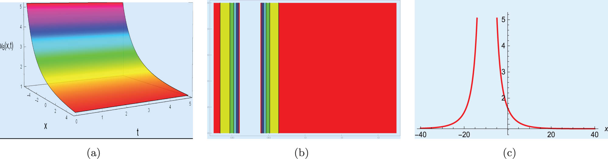
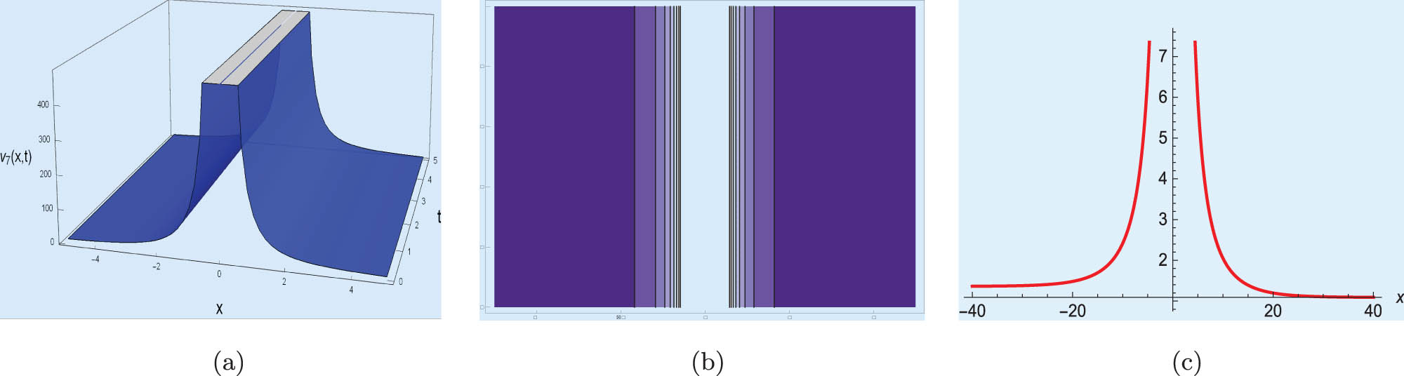
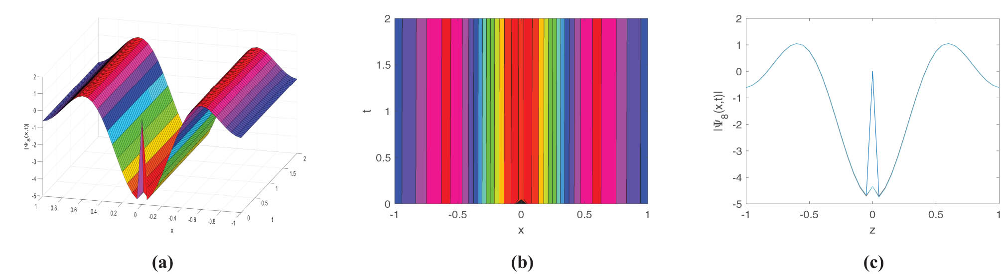
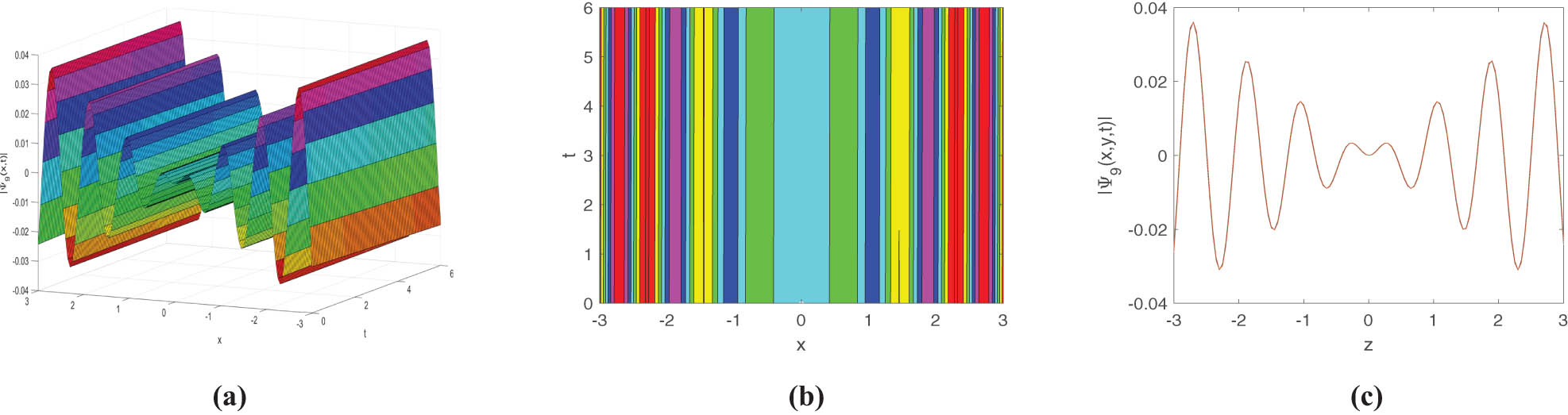
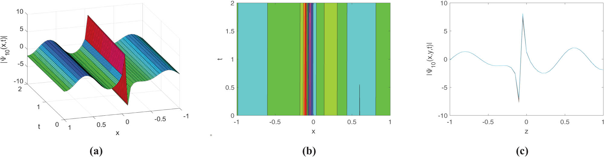
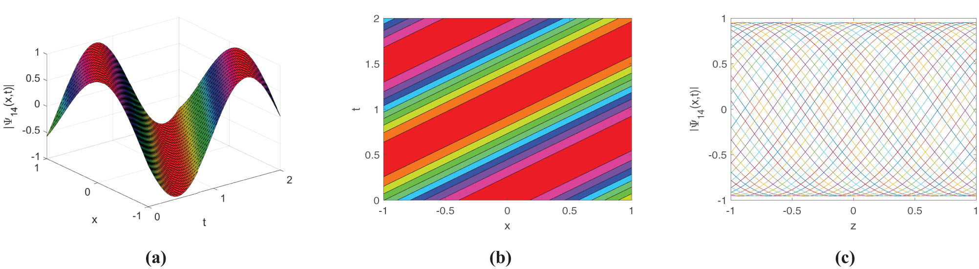
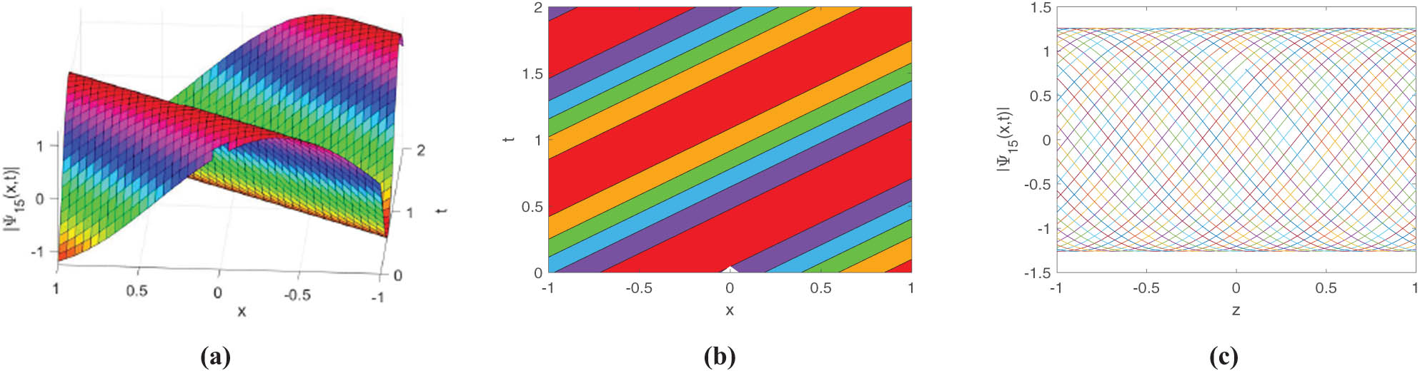
To demonstrate the physical Interpretation of the optical soliton solutions and to define the nature of optical solitons are illustrated through constructed 3D, contour, and 2D (line) graphs in this section. 2D and 3D plots are essential tools for visualizing and understanding the behavior of waves, particularly optical solitons, in various physical systems. The amplitude of the wave, such as height, pressure, or displacement, is usually plotted in two dimensions as a function of time or position. The wave’s shape, wavelength, and amplitude at a given time are revealed by a 2D plot of amplitude versus position. This offers the wave’s spatial profile. On the other hand, a 2D plot of amplitude versus time at a fixed position shows how the wave’s amplitude changes over time at that particular location, helping to observe the wave’s frequency and period. In the context of optical solitons, 2D plots can demonstrate the optical soliton’s characteristic shape and how it propagates without changing its form, such as a series of plots showing the optical soliton’s movement over time. These plots illustrate how the wave evolves through time and space and serve as useful tools for visualizing the behavior of optical solitons. The nature of optical soliton for different scenario is given below. Figures 1 and 2 present visual representations of dark optical soliton solutions. A dark optical soliton forms into waves that uphold their shape as they move through systems containing nonlinearity properties. Such waves appear because light intensity creates a reduction in the refractive index, which results in self-defocusing. Central light pulse spreading occurs as a result of dispersion, but it is offset by dispersion which makes different frequency components move at varying speeds. Self-defocusing interaction sustains dark optical solitons because it balances with the dispersion effects. Dark optical solitons show important characteristics such as a brightness dip in the middle of a brighter background alongside
Select
Select
Select
Select
Select for
Select for
Select for
Select
Select
Select
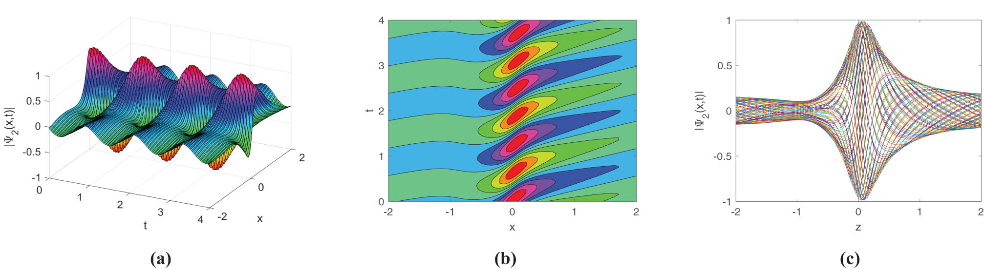
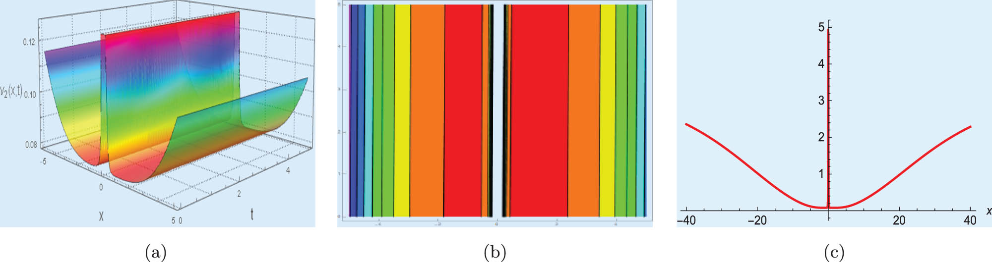
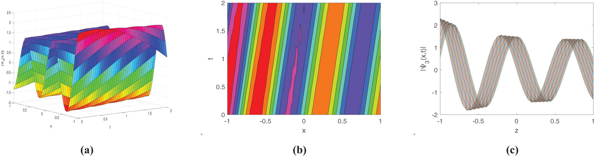
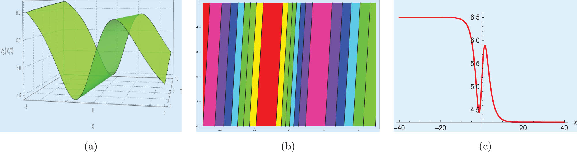
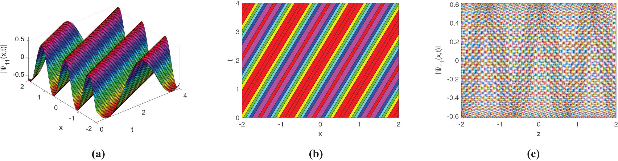
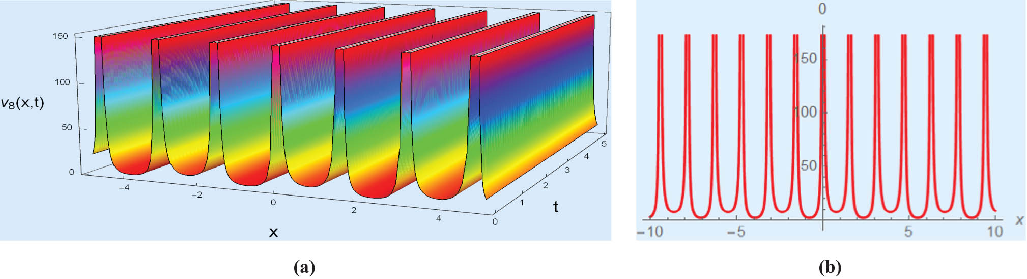
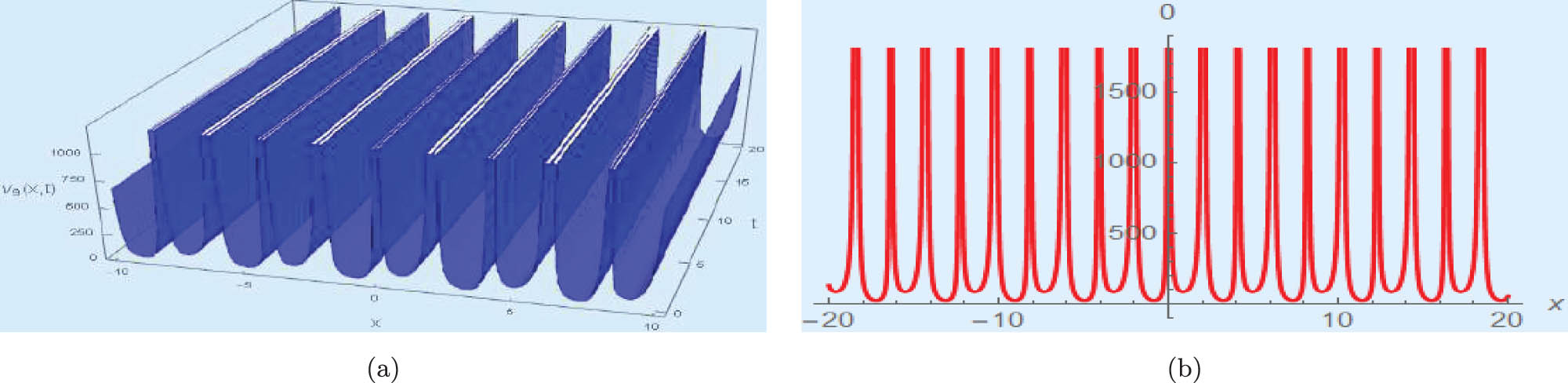
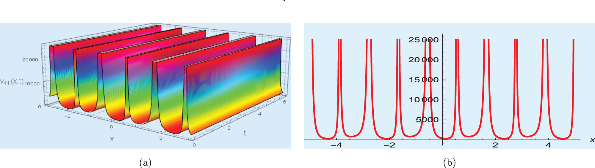
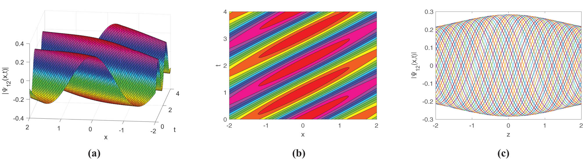
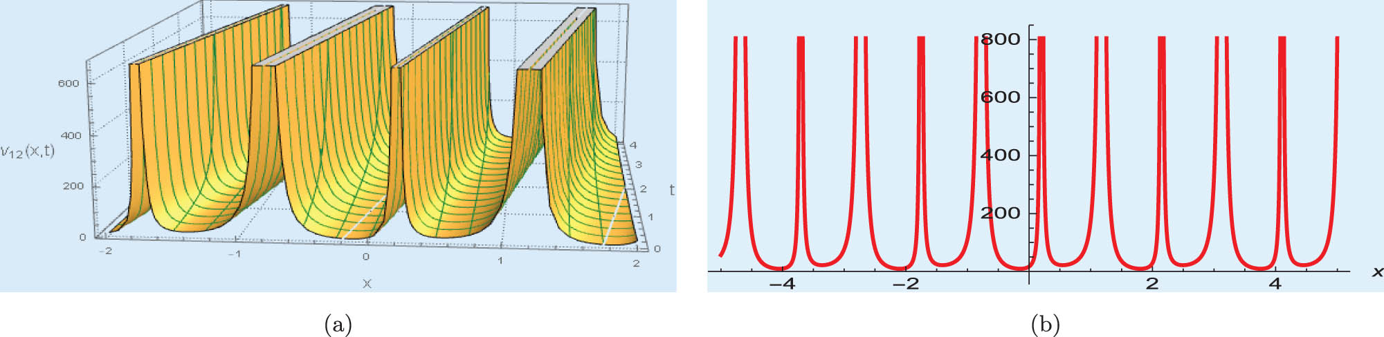
Dark-bright optical soliton appears together in Figures 11 and 12. The propagation of localized wave packets known as bright optical solitons fights against natural dispersion effects which cause wave spreading in time. Self-focusing develops through the balancing of dispersion in the medium and nonlinearity which either emerges from changes to refractive index due to intensity variations or from interatomic interactions. A stable localized wave packet emerges from this balanced state. The essential characteristics of bright optical solitons include elevated intensity above background levels together with shape preservation during transmission and resistance to external disturbances and interactions that handle them like particles. These localized waves exist in different systems, which include optical fibers used for distortion-free data transmission over long distances and Bose–Einstein condensates that produce localized matter waves through atomic interactions. Broad applications for bright optical solitons exist in fields of optical communications as well as laser technology and quantum computing and the study of nonlinear waves in fundamental research. Figures 13, 14, 15, 16, 17, 18, display singular periodic optical soliton solutions, and Figures 19, 20, 21, 22 display combination of singular periodic optical soliton solution. A periodic optical soliton refers to a optical soliton-like solution of a NLPDE that exhibits periodic behavior in space, time, or both. Unlike traditional optical solitons, which are localized and nonrepeating, periodic optical solitons are characterized by their repeating patterns while still retaining some optical soliton-like properties, such as stability and shape preservation during propagation. Periodic optical solitons arise in integrable systems and nonlinear wave equations, often as a result of balancing nonlinearity and dispersion. They are important in understanding wave phenomena in various physical systems, such as optics, fluid dynamics, and plasma physics.
Select
Select
Select
Select
Select
Select for
Select
Select
Select
Select
Select
Select
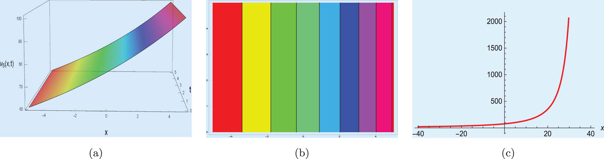
The rational form of optical soliton appears in Figure 23. A rational optical soliton stands as a type of optical soliton for NLPDEs when its solution takes the form of rational functions composed of ratios between polynomials. The decay pattern of standard optical solitons occurs exponentially while rational optical solitons use algebraic equations for their behavior
Select
5.2 Physical interpretation of bifurcation analysis results
Figure 24(a), the bifurcation diagram, plots the equilibrium values of
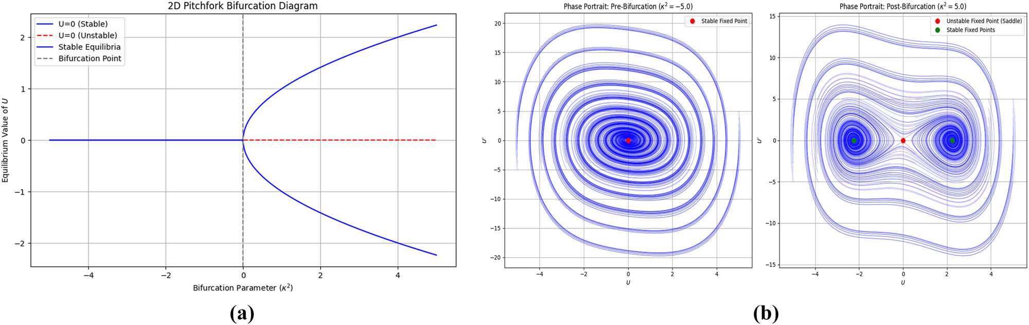
(a) A bifurcation diagram showing the equilibrium points of U as a function of the parameter ratio
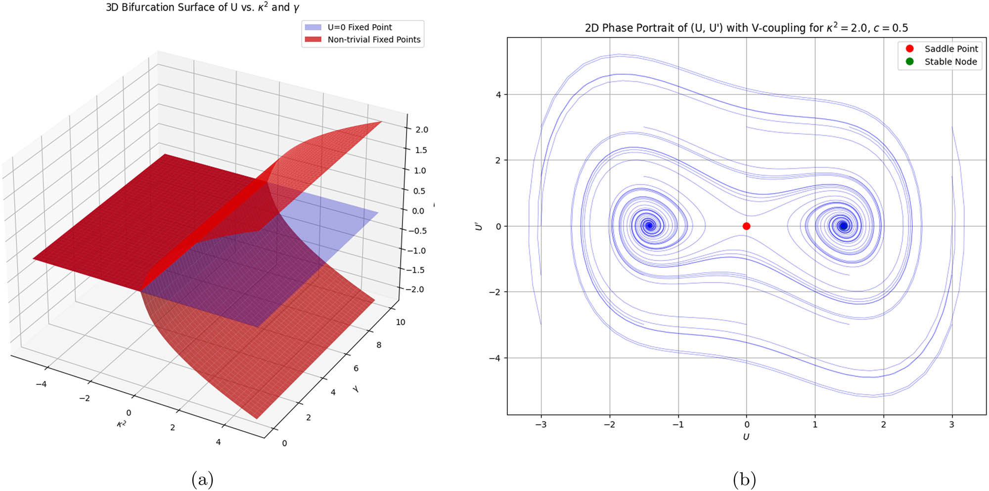
(a) A bifurcation diagram showing the equilibrium points of U as a function of the parameter ratio
6 Conclusion
This article demonstrated the successful application of the enhanced modified extended tanh-expansion method to construct optical soliton solutions of nonlinear Schrödinger–Bopp–Podolsky system. The nonlinear Schrödinger equation provides solid modeling capability for standard nonlinear media optical solitons yet struggles to handle complex optical systems adequately. The Bopp–Podolsky framework delivers advanced capabilities to study optical soliton stability alongside energy transport because it includes higher-order terms. The analytical findings prove that optical solitons keep their energy contained successfully, which establishes their critical role in optical communications technology. It has also been shown that the enhanced modified extended tanh-expansion method is adaptable and effective in handling nonlinear partial differential equations based on the solutions, which comprise optical solitons, periodic waves solutions, bright solutions, dark solutions, and singular solutions. The enhanced modified extended tanh-expansion method is compared to other methods such as
Acknowledgments
This research was financially supported by Firat University.
-
Funding information: The authors state no funding involved.
-
Author contributions: All authors have accepted responsibility for the entire content of this manuscript and approved its submission.
-
Conflict of interest: The authors state no conflict of interest.
-
Data availability statement: All data generated or analysed during this study are included in this published article.
References
[1] d’Avenia P, Siciliano G. Nonlinear Schrödinger equation in the Bopp-Podolsky electrodynamics: Solutions in the electrostatic case. J Differ Equ. 2019;267(2):1025–65. 10.1016/j.jde.2019.02.001Search in Google Scholar
[2] Li L, Pucci P, Tang X. Ground state solutions for the nonlinear Schrödinger–Bopp-Podolsky system with critical Sobolev exponent. Adv Nonlinear Stud. 2020;20(3):511–38. 10.1515/ans-2020-2097Search in Google Scholar
[3] Yang H, Yuan Y, Liu J. On Nonlinear Schrödinger–Bopp-Podolsky system with asymptotically periodic potentials. J Funct Spaces. 2022;2022:9287998. 10.1155/2022/9287998Search in Google Scholar
[4] Li Y, Ye H. Normalized solutions for Sobolev critical Schrödinger–Bopp-Podolsky systems. J Math Anal Appl. 2023;529(1):127569. 10.58997/ejde.2023.56Search in Google Scholar
[5] Jiang Q, Li L, Chen S, Siciliano G. Ground state solutions for the nonlinear Schrödinger–Bopp-Podolsky system with nonperiodic potentials. Electron J Differ Equ. 2024;2024:43–25. 10.58997/ejde.2024.43Search in Google Scholar
[6] Bahrouni A, Missaoui H. On the Schrödinger–Bopp-Podolsky system: Ground state & least energy nodal solutions with nonsmooth nonlinearity. 2022. arXiv: http://arXiv.org/abs/arXiv:2212.11389. Search in Google Scholar
[7] Hu Y, Wu X, Tang C. Existence of least-energy sign-changing solutions for the Schrödinger–Bopp-Podolsky system with critical growth. Bull Malays Math Sci Soc. 2023;46(1):45. 10.1007/s40840-022-01441-7Search in Google Scholar
[8] de Paula Ramos G. Cluster semiclassical states of the nonlinear Schrödinger–Bopp-Podolsky system. J Fixed Point Theory Appl. 2025;27(2):49. 10.1007/s11784-025-01198-zSearch in Google Scholar
[9] Liu J, Duan Y, Liao JF, Pan HL. Positive solutions for a non-autonomous Schrödinger–Bopp-Podolsky system. J Math Phys. 2023;64(10):101507. 10.1063/5.0159190Search in Google Scholar
[10] d’Avenia P, Siciliano G. Nonlinear Schrödinger equation in the Bopp-Podolsky electrodynamics: Global boundedness, blow-up and no scattering in the energy space. J Differ Equ. 2023;350:194–228. Search in Google Scholar
[11] Caponio E, d’Avenia P, Pomponio A, Siciliano G, Yang L. On a nonlinear Schrödinger–Bopp-Podolsky system in the zero mass case: functional framework and existence. 2025. arXiv: http://arXiv.org/abs/arXiv:2506.09752. Search in Google Scholar
[12] Santos Damian HM, Siciliano G. Schrödinger–Bopp-Podolsky system with sublinear and critical nonlinearities: solutions at negative energy levels and asymptotic behaviour. 2025. arXiv: http://arXiv.org/abs/arXiv:2507.19444. Search in Google Scholar
[13] Oliveira IG, Sales JH, Thibes R. Bopp-Podolsky scalar electrodynamics propagators and energy-momentum tensor in covariant and light-front coordinates. Eur Phys J Plus. 2020;135(9):1–13. Search in Google Scholar
[14] Oliveira IG, Sales JH, Thibes R. Bopp-Podolsky scalar electrodynamics propagators and energy-momentum tensor in covariant and light-front coordinates. 2020. arXiv e-prints, arXiv-2008. 10.1140/epjp/s13360-020-00733-wSearch in Google Scholar
[15] Gratus J, Perlick V, Tucker RW. On the self-force in Bopp-Podolsky electrodynamics. J Phys A Math Theor. 2015;48(43):435401. 10.1088/1751-8113/48/43/435401Search in Google Scholar
[16] Lazar M. Green functions and propagation in the Bopp-Podolsky electrodynamics. Wave Motion. 2019;91:102388. 10.1016/j.wavemoti.2019.102388Search in Google Scholar
[17] Siciliano G, Silva K. The fibering method approach for a non-linear Schrödinger equation coupled with the electromagnetic field. Bull Malays Math Sci Soc. 2023;46(1):45.Search in Google Scholar
[18] Chen S, Li L, Radulescu VD, Tang X. Ground state solutions of the non-autonomous Schrödinger Bopp Podolsky system. Anal Math Phys. 2022;12:1–32. 10.1007/s13324-021-00627-9Search in Google Scholar
[19] d’Avenia P, Ghimenti MG. Multiple solutions and profile description for a nonlinear Schrödinger Bopp Podolsky Proca system on a manifold. Calc Var Partial Differ Equ. 2022;61(6):223. 10.1007/s00526-022-02341-1Search in Google Scholar
[20] Afonso DG, Siciliano G. Normalized solutions to a Schrödinger Bopp Podolsky system under Neumann boundary conditions. Commun Contemp Math. 2021;15:2150100. 10.1142/S0219199721501005Search in Google Scholar
[21] Zheng P. Existence and finite time blow-up for nonlinear Schrödinger equations in the Bopp-Podolsky electrodynamics. J Math Anal Appl. 2022;514(2):126346. 10.1016/j.jmaa.2022.126346Search in Google Scholar
[22] Evans DJ, Raslan KR. The tanh function method for solving some important non-linear partial differential equations. Int J Comput Math. 2005;82(7):897–905. 10.1080/00207160412331336026Search in Google Scholar
[23] Heee JH, Wu XH. Exp-function method for nonlinear wave equations. Chaos Solitons Fractals. 2006;30(3):700–8. 10.1016/j.chaos.2006.03.020Search in Google Scholar
[24] Iqbal M, Seadawy AR, Lu D, Zhang Z. Structure of analytical and symbolic computational approach of multiple solitary wave solutions for nonlinear Zakharov-Kuznetsov modified equal width equation. Numer Methods Partial Differ Equ. 2023;39(5):3987–4006. 10.1002/num.23033Search in Google Scholar
[25] Iqbal M, Seadawy AR, Lu D, Zhang Z. Computational approach and dynamical analysis of multiple solitary wave solutions for nonlinear coupled Drinfeld-Sokolov-Wilson equation. Results Phys. 2023;54:107099. 10.1016/j.rinp.2023.107099Search in Google Scholar
[26] Iqbal M, Seadawy AR, Lu D, Zhang Z. Physical structure and multiple solitary wave solutions for the nonlinear Jaulent-Miodek hierarchy equation. Mod Phys Lett B. 2024;38(16):2341016. 10.1142/S0217984923410166Search in Google Scholar
[27] Iqbal M, Lu D, Seadawy AR, Alsubaie NE, Umurzakhova Z, Myrzakulov R. Dynamical analysis of exact optical soliton structures of the complex nonlinear Kuralay-II equation through computational simulation. Mod Phys Lett B. 2024;38(36):2450367. 10.1142/S0217984924503676Search in Google Scholar
[28] Iqbal M, Lu D, Seadawy AR, Zhang Z. Nonlinear behavior of dust acoustic periodic soliton structures of nonlinear damped modified Korteweg-de Vries equation in dusty plasma. Results Phys. 2024;59:107533. 10.1016/j.rinp.2024.107533Search in Google Scholar
[29] Iqbal M, Seadawy AR, Lu D, Zhang Z. Weakly restoring forces and shallow water waves with dynamical analysis of periodic singular solitons structures to the nonlinear Kadomtsev-Petviashvili-modified equal width equation. Mod Phys Lett B. 2024;38(27):2450265. 10.1142/S0217984924502658Search in Google Scholar
[30] Iqbal M, Lu D, Faridi WA, Murad MAS, Seadawy AR. A novel investigation on propagation of envelop optical soliton structure through a dispersive medium in the nonlinear Whitham-Broer-Kaup dynamical equation. Int J Theor Phys. 2024;63(5):131. 10.1007/s10773-024-05663-2Search in Google Scholar
[31] Iqbal M, Faridi WA, Ali R, Seadawy AR, Rajhi AA, Anqi AE, et al. Dynamical study of optical soliton structure to the nonlinear Landau-Ginzburg-Higgs equation through computational simulation. Opt Quantum Electron. 2024;56(7):1192. 10.1007/s11082-024-06401-ySearch in Google Scholar
[32] Manzoor Z, Iqbal MS, Hussain S, Ashraf F, Inc M, Akhtar Tarar M, et al. A study of propagation of the ultra-short femtosecond pulses in an optical fiber by using the extended generalized Riccati equation mapping method. Opt Quant Electron. 2023;55:717. 10.1007/s11082-023-04934-2Search in Google Scholar
[33] Chou D, Rehman HU, Haider R, Muhammad T, Li TL. Analyzing optical soliton propagation in perturbed nonlinear Schrödinger equation: a multi-technique study. Optik. 2024;302:171714. 10.1016/j.ijleo.2024.171714Search in Google Scholar
[34] Chou D, Boulaaras SM, Rehman HU, Iqbal I, Akram A, Ullah N. Additional investigation of the Biswas-Arshed equation to reveal optical soliton dynamics in birefringent fiber. Opt Quantum Electron. 2024;56(4):705. 10.1007/s11082-024-06366-ySearch in Google Scholar
[35] Chou D, UrRehman H, Amer A, Amer A. New solitary wave solutions of generalized fractional Tzitzéica-type evolution equations using Sardar sub-equation method. Opt Quantum Electron. 2023;55(13):1148. 10.1007/s11082-023-05425-0Search in Google Scholar
[36] Chou D, Boulaaras SM, Rehman HU, Iqbal I. Probing wave dynamics in the modified fractional nonlinear Schrödinger equation: implications for ocean engineering. Opt Quantum Electron. 2024;56(2):228. 10.1007/s11082-023-05954-8Search in Google Scholar
[37] Fahad A, Boulaaras SM, Rehman HU, Iqbal I, Saleem MS, Chou D. Analysing soliton dynamics and a comparative study of fractional derivatives in the nonlinear fractional Kudryashovas equation. Results Phys. 2023;55:107114. 10.1016/j.rinp.2023.107114Search in Google Scholar
[38] Esen H, Ozisik M, Secer A, Bayram M. Optical soliton perturbation with Fokas Lenells equation via enhanced modified extended tanh-expansion approach. Optik. 2022;267:169615. 10.1016/j.ijleo.2022.169615Search in Google Scholar
[39] Ashraf R, Ashraf F, Akguel A, Ashraf S, Alshahrani B, Mahmoud M, et al. Some new soliton solutions to the (3+1)-dimensional generalized KdV-ZK equation via enhanced modified extended tanh-expansion approach. Alexandria Eng J. 2023;69:303–9. 10.1016/j.aej.2023.01.007Search in Google Scholar
[40] Alam LMB, Jiang X. Exact and explicit traveling wave solution to the time-fractional phi-four and (2+1) dimensional CBS equations using the modified extended tanh-function method in mathematical physics. Partial Differ Equ Appl Math. 2021;4:100039. 10.1016/j.padiff.2021.100039Search in Google Scholar
[41] Ananna SN, Gharami PP, An T, Asaduzzaman M. The improved modified extended tanh-function method to develop the exact travelling wave solutions of a family of 3D fractional WBBM equations. Results Phys. 2022;41:105969. 10.1016/j.rinp.2022.105969Search in Google Scholar
[42] Ozdemir N, Secer A, Ozisik M, Bayram M. Perturbation of dispersive optical solitons with Schrödinger-Hirota equation with Kerr law and spatio-temporal dispersion. Optik. 2022;265:169545. 10.1016/j.ijleo.2022.169545Search in Google Scholar
[43] Samir I, Badra N, Ahmed HM, Arnous AH. Optical soliton perturbation with Kudryashovas generalized law of refractive index and generalized nonlocal laws by improved modified extended tanh method. Alexandria Eng J. 2022;61(5):3365–74. 10.1016/j.aej.2021.08.050Search in Google Scholar
[44] Refaie Ali A, Alam MN, Parven MW. Unveiling optical soliton solutions and bifurcation analysis in the space-time fractional Fokas-Lenells equation via SSE approach. Sci Rep. 2024;14(1):2000. 10.1038/s41598-024-52308-9Search in Google Scholar PubMed PubMed Central
[45] Alam MN, Iqbal M, Hassan M, Fayz-Al-Asad M, Hossain MS, Tunç C. Bifurcation, phase plane analysis and exact soliton solutions in the nonlinear Schrodinger equation with Atanganaas conformable derivative. Chaos Solitons Fractals. 2024;182:114724. 10.1016/j.chaos.2024.114724Search in Google Scholar
[46] Iqbal I, Boulaaras SM, Althobaiti S, Althobaiti A, Rehman HU. Exploring soliton dynamics in the nonlinear Helmholtz equation: bifurcation, chaotic behavior, multistability, and sensitivity analysis. Nonlinear Dyn. 2025;113(13):16933–54. 10.1007/s11071-025-10961-3Search in Google Scholar
© 2025 the author(s), published by De Gruyter
This work is licensed under the Creative Commons Attribution 4.0 International License.
Articles in the same Issue
- Research Articles
- Generalized (ψ,φ)-contraction to investigate Volterra integral inclusions and fractal fractional PDEs in super-metric space with numerical experiments
- Solitons in ultrasound imaging: Exploring applications and enhancements via the Westervelt equation
- Stochastic improved Simpson for solving nonlinear fractional-order systems using product integration rules
- Exploring dynamical features like bifurcation assessment, sensitivity visualization, and solitary wave solutions of the integrable Akbota equation
- Research on surface defect detection method and optimization of paper-plastic composite bag based on improved combined segmentation algorithm
- Impact the sulphur content in Iraqi crude oil on the mechanical properties and corrosion behaviour of carbon steel in various types of API 5L pipelines and ASTM 106 grade B
- Unravelling quiescent optical solitons: An exploration of the complex Ginzburg–Landau equation with nonlinear chromatic dispersion and self-phase modulation
- Perturbation-iteration approach for fractional-order logistic differential equations
- Variational formulations for the Euler and Navier–Stokes systems in fluid mechanics and related models
- Rotor response to unbalanced load and system performance considering variable bearing profile
- DeepFowl: Disease prediction from chicken excreta images using deep learning
- Channel flow of Ellis fluid due to cilia motion
- A case study of fractional-order varicella virus model to nonlinear dynamics strategy for control and prevalence
- Multi-point estimation weldment recognition and estimation of pose with data-driven robotics design
- Analysis of Hall current and nonuniform heating effects on magneto-convection between vertically aligned plates under the influence of electric and magnetic fields
- A comparative study on residual power series method and differential transform method through the time-fractional telegraph equation
- Insights from the nonlinear Schrödinger–Hirota equation with chromatic dispersion: Dynamics in fiber–optic communication
- Mathematical analysis of Jeffrey ferrofluid on stretching surface with the Darcy–Forchheimer model
- Exploring the interaction between lump, stripe and double-stripe, and periodic wave solutions of the Konopelchenko–Dubrovsky–Kaup–Kupershmidt system
- Computational investigation of tuberculosis and HIV/AIDS co-infection in fuzzy environment
- Signature verification by geometry and image processing
- Theoretical and numerical approach for quantifying sensitivity to system parameters of nonlinear systems
- Chaotic behaviors, stability, and solitary wave propagations of M-fractional LWE equation in magneto-electro-elastic circular rod
- Dynamic analysis and optimization of syphilis spread: Simulations, integrating treatment and public health interventions
- Visco-thermoelastic rectangular plate under uniform loading: A study of deflection
- Threshold dynamics and optimal control of an epidemiological smoking model
- Numerical computational model for an unsteady hybrid nanofluid flow in a porous medium past an MHD rotating sheet
- Regression prediction model of fabric brightness based on light and shadow reconstruction of layered images
- Dynamics and prevention of gemini virus infection in red chili crops studied with generalized fractional operator: Analysis and modeling
- Qualitative analysis on existence and stability of nonlinear fractional dynamic equations on time scales
- Fractional-order super-twisting sliding mode active disturbance rejection control for electro-hydraulic position servo systems
- Analytical exploration and parametric insights into optical solitons in magneto-optic waveguides: Advances in nonlinear dynamics for applied sciences
- Bifurcation dynamics and optical soliton structures in the nonlinear Schrödinger–Bopp–Podolsky system
- User profiling in university libraries by combining multi-perspective clustering algorithm and reader behavior analysis
- Exploring bifurcation and chaos control in a discrete-time Lotka–Volterra model framework for COVID-19 modeling
- Review Article
- Haar wavelet collocation method for existence and numerical solutions of fourth-order integro-differential equations with bounded coefficients
- Special Issue: Nonlinear Analysis and Design of Communication Networks for IoT Applications - Part II
- Silicon-based all-optical wavelength converter for on-chip optical interconnection
- Research on a path-tracking control system of unmanned rollers based on an optimization algorithm and real-time feedback
- Analysis of the sports action recognition model based on the LSTM recurrent neural network
- Industrial robot trajectory error compensation based on enhanced transfer convolutional neural networks
- Research on IoT network performance prediction model of power grid warehouse based on nonlinear GA-BP neural network
- Interactive recommendation of social network communication between cities based on GNN and user preferences
- Application of improved P-BEM in time varying channel prediction in 5G high-speed mobile communication system
- Construction of a BIM smart building collaborative design model combining the Internet of Things
- Optimizing malicious website prediction: An advanced XGBoost-based machine learning model
- Economic operation analysis of the power grid combining communication network and distributed optimization algorithm
- Sports video temporal action detection technology based on an improved MSST algorithm
- Internet of things data security and privacy protection based on improved federated learning
- Enterprise power emission reduction technology based on the LSTM–SVM model
- Construction of multi-style face models based on artistic image generation algorithms
- Research and application of interactive digital twin monitoring system for photovoltaic power station based on global perception
- Special Issue: Decision and Control in Nonlinear Systems - Part II
- Animation video frame prediction based on ConvGRU fine-grained synthesis flow
- Application of GGNN inference propagation model for martial art intensity evaluation
- Benefit evaluation of building energy-saving renovation projects based on BWM weighting method
- Deep neural network application in real-time economic dispatch and frequency control of microgrids
- Real-time force/position control of soft growing robots: A data-driven model predictive approach
- Mechanical product design and manufacturing system based on CNN and server optimization algorithm
- Application of finite element analysis in the formal analysis of ancient architectural plaque section
- Research on territorial spatial planning based on data mining and geographic information visualization
- Fault diagnosis of agricultural sprinkler irrigation machinery equipment based on machine vision
- Closure technology of large span steel truss arch bridge with temporarily fixed edge supports
- Intelligent accounting question-answering robot based on a large language model and knowledge graph
- Analysis of manufacturing and retailer blockchain decision based on resource recyclability
- Flexible manufacturing workshop mechanical processing and product scheduling algorithm based on MES
- Exploration of indoor environment perception and design model based on virtual reality technology
- Tennis automatic ball-picking robot based on image object detection and positioning technology
- A new CNN deep learning model for computer-intelligent color matching
- Design of AR-based general computer technology experiment demonstration platform
- Indoor environment monitoring method based on the fusion of audio recognition and video patrol features
- Health condition prediction method of the computer numerical control machine tool parts by ensembling digital twins and improved LSTM networks
- Establishment of a green degree evaluation model for wall materials based on lifecycle
- Quantitative evaluation of college music teaching pronunciation based on nonlinear feature extraction
- Multi-index nonlinear robust virtual synchronous generator control method for microgrid inverters
- Manufacturing engineering production line scheduling management technology integrating availability constraints and heuristic rules
- Analysis of digital intelligent financial audit system based on improved BiLSTM neural network
- Attention community discovery model applied to complex network information analysis
- A neural collaborative filtering recommendation algorithm based on attention mechanism and contrastive learning
- Rehabilitation training method for motor dysfunction based on video stream matching
- Research on façade design for cold-region buildings based on artificial neural networks and parametric modeling techniques
- Intelligent implementation of muscle strain identification algorithm in Mi health exercise induced waist muscle strain
- Optimization design of urban rainwater and flood drainage system based on SWMM
- Improved GA for construction progress and cost management in construction projects
- Evaluation and prediction of SVM parameters in engineering cost based on random forest hybrid optimization
- Museum intelligent warning system based on wireless data module
- Optimization design and research of mechatronics based on torque motor control algorithm
- Special Issue: Nonlinear Engineering’s significance in Materials Science
- Experimental research on the degradation of chemical industrial wastewater by combined hydrodynamic cavitation based on nonlinear dynamic model
- Study on low-cycle fatigue life of nickel-based superalloy GH4586 at various temperatures
- Some results of solutions to neutral stochastic functional operator-differential equations
- Ultrasonic cavitation did not occur in high-pressure CO2 liquid
- Research on the performance of a novel type of cemented filler material for coal mine opening and filling
- Testing of recycled fine aggregate concrete’s mechanical properties using recycled fine aggregate concrete and research on technology for highway construction
- A modified fuzzy TOPSIS approach for the condition assessment of existing bridges
- Nonlinear structural and vibration analysis of straddle monorail pantograph under random excitations
- Achieving high efficiency and stability in blue OLEDs: Role of wide-gap hosts and emitter interactions
- Construction of teaching quality evaluation model of online dance teaching course based on improved PSO-BPNN
- Enhanced electrical conductivity and electromagnetic shielding properties of multi-component polymer/graphite nanocomposites prepared by solid-state shear milling
- Optimization of thermal characteristics of buried composite phase-change energy storage walls based on nonlinear engineering methods
- A higher-performance big data-based movie recommendation system
- Nonlinear impact of minimum wage on labor employment in China
- Nonlinear comprehensive evaluation method based on information entropy and discrimination optimization
- Application of numerical calculation methods in stability analysis of pile foundation under complex foundation conditions
- Research on the contribution of shale gas development and utilization in Sichuan Province to carbon peak based on the PSA process
- Characteristics of tight oil reservoirs and their impact on seepage flow from a nonlinear engineering perspective
- Nonlinear deformation decomposition and mode identification of plane structures via orthogonal theory
- Numerical simulation of damage mechanism in rock with cracks impacted by self-excited pulsed jet based on SPH-FEM coupling method: The perspective of nonlinear engineering and materials science
- Cross-scale modeling and collaborative optimization of ethanol-catalyzed coupling to produce C4 olefins: Nonlinear modeling and collaborative optimization strategies
- Unequal width T-node stress concentration factor analysis of stiffened rectangular steel pipe concrete
- Special Issue: Advances in Nonlinear Dynamics and Control
- Development of a cognitive blood glucose–insulin control strategy design for a nonlinear diabetic patient model
- Big data-based optimized model of building design in the context of rural revitalization
- Multi-UAV assisted air-to-ground data collection for ground sensors with unknown positions
- Design of urban and rural elderly care public areas integrating person-environment fit theory
- Application of lossless signal transmission technology in piano timbre recognition
- Application of improved GA in optimizing rural tourism routes
- Architectural animation generation system based on AL-GAN algorithm
- Advanced sentiment analysis in online shopping: Implementing LSTM models analyzing E-commerce user sentiments
- Intelligent recommendation algorithm for piano tracks based on the CNN model
- Visualization of large-scale user association feature data based on a nonlinear dimensionality reduction method
- Low-carbon economic optimization of microgrid clusters based on an energy interaction operation strategy
- Optimization effect of video data extraction and search based on Faster-RCNN hybrid model on intelligent information systems
- Construction of image segmentation system combining TC and swarm intelligence algorithm
- Particle swarm optimization and fuzzy C-means clustering algorithm for the adhesive layer defect detection
- Optimization of student learning status by instructional intervention decision-making techniques incorporating reinforcement learning
- Fuzzy model-based stabilization control and state estimation of nonlinear systems
- Optimization of distribution network scheduling based on BA and photovoltaic uncertainty
- Tai Chi movement segmentation and recognition on the grounds of multi-sensor data fusion and the DBSCAN algorithm
- Special Issue: Dynamic Engineering and Control Methods for the Nonlinear Systems - Part III
- Generalized numerical RKM method for solving sixth-order fractional partial differential equations