Fuzzy model-based stabilization control and state estimation of nonlinear systems

3.1 Sedation control of nonlinear time-varying time-lag systems based on the T-S fuzzy model

The T-S fuzzy model treats the dynamical NS as a weighted sum of some linear subsystems. The divided subsystems will be used to represent the characteristics of each part of NS [18]. The T-S fuzzy model is used to represent a nonlinear time-varying time-lag system. Eq. (1) provides the fuzzy rule.

In Eq. (1), r is the quantity of fuzzy rules. t represents a certain moment in time. x ( t ) is the state vector. x ̇ is the derivative of the state vector x ( t ) , representing the dynamic rate of change of the system at time t . ϕ represents the initial state function within the interval t ∈ [ − τ , 0 ] . It provides the system’s state history within the initial time window to calculate the impact of time delay. μ ( t ) is the control input vector. A i , A d i , and B i serve as known matrices of system parameters with appropriate dimensions. ξ p ( t ) is the antecedent variable. N i p is the fuzzy set. d ( t ) is the time-varying time lag of the system. However, in practice, many complex control systems are affected by certain delay phenomena. This delay usually has a significantly negative impact on control effectiveness. In severe cases, it can cause instability in the power system. To enhance the stability, a new time-delay-related Lyapunov asymptotic stability criterion is introduced. That is, for a positive definite number, a sufficient condition for a T-S fuzzy time-varying time-lag system to gradually stabilize at u(t) = 0 is the existence of a symmetric positive definite matrix, such that the linear matrix inequality holds. The corresponding linear matrix inequality (LMI) is given in the following equation:

In Eq. (2), W denotes a symmetric positive definite matrix and S i j denotes an arbitrary matrix. The criterion uses an auxiliary integral inequality, combined with inverse convexity, to define the differential equations of the generalized function, thus reducing the conservativeness of the obtained delay-related asymptotic stability criterion. On this basis, appropriate additional functions are selected, and the additional functions are transformed into other integral inequalities such as Jensen and Wirtinger [19]. The research intends to introduce the affiliation function from type II fuzzy mathematics into fuzzy mathematics with fuzzy properties to characterize various uncertainties. Eq. (3) is its mathematical representation.

In Eq. (3), the type II fuzzy set A ˜ is represented by a combination of a master-subordinate variable u ( x ) and a subordinate variable μ A ˜ ( x , u ( x ) ) . The subordinate variable is 1 in an interval, so that the subordinate variable can be avoided, which greatly reduces the complexity of the solution. The master-slave function with a mean uncertainty of Gaussian affiliation is selected. m represents the mean parameter, which appears in Gaussian membership functions and represents the center point of the distribution. x represents a state variable, indicating the current state or condition of the system. m 1 and m 2 denote the upper and lower bounds of the mean change, respectively. σ is the dispersion. In the fuzzy set recognition process, only the three parameters mentioned above need to be selected to obtain the parameters of the fuzzy set. D is the sample dataset. J x is the set of main affiliation function. Figure 1 shows the structure of the type II fuzzy model.

Figure 1

Structure diagram of a type II fuzzy model.

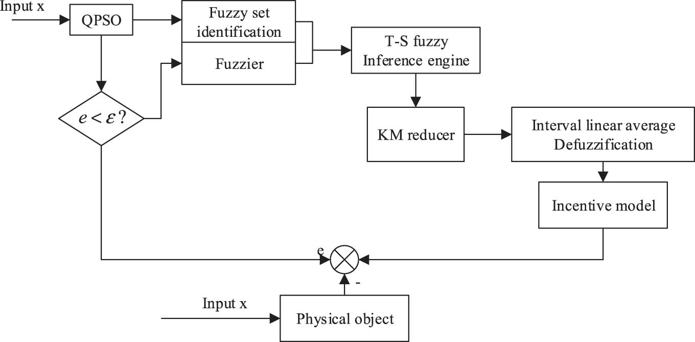
The model carries out self-adjustment based on the error feedback logic. Due to the time efficiency of the model correction, the offline parameter library is updated when the deviation exceeds the set threshold, and the fuzzy link is adaptively corrected when the deviation exceeds the set threshold. If the error of the method is within the given threshold, the accuracy of the method can be judged.

3.2 Dynamic state estimation based on the UKF algorithm

The Kalman filtering algorithm treats the signal generation process as the output of a pure linear system under Gaussian white noise and uses a state equation to describe this input–output relationship. This process involves the system state equation, observation equation, and white noise excitation, and its statistical characteristics form a recursive filtering algorithm. Figure 2 shows the schematic diagram of the Kalman filter algorithm.

Figure 2

Schematic diagram of the Kalman filter algorithm.

The UKF uses a method based on unscented transformation to solve nonlinear modeling problems. The so-called “unscented transformation” refers to constructing a series of point sets (collectively called sigma points) with the same mean and variance as the random variables and introducing them into a nonlinear generalized function to obtain a new generalized function. Eq. (4) is the algebraic equation.

In Eq. (4), x ′ , y , and u serve as the state variables, measurement variables, and input variables, respectively. f c is the nonlinear function of state variables. h c denotes the nonlinear function of measurement equations. ω and υ are the process noise and measurement noise, respectively. To address the interference of non-Gaussian measurement noise and outliers on the system dynamics state, a new robust cost function, extended kernel risk sensitive loss (EKRSL), is proposed to improve the suppression ability, whose expression is shown in the following equation:

In Eq. (5), E is the mathematical expectation. λ is the risk-sensitive parameter. κ σ is represented as a Gaussian kernel function with a kernel width of σ . When the desired object is only κ σ , the loss function becomes a mutual correlation entropy loss. This loss function is usually used to measure the comparability of expectations and responses. However, due to its non-convexity, the optimal solution of the method has a sharp gradient that changes flatly when the difference is too large. The study uses a generalized Gaussian density function to further reduce the effect of non-Gaussian noise and outliers. The generalized Gaussian density function is shown in the following equation:

In Eq. (6), Γ is the gamma function. p is the exponential term used to adjust the decay rate. β = 2 σ represents the kernel parameter.

3.3 Joint state estimation based on deep residual networks

This study develops a model-based NS state prediction method that uses machine learning methods for online prediction. Machine learning technology can learn knowledge from a large amount of real information and use available information to predict and evaluate systems. Deep learning has universality. Therefore, the study suggests developing a data assimilation model suitable for complex models, especially those with high accuracy and precise observations. Figure 3 shows a schematic diagram of the residual network architecture.

Figure 3

Schematic diagram of residual network architecture.

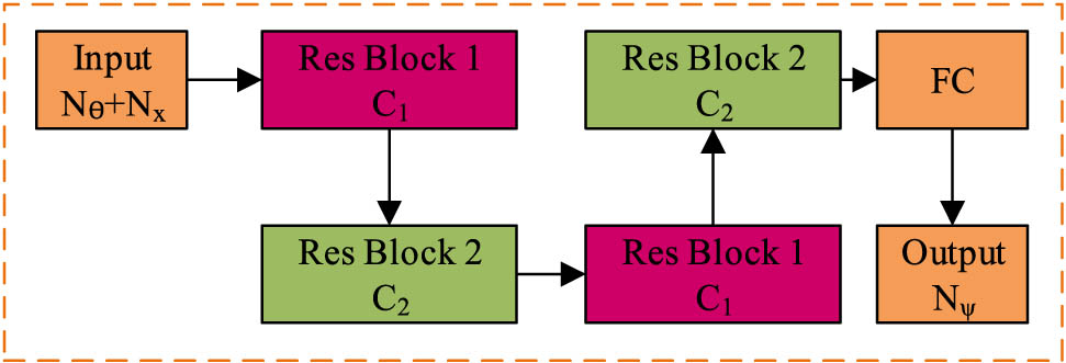
The deep residual network achieves “vector-vector” regression fitting. In this network, each convolutional body contains three sequential components, namely a two-dimensional convolutional layer, a normalization layer, and a modified linear excitation layer. The residual network structure is shown in Figure 4.

Figure 4

Network module diagrams. (a) Residual block 1. (b) Residual block 2.

The overall construction of this residual network is two different residual modalities which are built on different levels and pass the information obtained on the previous level to the next level [20]. Eq. (7) is the mathematical expression of the agent model.

In Eq. (7), both X k a and X k b denote state values and ψ DL denotes the nonlinear mapping. To effectively find the optimal parameters, the attention mechanism and DropBlock layer are introduced to optimize the deep residual network. Figure 5 shows a schematic diagram of the attention unit structure.

Figure 5

Schematic diagram of the attention unit structure.

The attention mechanism contains two aspects, i.e., compression and excitation. The method uses compression and excitation modules to automatically adjust the weights of each feature pathway, which in turn reinforces the weights of each feature pathway and suppresses the redundant features. To regulate the weighting relationship between channels, it is necessary to compress the feature information in the channels and transform the input W × H × C feature information into the input of 1 × 1 × C using the pooling layer. The global information expression of the feature map is shown in the following equation:

In Eq. (8), z c is the feature output. F sq is the squeezing operation. u c is the feature input. ( i , j ) serves as the coordinate re-excitation operation of the feature, which associates the overall data obtained in the previous step with a fully connected layer of dimension C ÷ r × C . C ÷ r × C is used as a scale parameter, which serves to reduce the number of channels, the number of parameters, and the computational complexity. It is restarted and transmitted to the next fully connected layer, restoring all the number of channels. The role of the two fully connected layer is to combine the signals extracted from each channel. Then, the sigmoid function is used to transform the input of each channel to obtain the weighted value of each channel, as shown in the following equation:

In Eq. (9), s is the channel weight parameter. F ex is the excitation operation. W 1 and W 2 are fully connected layers. σ is the ReLU function. DropBlock is a regularization algorithm that sets the size of each block cell to obtain more robust properties and can be used at the convolutional layer and at the entire connected layer. Eq. (10) is its mathematical representation.

In Eq. (10), ρ denotes the probability that the activation cell remains active. f s 2 denotes the size of the feature. s denotes the size of the square of the drop. γ denotes the number of square activation cells of the drop.

4.1 Example analysis of stabilization control model based on an improved T-S fuzzy model

To verify the effectiveness of the improved T-S fuzzy model used in the study for NSs, two examples are analyzed. Example one analyzes the angular and positional state response of the truck-trailer system, taking the initial state of this truck-trailer system as x ( 0 ) = ( 0.5 π 0 .75π − 5 ) T and the time-varying time lag of the system as d ( t ) = 5 + 5 sin ( 0.04 t ) . Example two analyzes the temperature difference (TD) output results for the air preheater mechanism model with the input μ values taken as 0.2, 0.4, and 0.6. Table 1 shows the maximum time-delay allowed upper bound obtained under different conditions.

Table 1 illustrates that the maximum time-delay allowed upper bound obtained from the fuzzy model in the study is at the highest value, regardless of the input μ. The maximum time-delay that the system can maintain stability is higher than other models. For example, when μ is 0.2, the maximum time-delay allowed upper bound is 2.1123, while the maximum time-delay allowed upper bound for the extended affine T-S fuzzy system and the improved T-S fuzzy system with free matrix are 1.5389 and 1.6785, respectively. The model is 0.5734 and 0.4338 higher, respectively. This indicates that the model is more superior in stability determination. Figure 6 shows the results of each status response of the trailer.

Figure 6

Trailer status responses. (a) Angular deviation curve. (b) Horizontal deviation curve. (c) Vertical deviation curve.

In Figure 6(a), in the angular deviation response, the proposed improved T-S fuzzy model as well as the type II affiliation function decreases from the starting value of 1.8°, drops to −0.01° after 3 s, and then climbs to 0° after 2 s, and starts to converge at this point. The curve level does not fluctuate, and the convergence performance is good in the middle and latter stages. While the adaptive fuzzy model starts with the same value as the proposed model, at 1.8°, and then the curve drops below 0°. However, the whole curve is in a fluctuating state, with a sawtooth shape and a fluctuation range of ±0.5°, and the angle control is unstable. The fuzzy model has good control effect on angle calming. Figure 6(b) and (c) shows that the initial values of the horizontal displacement deviation state response and vertical displacement deviation state response of the proposed model are 4.6 and 1.3, respectively. Afterward, the curves show a rapid decline followed by a slow rise, with the lowest values of both curves around −0.4°. The initial convergence time is 4 s, and the curves then show a stable convergence state with a convergence value of 0. The adaptive fuzzy model does not show a convergence trend in the middle and later states and oscillates frequently, with the oscillation range between ±0.4. In contrast, the proposed model possesses higher control accuracy and stability in the displacement deviation in both directions. Figure 7 shows the TD calming curve.

Figure 7

TD curve output results. (a) Comparison of temperature difference at the outlet of secondary air. (b) Comparison of flue gas outlet temperature difference.

In Figure 7(a), on the TD of secondary air outlet, the TD curve of the proposed fuzzy model is relatively more volatile in the first period from 10 to 25 s, with the fluctuation range between −10 and 10 K. The fluctuation starts to decrease in the latter period, with the fluctuation range between −5 and −2 K. When between 25 and 52 s, the TD curve is in the best stage, with the smallest fluctuation, and can stable around 0. The TD curve of the adaptive fuzzy model starts from a higher value of 30 K and drops to within ±10 K within 18 s. The curve fluctuates around −10 K. At 26 s, it then rises to 10 K, lasts for 25 s, and then climbs again at the back end of the curve, with TD exceeding 10 K. The results indicate that the proposed model achieves superior TD control compared with comparison methods. From Figure 7(b), in the flue gas outlet, the starting value of the proposed fuzzy control model is 9 K, and the curve drops to −20 K around 20 s, with an increase in negative deviation. At 30 s, the curve climbs above 0 again with an error of 10 K, and then the TD curve remains around 0 with fluctuations not exceeding 5 K. The flue gas temperature error curve of the adaptive fuzzy model not only has an initial value higher than 60 K but also the overall curve is located above the curve of the proposed model, with most curve segments higher than 20 K, resulting in significant errors and inability to achieve better control performance. Table 2 shows the error index results.

From Table 2, the MAE reflects an average error. The output error of the modified T-S fuzzy model based on the proposed method is smaller compared with the simplified fixed-service mechanism model. The adaptive fuzzy model MAPD can reflect the error in a way that reduces the impact of outliers on the error indicator under fast variable load conditions. The comparison shows that the MAPD obtained based on the modified T-S fuzzy model is much smaller than that obtained from the adaptive fuzzy model and the 800 MW constant operating condition process, which proves that this model is better in handling parameter uncertainty. In addition, the modified T-S fuzzy mathematical method on the air preheater can better simulate the dynamic changes of various parameters under variable load conditions, with higher accuracy.

4.2 Example analysis of a state estimation model based on an improved UKF

The effectiveness of the improved UKF is tested under various complex noise disturbances using 68 typical arithmetic cases from 16 machines. Real data are added to the measurement vector and input vector, which contain the voltage, current, active power, and reactive power on the terminal bus of each generator. In addition, given that real-life noise is non-Gaussian distributed in a statistical sense, the study proposes obtaining statistically significant heterogeneous noise by iterating voltage vectors to obtain outliers and further investigate the effect of outliers on the method. Figure 8 shows the state estimation results for each algorithm under Gaussian measurement noise.

Figure 8

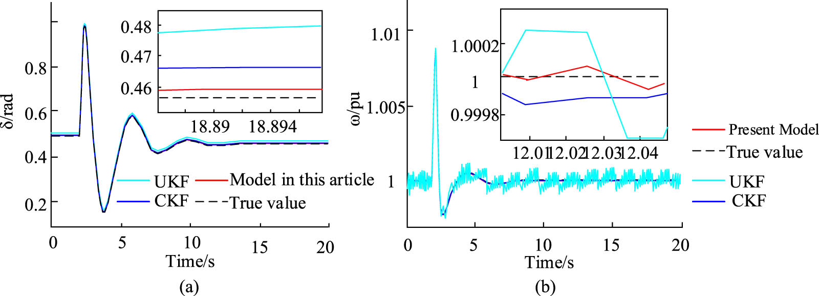
State estimation results of various algorithms under Gaussian measurement noise. (a) Phase angle. (b) Angular frequency.

In Figure 8, the phase angle curves corresponding to the three Kalman filtering methods all show a similar trend to the actual phase angle curve, that is, they first experience an oscillation period and then tend to converge. The oscillation frequency is three times, and the oscillation amplitude decreases from 0.98 at the peak to 0.46 at the peak. The entire oscillation time is 10 s, and the curve begins to converge after 10 s. However, the error between the proposed improved UKF state estimation model and the actual convergence value is the smallest, with an error of 0.1%. The error of UKF and cubature Kalman filter (CKF) was 4.3 and 1.7%, respectively. Similarly, the state estimation model used in the study achieves the highest accuracy within 0.0001 in estimating the system angular frequency parameters. The accuracy of the UKF and CKF state estimation models is 0.0025 and 0.0017, respectively. The model has better performance in estimating the true value. Figure 9 shows the state estimation results with outliers.

Figure 9

State estimation results of different algorithms with outlier in measurement noise. (a) Phase angle. (b) Angular frequency.

In Figure 9, as outliers are added to the mixed non-Gaussian noise, the parameter estimation performance of UFK significantly decreases, and its corresponding phase angle curve exhibits more fluctuations in the convergence stage, with an overall size of about 0.468. The true value is 0.472, with a difference percentage of 0.84%. The system angular frequency deviates far from the true value, with an error of more than 0.03%, while the state estimation model used in the study is more in line with the true value curve, with an error percentage within 0.01%. This indicates that the estimation model used in the study has a better convergence accuracy. Figure 10 shows the state estimation results with offset errors.

Figure 10

Estimation result curves of different algorithms when measurement variables shift. (a) Phase angle. (b) Angular frequency.

From Figure 10, there are some differences among various methods when analyzing the offset error of observed values. Due to the lack of robustness, UKF exhibits high bias within 9–11 s, while the proposed model learns through an extended risk sensitive loss function and a deep residual network, which can maintain high estimation accuracy in 9–11 s. This indicates that the model has strong robustness to anomalous effects.

References

[1] Hou Q, Ding S, Yu X, Mei KQ. A super-twisting-like fractional controller for SPMSM drive system. IEEE Trans Ind Electron. 2021;69(9):9376–84.10.1109/TIE.2021.3116585Search in Google Scholar
[2] Hao LY, Zhang H, Li TS, Lin B. Fault tolerant control for dynamic positioning of unmanned marine vehicles based on TS fuzzy model with unknown membership functions. IEEE Trans Veh Technol. 2021;70(1):146–57.10.1109/TVT.2021.3050044Search in Google Scholar
[3] Xie X, Wei C, Gu Z, Shi K. Relaxed resilient fuzzy stabilization of discrete-time Takagi–Sugeno systems via a higher order time-variant balanced matrix method. IEEE Trans Fuzzy Syst. 2022;30(11):5044–50.10.1109/TFUZZ.2022.3145809Search in Google Scholar
[4] Ma Y, Wang Z, Meslem N, Raïssi T, Shen Y. An improved zonotopic approach applied to fault detection for Takagi–Sugeno fuzzy systems. IEEE Trans Fuzzy Syst. 2023;31(11):3762–74.10.1109/TFUZZ.2023.3267076Search in Google Scholar
[5] Xia XZ, Cheng L. Adaptive Takagi-Sugeno fuzzy model and model predictive control of pneumatic artificial muscles. Sci China Tech Sci. 2021;64(10):2272–80.10.1007/s11431-021-1887-6Search in Google Scholar
[6] Priyadarshi N, Sanjeevikumar P, Bhaskar MS. An adaptive TS-fuzzy model based RBF neural network learning for grid integrated photovoltaic applications. IET Renew Power Gener. 2022;16(14):3149–60.10.1049/rpg2.12505Search in Google Scholar
[7] Khodarahmi M, Maihami V. A review on Kalman filter models. Arch Comput Methods Eng. 2023;30(1):727–47.10.1007/s11831-022-09815-7Search in Google Scholar
[8] Mu Y, Zhang H, Xi R, Wang ZHL. Fault-tolerant control of nonlinear systems with actuator and sensor faults based on T-S fuzzy model and fuzzy observer. IEEE Trans Syst Man Cybern Syst. 2021;52(9):5795–804.10.1109/TSMC.2021.3131495Search in Google Scholar
[9] Shen H, Li F, Cao J, Wu ZHG. Fuzzy-model-based output feedback reliable control for network-based semi-Markov jump nonlinear systems subject to redundant channels. IEEE Trans Cybern. 2020;50(11):4599–609.10.1109/TCYB.2019.2959908Search in Google Scholar PubMed
[10] Fei J, Chen Y, Liu L, Fang YM. Fuzzy multiple hidden layer recurrent neural control of nonlinear system using terminal sliding-mode controller. IEEE Trans Cybern. 2021;52(9):9519–34.10.1109/TCYB.2021.3052234Search in Google Scholar PubMed
[11] Farbood M, Veysi M, Shasadeghi M, Izadian A. Robustness improvement of computationally efficient cooperative fuzzy model predictive-integral sliding mode control of nonlinear systems. IEEE Access. 2021;9:147874–87.10.1109/ACCESS.2021.3123513Search in Google Scholar
[12] Wang G, Qiao J. An efficient self-organizing deep fuzzy neural network for nonlinear system modeling. IEEE Trans Fuzzy Syst. 2021;30(7):2170–82.10.1109/TFUZZ.2021.3077396Search in Google Scholar
[13] Alhajeri MS, Wu Z, Rincon D, Albalawi F. Machine-learning-based state estimation and predictive control of nonlinear processes. Chem Eng Res Des. 2021;167:268–80.10.1016/j.cherd.2021.01.009Search in Google Scholar
[14] Mathiyalagan K, Nidhi AS, Renugadevi T. Boundary stabilization and state estimation of ODE-transport PDE with in-domain coupling. J Frankl Inst. 2022;359(2):1605–25.10.1016/j.jfranklin.2021.11.028Search in Google Scholar
[15] Mohamed A, Asma K, Abdelmounaim K. Multimodel stabilization based on the state estimation with unmeasurable premise variables of a bioreactor. Int J Dyn Control. 2022;10(5):1499–508.10.1007/s40435-021-00904-2Search in Google Scholar
[16] Ding D, Han Q L. Ge X, Wang J. Secure state estimation and control of cyber-physical systems: a survey. IEEE Trans Syst Man Cybern Syst. 2020;51(1):176–90.10.1109/TSMC.2020.3041121Search in Google Scholar
[17] Guo M, De Persis C, Tesi P. Data-driven stabilization of nonlinear polynomial systems with noisy data. IEEE Trans Autom Control. 2021;67(8):4210–7.10.1109/TAC.2021.3115436Search in Google Scholar
[18] Gazman VD. A new criterion for the ESG model. Green Low-Carbon Econ. 2023;1(1):22–7.10.47852/bonviewGLCE3202511Search in Google Scholar
[19] Long XM, Chen YJ, Zhou J. Development of AR experiment on electric-thermal effect by open framework with simulation-based asset and user-defined input. Artif Intell Appl. 2023;1(1):52–7.10.47852/bonviewAIA2202359Search in Google Scholar
[20] Waziri TA, Ibrahim A. Discrete fix up limit model of a device unit. J Comput Cogn Eng. 2022;2(2):163–7.10.47852/bonviewJCCE2202166Search in Google Scholar
© 2025 the author(s), published by De Gruyter
This work is licensed under the Creative Commons Attribution 4.0 International License.
Articles in the same Issue
- Research Articles
- Generalized (ψ,φ)-contraction to investigate Volterra integral inclusions and fractal fractional PDEs in super-metric space with numerical experiments
- Solitons in ultrasound imaging: Exploring applications and enhancements via the Westervelt equation
- Stochastic improved Simpson for solving nonlinear fractional-order systems using product integration rules
- Exploring dynamical features like bifurcation assessment, sensitivity visualization, and solitary wave solutions of the integrable Akbota equation
- Research on surface defect detection method and optimization of paper-plastic composite bag based on improved combined segmentation algorithm
- Impact the sulphur content in Iraqi crude oil on the mechanical properties and corrosion behaviour of carbon steel in various types of API 5L pipelines and ASTM 106 grade B
- Unravelling quiescent optical solitons: An exploration of the complex Ginzburg–Landau equation with nonlinear chromatic dispersion and self-phase modulation
- Perturbation-iteration approach for fractional-order logistic differential equations
- Variational formulations for the Euler and Navier–Stokes systems in fluid mechanics and related models
- Rotor response to unbalanced load and system performance considering variable bearing profile
- DeepFowl: Disease prediction from chicken excreta images using deep learning
- Channel flow of Ellis fluid due to cilia motion
- A case study of fractional-order varicella virus model to nonlinear dynamics strategy for control and prevalence
- Multi-point estimation weldment recognition and estimation of pose with data-driven robotics design
- Analysis of Hall current and nonuniform heating effects on magneto-convection between vertically aligned plates under the influence of electric and magnetic fields
- A comparative study on residual power series method and differential transform method through the time-fractional telegraph equation
- Insights from the nonlinear Schrödinger–Hirota equation with chromatic dispersion: Dynamics in fiber–optic communication
- Mathematical analysis of Jeffrey ferrofluid on stretching surface with the Darcy–Forchheimer model
- Exploring the interaction between lump, stripe and double-stripe, and periodic wave solutions of the Konopelchenko–Dubrovsky–Kaup–Kupershmidt system
- Computational investigation of tuberculosis and HIV/AIDS co-infection in fuzzy environment
- Signature verification by geometry and image processing
- Theoretical and numerical approach for quantifying sensitivity to system parameters of nonlinear systems
- Chaotic behaviors, stability, and solitary wave propagations of M-fractional LWE equation in magneto-electro-elastic circular rod
- Dynamic analysis and optimization of syphilis spread: Simulations, integrating treatment and public health interventions
- Visco-thermoelastic rectangular plate under uniform loading: A study of deflection
- Threshold dynamics and optimal control of an epidemiological smoking model
- Numerical computational model for an unsteady hybrid nanofluid flow in a porous medium past an MHD rotating sheet
- Regression prediction model of fabric brightness based on light and shadow reconstruction of layered images
- Dynamics and prevention of gemini virus infection in red chili crops studied with generalized fractional operator: Analysis and modeling
- Qualitative analysis on existence and stability of nonlinear fractional dynamic equations on time scales
- Fractional-order super-twisting sliding mode active disturbance rejection control for electro-hydraulic position servo systems
- Analytical exploration and parametric insights into optical solitons in magneto-optic waveguides: Advances in nonlinear dynamics for applied sciences
- Bifurcation dynamics and optical soliton structures in the nonlinear Schrödinger–Bopp–Podolsky system
- User profiling in university libraries by combining multi-perspective clustering algorithm and reader behavior analysis
- Exploring bifurcation and chaos control in a discrete-time Lotka–Volterra model framework for COVID-19 modeling
- Review Article
- Haar wavelet collocation method for existence and numerical solutions of fourth-order integro-differential equations with bounded coefficients
- Special Issue: Nonlinear Analysis and Design of Communication Networks for IoT Applications - Part II
- Silicon-based all-optical wavelength converter for on-chip optical interconnection
- Research on a path-tracking control system of unmanned rollers based on an optimization algorithm and real-time feedback
- Analysis of the sports action recognition model based on the LSTM recurrent neural network
- Industrial robot trajectory error compensation based on enhanced transfer convolutional neural networks
- Research on IoT network performance prediction model of power grid warehouse based on nonlinear GA-BP neural network
- Interactive recommendation of social network communication between cities based on GNN and user preferences
- Application of improved P-BEM in time varying channel prediction in 5G high-speed mobile communication system
- Construction of a BIM smart building collaborative design model combining the Internet of Things
- Optimizing malicious website prediction: An advanced XGBoost-based machine learning model
- Economic operation analysis of the power grid combining communication network and distributed optimization algorithm
- Sports video temporal action detection technology based on an improved MSST algorithm
- Internet of things data security and privacy protection based on improved federated learning
- Enterprise power emission reduction technology based on the LSTM–SVM model
- Construction of multi-style face models based on artistic image generation algorithms
- Research and application of interactive digital twin monitoring system for photovoltaic power station based on global perception
- Special Issue: Decision and Control in Nonlinear Systems - Part II
- Animation video frame prediction based on ConvGRU fine-grained synthesis flow
- Application of GGNN inference propagation model for martial art intensity evaluation
- Benefit evaluation of building energy-saving renovation projects based on BWM weighting method
- Deep neural network application in real-time economic dispatch and frequency control of microgrids
- Real-time force/position control of soft growing robots: A data-driven model predictive approach
- Mechanical product design and manufacturing system based on CNN and server optimization algorithm
- Application of finite element analysis in the formal analysis of ancient architectural plaque section
- Research on territorial spatial planning based on data mining and geographic information visualization
- Fault diagnosis of agricultural sprinkler irrigation machinery equipment based on machine vision
- Closure technology of large span steel truss arch bridge with temporarily fixed edge supports
- Intelligent accounting question-answering robot based on a large language model and knowledge graph
- Analysis of manufacturing and retailer blockchain decision based on resource recyclability
- Flexible manufacturing workshop mechanical processing and product scheduling algorithm based on MES
- Exploration of indoor environment perception and design model based on virtual reality technology
- Tennis automatic ball-picking robot based on image object detection and positioning technology
- A new CNN deep learning model for computer-intelligent color matching
- Design of AR-based general computer technology experiment demonstration platform
- Indoor environment monitoring method based on the fusion of audio recognition and video patrol features
- Health condition prediction method of the computer numerical control machine tool parts by ensembling digital twins and improved LSTM networks
- Establishment of a green degree evaluation model for wall materials based on lifecycle
- Quantitative evaluation of college music teaching pronunciation based on nonlinear feature extraction
- Multi-index nonlinear robust virtual synchronous generator control method for microgrid inverters
- Manufacturing engineering production line scheduling management technology integrating availability constraints and heuristic rules
- Analysis of digital intelligent financial audit system based on improved BiLSTM neural network
- Attention community discovery model applied to complex network information analysis
- A neural collaborative filtering recommendation algorithm based on attention mechanism and contrastive learning
- Rehabilitation training method for motor dysfunction based on video stream matching
- Research on façade design for cold-region buildings based on artificial neural networks and parametric modeling techniques
- Intelligent implementation of muscle strain identification algorithm in Mi health exercise induced waist muscle strain
- Optimization design of urban rainwater and flood drainage system based on SWMM
- Improved GA for construction progress and cost management in construction projects
- Evaluation and prediction of SVM parameters in engineering cost based on random forest hybrid optimization
- Museum intelligent warning system based on wireless data module
- Optimization design and research of mechatronics based on torque motor control algorithm
- Special Issue: Nonlinear Engineering’s significance in Materials Science
- Experimental research on the degradation of chemical industrial wastewater by combined hydrodynamic cavitation based on nonlinear dynamic model
- Study on low-cycle fatigue life of nickel-based superalloy GH4586 at various temperatures
- Some results of solutions to neutral stochastic functional operator-differential equations
- Ultrasonic cavitation did not occur in high-pressure CO2 liquid
- Research on the performance of a novel type of cemented filler material for coal mine opening and filling
- Testing of recycled fine aggregate concrete’s mechanical properties using recycled fine aggregate concrete and research on technology for highway construction
- A modified fuzzy TOPSIS approach for the condition assessment of existing bridges
- Nonlinear structural and vibration analysis of straddle monorail pantograph under random excitations
- Achieving high efficiency and stability in blue OLEDs: Role of wide-gap hosts and emitter interactions
- Construction of teaching quality evaluation model of online dance teaching course based on improved PSO-BPNN
- Enhanced electrical conductivity and electromagnetic shielding properties of multi-component polymer/graphite nanocomposites prepared by solid-state shear milling
- Optimization of thermal characteristics of buried composite phase-change energy storage walls based on nonlinear engineering methods
- A higher-performance big data-based movie recommendation system
- Nonlinear impact of minimum wage on labor employment in China
- Nonlinear comprehensive evaluation method based on information entropy and discrimination optimization
- Application of numerical calculation methods in stability analysis of pile foundation under complex foundation conditions
- Research on the contribution of shale gas development and utilization in Sichuan Province to carbon peak based on the PSA process
- Characteristics of tight oil reservoirs and their impact on seepage flow from a nonlinear engineering perspective
- Nonlinear deformation decomposition and mode identification of plane structures via orthogonal theory
- Numerical simulation of damage mechanism in rock with cracks impacted by self-excited pulsed jet based on SPH-FEM coupling method: The perspective of nonlinear engineering and materials science
- Cross-scale modeling and collaborative optimization of ethanol-catalyzed coupling to produce C4 olefins: Nonlinear modeling and collaborative optimization strategies
- Unequal width T-node stress concentration factor analysis of stiffened rectangular steel pipe concrete
- Special Issue: Advances in Nonlinear Dynamics and Control
- Development of a cognitive blood glucose–insulin control strategy design for a nonlinear diabetic patient model
- Big data-based optimized model of building design in the context of rural revitalization
- Multi-UAV assisted air-to-ground data collection for ground sensors with unknown positions
- Design of urban and rural elderly care public areas integrating person-environment fit theory
- Application of lossless signal transmission technology in piano timbre recognition
- Application of improved GA in optimizing rural tourism routes
- Architectural animation generation system based on AL-GAN algorithm
- Advanced sentiment analysis in online shopping: Implementing LSTM models analyzing E-commerce user sentiments
- Intelligent recommendation algorithm for piano tracks based on the CNN model
- Visualization of large-scale user association feature data based on a nonlinear dimensionality reduction method
- Low-carbon economic optimization of microgrid clusters based on an energy interaction operation strategy
- Optimization effect of video data extraction and search based on Faster-RCNN hybrid model on intelligent information systems
- Construction of image segmentation system combining TC and swarm intelligence algorithm
- Particle swarm optimization and fuzzy C-means clustering algorithm for the adhesive layer defect detection
- Optimization of student learning status by instructional intervention decision-making techniques incorporating reinforcement learning