Generalized numerical RKM method for solving sixth-order fractional partial differential equations
-
 ,
,

Abstract
Fractional partial differential equations (FPDEs) are used as tools in the mathematical modeling of the natural phenomena and interpretation of many life problems in the fields of engineering and applied science. Mathematical models that include different types of partial differential equations are used in some fields of applied sciences such as biology, diffusion, electronic circuits, damping laws, and fluid mechanics. The derivation of modern analytical or numerical methods for solving FPDEs is a significant problem. In this article an efficient numerical method is proposed for solving a class of sixth-order FPDEs in which created by combining numerical Runge–Kutta–Mohammed (RKM) techniques with the method of lines. We have applied the modified approach to solve some problems involving the sixth-order FPDEs, and then, the numerical and analytical solutions for these problems have been compared. The comparisons in the implementations have proved the efficiency and accuracy of the developed RKM method. Also, the wave equation of fractional order as an application of the wave equation has been presented. Additionally, by contrasting the numerical implementations with exact answers, the effectiveness and accuracy of the suggested methodologies are shown.
1 Introduction
Differential equations (DEs) of all kinds are essential instruments in the various departments of applied mathematics and its applications, particularly in the scientific and engineering fields. Different varieties of DEs, particularly fractional types, are used in a large amount of mathematical modeling in the sciences and engineering. In recent years, it has been found that models built on the theory of fractional derivatives (FDs) and integrals can very accurately describe a wide range of phenomena in chemistry, engineering, physics, and other sciences. The use of fractional DEs (FDEs) in applied science or engineering has expanded recently. For example, nonlinear seismic oscillations can be described by FDs, and the insufficiency brought on by a fluid-dynamic traffic model’s assumption of continuous traffic flow can be addressed by FDEs. Finding analytical or approximative solutions to the linear fractional partial DEs (FPDEs) can be performed in a few different ways. Analytical solutions to most FPDEs are lacking. However, since most FPDEs have precise analytical solutions, numerical and approximate methodologies should be used to solve them. For instance, two relatively new methods for approximating the solutions to various types of these problems are the Adomian decomposition method and the variational iteration method (VIM). The decomposition method has been applied in the literature to approximate solutions to a variety of DEs, particularly FDEs. Long-term research has been performed on a variety of contemporary and traditional analytical techniques for solving DEs [1,2,3,4]. Various methods have been used to determine the solution of nonlinear FPDEs. In recent years, a variety of classes of FPDE problems have appeared in various branches of mathematics, leading to the development of some techniques [5,6]. Momani and Odibat [7] provided a definition with FDs in the Caputo sense and compared the outcomes of the homotopy perturbation method and VIM. The telegraph and Laplace equations on Cantor sets were roughly analytically solved [8,9] using the local fractional Laplace decomposition approach. Numerous authors examined PDEs and FPDEs to review the literature relevant to this study. For instance, Mechee et al. [10] developed a direct numerical method for solving initial-boundary value issues that involve PDEs, Khalaf and Flayyih [11] studied the COVID-19 pandemic in Iraq, by using the standard SIR model with three unknown biological parameters and Farhood and Mohammed [12] solved the delay-variable order FPDEs approximatively using the homotopy perturbation technique. However, a numerical approach for solving some classes of the sixth-order FPDEs has been presented. The modified methods were established by combining the numerical RK-type method and the method of lines (MOL), both of which were created for solving specific types of FPDEs of different orders. The developed approaches are applied to several cases involving FPDEs of the second and sixth orders, and the numerical and analytical results are examined. A wave FPDE, or application of the wave equation, has also been presented in classical physics, namely, for mechanical waves such as sound, water, seismic, and electromagnetic waves. In order to demonstrate how adaptable and useful the method is, numerical examples are provided. With the goal to show how flexible and practical the method is, numerical examples are given. The numerical results are taken to be identical to the actual solutions of the implementations in order to show the precision and utility of the suggested approaches. Additionally, by contrasting the numerical implementations with exact answers, the effectiveness and accuracy of the suggested methodologies are shown. The proposed methods, which made use of Runge–Kutta–Mohammed (RKM) techniques, provided numerical answers to the test problems that are remarkably similar to their analytical solution. To show how flexible and practical the method is, numerical examples are given. By comparing the proposed approaches with exact solutions, one may evaluate their accuracy of them. The proposed methods, which used the use of RK methodologies, provided numerical solutions to test’s issues.
2 Preliminary
In this section, the basic background related to this study was introduced.
2.1 Basic definitions of the FDs [13,14]
Many researchers have attempted to define FDEs in famous different ways. The most popular ones are the following definitions of FDEs:
(a) The definition of Riemann–Liouville:
Definition 1. The right and left Riemann–Liouville fractional integral operator of order
and
(b) Caputo definition. For
Definition 2
2.2 Classical fractional partial integrals and derivatives [15]
In this section, some properties of partial fractional calculus as well as some fundamental concepts were introduced.
2.2.1 Basic definitions of the fractional partial calculus
In the following, we have introduced the definitions and preliminaries of fractional partial calculus.
Definition 3. The space-fractional derivative operator of order
Here, the smallest integer by which
where
and the operator for the time-fractional derivative of order
where
2.2.2 Properties of the operators
J
ӽ
α
and
J
τ
α
Some of the most important properties of the operators
The Caputo’s fractional differentiations are the linear operators with respect to λ and η. Hence, the properties of this operator are given as follows:
where
2.3 Quasi-linear FPDEs
The general quasi-linear fractional FPDE can be expressed as follows:
with the initial conditions (I.C.s):
and the boundary conditions (B.C.s):
where
2.4 Finite difference method (FDM)
A popular approach for solving DEs for ordinary DEs (ODEs) or PDEs is the FDM. However, researchers often used the central, forward, or backward finite difference (FD) formulae to solve ODE or PDE [1]. In this study, we will use FDM to solve the issues of quasi-linear FPDE in Eq. (10) with the I.C.s in Eq. (11) and the B.C.s in Eq. (12). We divide the intervals of definitions of the variables
Using the orders one, two, three, etc. of the central finite difference formulae is as follows:
3 Proposed numerical method
In this article, a numerical method for solving FPDEs has been developed by combining the MOL technique with the RKN and RKM approaches. Let the numerical solution’s
with the I.C.s in Eq. (11) and the B.C.s in Eq. (12). We can combine the MOL with RKM method to solve Problem (10) with given initial and boundary conditions (11), (12) by the following algorithm.
Algorithm:
1- Do steps 2–6 while 1 ≤ j ≤ m,
2- Fixing
where
3- The derivatives of the right-hand side of the ODE in Eq. (13) may be transformed into a system of finite difference FODEs by putting in the appropriate finite difference formula provided in Eqs (14–19):
4- For i = 1, 2, …, n − 1. When j = 1, the I.C.s are
5- Put the B.C.s:
6- Solve the system of nth-order FODEs in Eq. (21) at τ =
3.1 Quasi-linear nth-order ODEs
In general, the special nth-order quasi-linear ODEs have the following form:
with the I.C.s
Let
3.2 RKM numerical methods [10,16,17,18,19,20]
In this study, the problems of interest are the special value problems of different orders of ODEs, in Eq. (24). Previous studies [10,16,17,18] derived the general form of RKM methods with s-stage for solving special different orders of ODEs, in Eq. (24) with the I.C.s (25).
3.2.1 RKM method for solving sixth-order ODEs
The general formula of the RKM method for solving the sixth-order ODEs in Eq. (24) with the I.C.s. (25) can be written as follows:
The traditional RK integrators have been generalized to solve a class of
4 Application
The fractional wave equation is a second-order linear FPDE that explains mechanical waves in classical physics, such as seismic, sound, water, and electromagnetic waves (including light waves) [21]. It is defined as follows:
Using the proposed algorithm in Section 3, the fractional wave equation in Eq. (26) with the I.C.s and the B.C.s in Eqs (27), (28) has been solved using the modified RKN method with n = 2 and the numerical solution of this problem has plotted in Figure 1(a) for N = 100, M = 10,
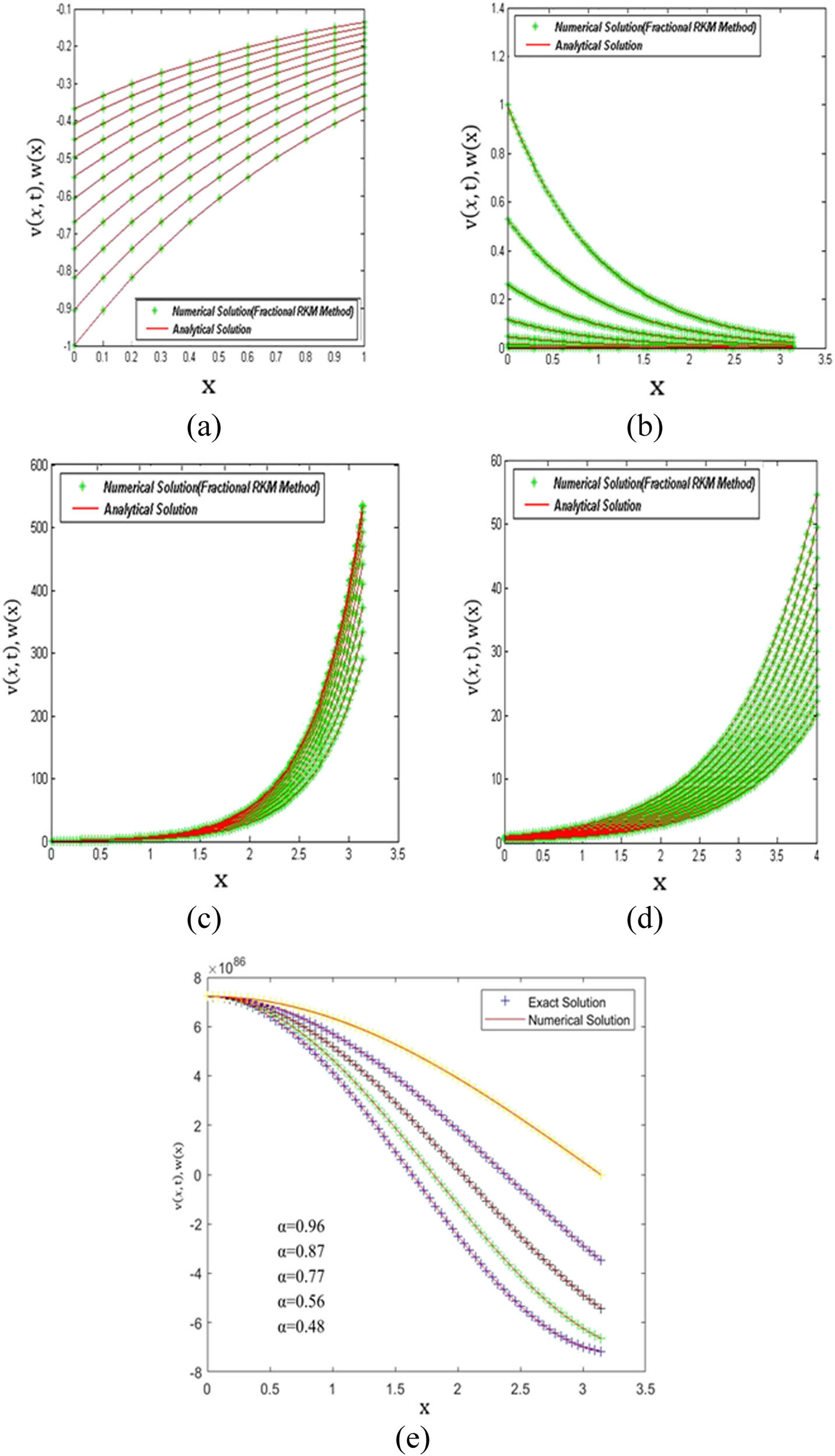
A comparison between the numerical solutions evaluated by generalized numerical methods versus the analytical solutions for the application in Section 4 in (a) and Examples 5.1, 5.2, and 5.3 in (b–d) using generalized RKN and RKM methods, for different values of t, and Example 5.2. with different values of
5 Numerical examples
We implemented the proposed algorithm using the RKM method with N = 6 in Section 3 for solving three different examples of FPDEs using MATLAB software with M = 10, N = 100, and T=1. We tested the proposed methods in this study by the comparisons for the numerical solutions versus exact solutions for three examples in which the numerical solutions on the section line
Example 5.1
Consider the following FPDE problem:
with the I.C.s:
The exact solution is
Example 5.2
Consider the following FPDE problem:
with I.C.s:
The exact solution is
Example 5.3
Consider the following FPDE problem:
with the I.C.s:
with the B.C.s:
The exact solution is
A comparison between the numerical solutions
6 Discussion and conclusion
The main goal of this study is to modify a numerical method for solving FPDEs of different orders. The proposed modified method is used to solve the sixth-order FPDEs in addition to the fractional wave equation, which has been introduced. The implementations are examined for the proposed method. Also, the numerical results are compared with the analytical solutions. From this comparison, we conclude that the proposed approach is an accurate and efficient method. In contrast, the proposed method can be applied to solve PDEs up to the
Acknowledgments
The authors would like to thank the anonymous referees for very helpful comments that have led to an improvement of the article.
-
Funding information: The authors state no funding involved.
-
Author contributions: All authors have accepted responsibility for the entire content of this manuscript and approved its submission.
-
Conflict of interest: The authors state no conflict of interest.
References
[1] Faires JD, Burden R. Numerical Methods. Pacific Grove (CA), USA: Thomson Learning, Inc; 2003.Search in Google Scholar
[2] Farlow SJ. Partial differential equations for scientists and engineers. North Chelmsford (MA), USA: Courier Corporation; 2012.Search in Google Scholar
[3] Salam MA, Obayedullah M, Miah MM. Application of improved kudryashov method to solve nonlinear partial differential equations. J Comput Math Sci. 2016 Apr;7(4):175–80.Search in Google Scholar
[4] Stephenson G. Partial differential equations for scientists and engineers. Singapore: World Scientific; 1996 Jul.10.1142/p018Search in Google Scholar
[5] Damor RS, Kumar S, Shukla AK. Numerical solution of fractional diffusion equation model for freezing in finite media. Int J Eng Math. 2013;2013:1–8. 10.1155/2013/785609.Search in Google Scholar
[6] Zhou MX, Kanth AR, Aruna K, Raghavendar K, Rezazadeh H, Inc M, et al. Numerical solutions of time fractional Zakharov-Kuznetsov equation via natural transform decomposition method with nonsingular kernel derivatives. J Funct Spaces. 2021 Jul;2021:1–7.10.1155/2021/9884027Search in Google Scholar
[7] Momani S, Odibat Z. Comparison between the homotopy perturbation method and the variational iteration method for linear fractional partial differential equations. Comput Math Appl. 2007 Oct;54(7–8):910–9.10.1016/j.camwa.2006.12.037Search in Google Scholar
[8] Jafari H, Jassim HK. Local fractional Laplace variational iteration method for solving nonlinear partial differential equations on Cantor sets within local fractional operators. J Zankoy Sulaimani-Part A. 2014;16(4):49–57.10.17656/jzs.10345Search in Google Scholar
[9] Khan A, Khan A, Khan T, Zaman G. Extension of triple Laplace transform for solving fractional differential equations. Discret Contin Dyn Syst Ser S. 2020 Feb;13(3):755–68.10.3934/dcdss.2020042Search in Google Scholar
[10] Mechee M, Ismail F, Hussain ZM, Siri Z. Direct numerical methods for solving a class of third-order partial differential equations. Appl Math Comput. 2014 Nov;247:663–74.10.1016/j.amc.2014.09.021Search in Google Scholar
[11] Khalaf SL, Flayyih HS. Analysis, predicting, and controlling the COVID-19 pandemic in Iraq through SIR model. Results Control Optim. 2023 Mar;10:100214.10.1016/j.rico.2023.100214Search in Google Scholar
[12] Farhood AK, Mohammed OH. Homotopy perturbation method for solving time-fractional nonlinear Variable-Order Delay Partial Differential Equations. Partial Differ Equ Appl Math. 2023 Jun;7:100513.10.1016/j.padiff.2023.100513Search in Google Scholar
[13] Ford NJ, Xiao J, Yan Y. A finite element method for time fractional partial differential equations. Fract Calc Appl Anal. 2011;14:454–74. 10.2478/s13540-011-0028-2.Search in Google Scholar
[14] Momani S, Odibat Z. Analytical approach to linear fractional partial differential equations arising in fluid mechanics. Phys Lett A. 2006 Jul;355(4–5):271–9.10.1016/j.physleta.2006.02.048Search in Google Scholar
[15] Vanani SK, Aminataei A. Tau approximate solution of fractional partial differential equations. Comput Math Appl. 2011 Aug;62(3):1075–83.10.1016/j.camwa.2011.03.013Search in Google Scholar
[16] Mechee MS, Kadhim MA. Direct explicit integrators of rk type for solving special fourth-order ordinary differential equations with an application. Glob J Pure Appl Math. 2016;12(6):4687–715.10.3844/ajassp.2016.1452.1460Search in Google Scholar
[17] Mechee M, Senu N, Ismail F, Nikouravan B, Siri Z. A three-stage fifth-order Runge-Kutta method for directly solving special third-order differential equation with application to thin film flow problem. Math Probl Eng. 2013 Jan;2013:795397.10.1155/2013/795397Search in Google Scholar
[18] Senu N, Mechee M, Ismail F, Siri Z. Embedded explicit Runge–Kutta type methods for directly solving special third order differential equations y‴ = f (x, y). Appl Math Comput. 2014 Aug;240:281–93.10.1016/j.amc.2014.04.094Search in Google Scholar
[19] Mechee MS. Generalized RK integrators for solving class of sixth-order ordinary differential equations. J Interdiscip Math. 2019 Nov;22(8):1457–61.10.1080/09720502.2019.1705502Search in Google Scholar
[20] Mechee MS, Mshachal JK. Derivation of embedded explicit RK type methods for directly solving class of seventh-order ordinary differential equations. J Interdiscip Math. 2019 Nov;22(8):1451–6.10.1080/09720502.2019.1700936Search in Google Scholar
[21] Singh D, Tiwari BN, Yadav N. Fractional order heat equation in higher space-time dimensions. arXiv preprint arXiv:1704.04101; 2017 Apr.Search in Google Scholar
© 2025 the author(s), published by De Gruyter
This work is licensed under the Creative Commons Attribution 4.0 International License.
Articles in the same Issue
- Research Articles
- Generalized (ψ,φ)-contraction to investigate Volterra integral inclusions and fractal fractional PDEs in super-metric space with numerical experiments
- Solitons in ultrasound imaging: Exploring applications and enhancements via the Westervelt equation
- Stochastic improved Simpson for solving nonlinear fractional-order systems using product integration rules
- Exploring dynamical features like bifurcation assessment, sensitivity visualization, and solitary wave solutions of the integrable Akbota equation
- Research on surface defect detection method and optimization of paper-plastic composite bag based on improved combined segmentation algorithm
- Impact the sulphur content in Iraqi crude oil on the mechanical properties and corrosion behaviour of carbon steel in various types of API 5L pipelines and ASTM 106 grade B
- Unravelling quiescent optical solitons: An exploration of the complex Ginzburg–Landau equation with nonlinear chromatic dispersion and self-phase modulation
- Perturbation-iteration approach for fractional-order logistic differential equations
- Variational formulations for the Euler and Navier–Stokes systems in fluid mechanics and related models
- Rotor response to unbalanced load and system performance considering variable bearing profile
- DeepFowl: Disease prediction from chicken excreta images using deep learning
- Channel flow of Ellis fluid due to cilia motion
- A case study of fractional-order varicella virus model to nonlinear dynamics strategy for control and prevalence
- Multi-point estimation weldment recognition and estimation of pose with data-driven robotics design
- Analysis of Hall current and nonuniform heating effects on magneto-convection between vertically aligned plates under the influence of electric and magnetic fields
- A comparative study on residual power series method and differential transform method through the time-fractional telegraph equation
- Insights from the nonlinear Schrödinger–Hirota equation with chromatic dispersion: Dynamics in fiber–optic communication
- Mathematical analysis of Jeffrey ferrofluid on stretching surface with the Darcy–Forchheimer model
- Exploring the interaction between lump, stripe and double-stripe, and periodic wave solutions of the Konopelchenko–Dubrovsky–Kaup–Kupershmidt system
- Computational investigation of tuberculosis and HIV/AIDS co-infection in fuzzy environment
- Signature verification by geometry and image processing
- Theoretical and numerical approach for quantifying sensitivity to system parameters of nonlinear systems
- Chaotic behaviors, stability, and solitary wave propagations of M-fractional LWE equation in magneto-electro-elastic circular rod
- Dynamic analysis and optimization of syphilis spread: Simulations, integrating treatment and public health interventions
- Visco-thermoelastic rectangular plate under uniform loading: A study of deflection
- Threshold dynamics and optimal control of an epidemiological smoking model
- Numerical computational model for an unsteady hybrid nanofluid flow in a porous medium past an MHD rotating sheet
- Regression prediction model of fabric brightness based on light and shadow reconstruction of layered images
- Dynamics and prevention of gemini virus infection in red chili crops studied with generalized fractional operator: Analysis and modeling
- Qualitative analysis on existence and stability of nonlinear fractional dynamic equations on time scales
- Fractional-order super-twisting sliding mode active disturbance rejection control for electro-hydraulic position servo systems
- Analytical exploration and parametric insights into optical solitons in magneto-optic waveguides: Advances in nonlinear dynamics for applied sciences
- Bifurcation dynamics and optical soliton structures in the nonlinear Schrödinger–Bopp–Podolsky system
- User profiling in university libraries by combining multi-perspective clustering algorithm and reader behavior analysis
- Exploring bifurcation and chaos control in a discrete-time Lotka–Volterra model framework for COVID-19 modeling
- Review Article
- Haar wavelet collocation method for existence and numerical solutions of fourth-order integro-differential equations with bounded coefficients
- Special Issue: Nonlinear Analysis and Design of Communication Networks for IoT Applications - Part II
- Silicon-based all-optical wavelength converter for on-chip optical interconnection
- Research on a path-tracking control system of unmanned rollers based on an optimization algorithm and real-time feedback
- Analysis of the sports action recognition model based on the LSTM recurrent neural network
- Industrial robot trajectory error compensation based on enhanced transfer convolutional neural networks
- Research on IoT network performance prediction model of power grid warehouse based on nonlinear GA-BP neural network
- Interactive recommendation of social network communication between cities based on GNN and user preferences
- Application of improved P-BEM in time varying channel prediction in 5G high-speed mobile communication system
- Construction of a BIM smart building collaborative design model combining the Internet of Things
- Optimizing malicious website prediction: An advanced XGBoost-based machine learning model
- Economic operation analysis of the power grid combining communication network and distributed optimization algorithm
- Sports video temporal action detection technology based on an improved MSST algorithm
- Internet of things data security and privacy protection based on improved federated learning
- Enterprise power emission reduction technology based on the LSTM–SVM model
- Construction of multi-style face models based on artistic image generation algorithms
- Research and application of interactive digital twin monitoring system for photovoltaic power station based on global perception
- Special Issue: Decision and Control in Nonlinear Systems - Part II
- Animation video frame prediction based on ConvGRU fine-grained synthesis flow
- Application of GGNN inference propagation model for martial art intensity evaluation
- Benefit evaluation of building energy-saving renovation projects based on BWM weighting method
- Deep neural network application in real-time economic dispatch and frequency control of microgrids
- Real-time force/position control of soft growing robots: A data-driven model predictive approach
- Mechanical product design and manufacturing system based on CNN and server optimization algorithm
- Application of finite element analysis in the formal analysis of ancient architectural plaque section
- Research on territorial spatial planning based on data mining and geographic information visualization
- Fault diagnosis of agricultural sprinkler irrigation machinery equipment based on machine vision
- Closure technology of large span steel truss arch bridge with temporarily fixed edge supports
- Intelligent accounting question-answering robot based on a large language model and knowledge graph
- Analysis of manufacturing and retailer blockchain decision based on resource recyclability
- Flexible manufacturing workshop mechanical processing and product scheduling algorithm based on MES
- Exploration of indoor environment perception and design model based on virtual reality technology
- Tennis automatic ball-picking robot based on image object detection and positioning technology
- A new CNN deep learning model for computer-intelligent color matching
- Design of AR-based general computer technology experiment demonstration platform
- Indoor environment monitoring method based on the fusion of audio recognition and video patrol features
- Health condition prediction method of the computer numerical control machine tool parts by ensembling digital twins and improved LSTM networks
- Establishment of a green degree evaluation model for wall materials based on lifecycle
- Quantitative evaluation of college music teaching pronunciation based on nonlinear feature extraction
- Multi-index nonlinear robust virtual synchronous generator control method for microgrid inverters
- Manufacturing engineering production line scheduling management technology integrating availability constraints and heuristic rules
- Analysis of digital intelligent financial audit system based on improved BiLSTM neural network
- Attention community discovery model applied to complex network information analysis
- A neural collaborative filtering recommendation algorithm based on attention mechanism and contrastive learning
- Rehabilitation training method for motor dysfunction based on video stream matching
- Research on façade design for cold-region buildings based on artificial neural networks and parametric modeling techniques
- Intelligent implementation of muscle strain identification algorithm in Mi health exercise induced waist muscle strain
- Optimization design of urban rainwater and flood drainage system based on SWMM
- Improved GA for construction progress and cost management in construction projects
- Evaluation and prediction of SVM parameters in engineering cost based on random forest hybrid optimization
- Museum intelligent warning system based on wireless data module
- Optimization design and research of mechatronics based on torque motor control algorithm
- Special Issue: Nonlinear Engineering’s significance in Materials Science
- Experimental research on the degradation of chemical industrial wastewater by combined hydrodynamic cavitation based on nonlinear dynamic model
- Study on low-cycle fatigue life of nickel-based superalloy GH4586 at various temperatures
- Some results of solutions to neutral stochastic functional operator-differential equations
- Ultrasonic cavitation did not occur in high-pressure CO2 liquid
- Research on the performance of a novel type of cemented filler material for coal mine opening and filling
- Testing of recycled fine aggregate concrete’s mechanical properties using recycled fine aggregate concrete and research on technology for highway construction
- A modified fuzzy TOPSIS approach for the condition assessment of existing bridges
- Nonlinear structural and vibration analysis of straddle monorail pantograph under random excitations
- Achieving high efficiency and stability in blue OLEDs: Role of wide-gap hosts and emitter interactions
- Construction of teaching quality evaluation model of online dance teaching course based on improved PSO-BPNN
- Enhanced electrical conductivity and electromagnetic shielding properties of multi-component polymer/graphite nanocomposites prepared by solid-state shear milling
- Optimization of thermal characteristics of buried composite phase-change energy storage walls based on nonlinear engineering methods
- A higher-performance big data-based movie recommendation system
- Nonlinear impact of minimum wage on labor employment in China
- Nonlinear comprehensive evaluation method based on information entropy and discrimination optimization
- Application of numerical calculation methods in stability analysis of pile foundation under complex foundation conditions
- Research on the contribution of shale gas development and utilization in Sichuan Province to carbon peak based on the PSA process
- Characteristics of tight oil reservoirs and their impact on seepage flow from a nonlinear engineering perspective
- Nonlinear deformation decomposition and mode identification of plane structures via orthogonal theory
- Numerical simulation of damage mechanism in rock with cracks impacted by self-excited pulsed jet based on SPH-FEM coupling method: The perspective of nonlinear engineering and materials science
- Cross-scale modeling and collaborative optimization of ethanol-catalyzed coupling to produce C4 olefins: Nonlinear modeling and collaborative optimization strategies
- Unequal width T-node stress concentration factor analysis of stiffened rectangular steel pipe concrete
- Special Issue: Advances in Nonlinear Dynamics and Control
- Development of a cognitive blood glucose–insulin control strategy design for a nonlinear diabetic patient model
- Big data-based optimized model of building design in the context of rural revitalization
- Multi-UAV assisted air-to-ground data collection for ground sensors with unknown positions
- Design of urban and rural elderly care public areas integrating person-environment fit theory
- Application of lossless signal transmission technology in piano timbre recognition
- Application of improved GA in optimizing rural tourism routes
- Architectural animation generation system based on AL-GAN algorithm
- Advanced sentiment analysis in online shopping: Implementing LSTM models analyzing E-commerce user sentiments
- Intelligent recommendation algorithm for piano tracks based on the CNN model
- Visualization of large-scale user association feature data based on a nonlinear dimensionality reduction method
- Low-carbon economic optimization of microgrid clusters based on an energy interaction operation strategy
- Optimization effect of video data extraction and search based on Faster-RCNN hybrid model on intelligent information systems
- Construction of image segmentation system combining TC and swarm intelligence algorithm
- Particle swarm optimization and fuzzy C-means clustering algorithm for the adhesive layer defect detection
- Optimization of student learning status by instructional intervention decision-making techniques incorporating reinforcement learning
- Fuzzy model-based stabilization control and state estimation of nonlinear systems
- Optimization of distribution network scheduling based on BA and photovoltaic uncertainty
- Tai Chi movement segmentation and recognition on the grounds of multi-sensor data fusion and the DBSCAN algorithm
- Special Issue: Dynamic Engineering and Control Methods for the Nonlinear Systems - Part III
- Generalized numerical RKM method for solving sixth-order fractional partial differential equations