Haar wavelet collocation method for existence and numerical solutions of fourth-order integro-differential equations with bounded coefficients
-
Rohul Amin
 ,
Muhammad Nawaz
,
Muhammad Nawaz

Abstract
In this article, Haar wavelet collocation method is applied for the solution of fourth-order integro-differential equations. Also, a fixed point approach is used to investigate the existence theory of solution to the considered problem. The fourth-order derivative is approximated using Haar function. In addition, third-, second-, and first-order derivatives together with unknown functions are obtained by the process of successive integrations. On applying the Haar collocation method, the suggested problem of IDEs is transformed to a system of algebraic equations. The Gauss elimination scheme is used for the solution of linear algebraic equations. The precision, effectiveness, and convergence of the Haar approach are checked on some test problems. Different collocation and Gauss points are used to determine the absolute and root mean square errors. To demonstrate the applicability of the proposed method, an experimental rate of convergence is calculated, which is almost equal to 2. The method is accurate, easily applicable, and efficient.
1 Introduction
Functional equations, such as partial differential equations (PDEs), integral and integro-differential equations (IDEs), stochastic equations, and others, are typically the outcome of mathematical modelling of real-world issues. IDEs are found in many mathematical formulations of physical processes and are used in chemical kinetics, fluid dynamics, and biological models (for more information, see [1]). IDEs are frequently encountered in problems involving electrostatics, low-frequency electromagnetism, electromagnetism scattering, and the propagation of elastic and acoustic waves. Some applications in scientific disciplines, including microscopy, seismology, radio astronomy, electron emission, atomic scattering, radar range, plasma diagnostics, X-ray radiography, and optical fibre evaluation, when formulated, we obtain in the form of IDEs [2]. Numerous topics are covered in the said area, for instance, the Volterra population growth model, coexisting biological species, the spread of stocked fish in a new lake, heat radiation, and heat transfer. Usually, it is difficult to obtain the exact or analytical solution for every IDEs; therefore, researchers have always tried to establish sophisticated numerical tools to study such problems for their approximate solutions.
Many researchers worked to compute the approximate solution of fourth-order IDEs. Sweilam [3] has used a variational iteration technique (VIT) for the solution of IDEs of order four. Linear and nonlinear fourth-order IDEs have been solved using VIT with boundary conditions. Sweilam et al. [4] have developed a scheme for the solution of fourth-order IDEs based on the pseudo-spectral procedure. Lakestani and Deghan [5] used Chebyshev functions for approximate solutions of fourth-order IDEs. This technique involves expanding the desired solution as Chebyshev cardinal functions. They convert the IDEs to a system of algebraic equations by using an operational matrix. Ghomanjani et al. [6] used the Bezier curve technique to find an approximate solution of fourth-order IDEs. Based on the Adomian decomposition technique, Singh and Wazwaz [7] developed a numerical scheme to address fourth-order boundary value problems (BVPs) of Volterra IDEs. For a recursive method of solution, they applied the Green functions to transform IDEs into integral equations.
The Haar wavelet collocation (HWC) technique is used for different problems in the literature. Some applications of the HWC technique for Lane–Emden equations [8], nonlinear delay IDEs [9], nonlinear delay integral equations [10], software piracy [11], fractional delay differential equations (DEs) [12,13], fractional IDEs [14,15], third-order boundary-value problems of IDEs [16], system of fractional DEs [17], Burger’s equations [18], Schrodinger’s equations [19], inverse problems [20], and interface problems [21]. Majak et al. [22] introduced a higher order Haar wavelet method. Additionally, this technique is used for DEs [23], vibration analysis of beams [24,25], integral equations [26], IDEs [17], nonlinear PDEs [27], and nonlinear evolution equations [28].
Wu et al. [29] used a homotopy-based stochastic finite-element model updating method to cope with the correlation of static measurement data. Cai et al. [30] studies dynamically controlling terahertz wavefronts with cascaded metasurfaces. Yang and Kai [31] studied the nonlinear coupled Schrödinger equation in fibre Bragg gratings. Zhou et al. [32] developed an iterative threshold algorithm for the sparse optimization problems with a log-sum function. Jiang et al. [33] modeled the uncertainty mechanism using an inclusiveness function for each agent to capture the acceptance degree of opposing opinions. The main advantages of this method are its simplicity and less computation costs: it is due to the sparsity of the transform matrices and the small number of significant wavelet coefficients. The Haar method stands out due to its computational efficiency, direct approximation of solutions, ability to handle discontinuities, and flexibility, especially in solving nonlinear IDEs. Its advantages over traditional methods like Laplace, Sumudu, and others make it a powerful tool in numerical analysis, particularly when solving problems require high accuracy with fewer computational resources [34].
Existence theory is an important consequence of applied analysis. The said analysis is used to investigate whether a particular problem that is under investigation has a solution or not. For this purpose, an important theory was founded by Banach in 1922. After him, many theories and results were established to study the existence theory of solutions for integral, functional, algebraic, and DEs. Previous studies [35–37] have valuable contributions to the theory of existence of solutions. This theory tells us whether the problem has a solution or not. If yes, how many solutions are there for a particular problem? Therefore, fixed point theory and nonlinear analysis tools like the degree theories of Mawhin and Schauder have gained much attention in the last few decades. We refer to some work like [38–40]. Here, we remark that the existence theory of IDEs has also been considered recently by many researchers in their work. For instance, Shatanawii et al. [41] have studied the existence of solutions to some integral problems. In the same way, Shatanawii et al. [42] and Isik et al. [43] established the existence theory for some IDE problems.
In this study, fourth-order linear Volterra–Fredholm IDEs are solved using the HWC technique. Consider the subsequent fourth-order linear IDE:
subject to
where
subject to
here
The structure of this article is as follows. Section 2 addresses Haar functions, and Section 3 presents existence and uniqueness results. The numerical scheme for solving nonlinear fourth-order IDEs is provided in Section 4. In Section 5, convergence is provided. Examples from the literature are provided in Section 6. Section 7 presents the results and comments. Section 8 provides the conclusion.
2 Haar wavelet
The scaling function is [9]
The Mother wavelet is given by
The dilation and translation operations provide
where
For purposes of approximation, this is truncated at
we use the symbol
and the definition of
Through integral simplification, we can obtain the values of
The value of
If
The interval
The points
3 Existence and uniqueness results
This section is related to existing results. Let denotes
We make some assumptions that will be used in the main result:
Since
Since
Further, we write (13) as
Theorem 3.1
Under hypotheses
then (1) has a unique solution.
Proof
Let
Since
which gives
Now, from Eq. (20), we have for any
hence, we have
also from Eq. (21), we have
also from Eq. (22), we have
Now,
and
Thus, Eq. (27) implies that
In view of this result, we can claim that Eq. (1) has a unique solution.□
The solution of nonlinear problem Eq. (2) can be written in equivalent integral form as
Note: Since we see that
Theorem 3.2
In view of assumptions (
holds.
Proof
The proof is similar and can be followed by the same process as done in Theorem 3.1.□
4 Numerical method
Here, HWC technique is developed for the solution of fourth-order Volterra–Fredholm IDEs. The integration method yields expression for lower derivatives, whereas the Haar function approximates the fourth-order derivative. Additionally, formula (30) is used to obtain the integral involved in Eq. (1)
We can obtain the algebraic equations system by placing the CPs and GPs in Eq. (1) and using the HWC technique to it. The unknown Haar coefficients are found using the Gauss elimination method. Ultimately, solution at the CPs is obtained by use of these coefficients. Consider
Integrating from 0 to
Using the initial condition, we have
Again integrating from 0 to
After establishing an initial condition, we have
Again integrating from 0 to
Again using the initial condition, we have
Integrating from 0 to
Using the initial conditions and rearranging, we have
Eq. (34) is known as numerical solution.
4.1 Solution of Volterra–Fredholm fourth-order IDEs
4.1.1 Linear case
Numerical integration of Eq. (1) yields the following equation:
By putting values in Eq. (37), we have
After rearranging, we obtain
By putting CPs
The
4.1.2 Nonlinear case
Numerical integration of Eq. (2) yields the following equation:
By putting values in Eq. (2), we have
After rearranging, we obtain
By putting CPs
This is an
5 Convergence
Theorem 5.1
Let
where
This section uses the HWC technique on certain cases to demonstrate the accuracy as well as efficacy of the suggested methods. The absolute error is represented by
At CPs and GPs, root mean square error is described as
Rate of convergence at CPs and GPs is denoted by
6 Numerical examples
Here, we enrich our article by providing some examples to elaborate the numerical scheme.
Example 6.1
Consider the fourth-order IDE:
with ICs
The exact solution is
Example 6.2
Consider the fourth-order linear FIDE:
with ICs
The exact solution is
Example 6.3
Consider the linear Fredholm-Volterra IDE
ICs are
Example 6.4
Consider the fourth-order BVP IDE [7]:
with boundary conditions
The exact solution is
Example 6.5
Consider the nonlinear Fredholm IDE
with initial condition
Example 6.6
Consider the nonlinear Volterra IDE
with initial condition
Example 6.7
Consider the following nonlinear Volterra–Fredholm fourth-order IDE as
The exact solution is given by
7 Results and discussion
The numerical results for linear Volterra, Fredholm, and Volterra–Fredholm fourth-order IDEs are reported in Tables 1, 2, 3, 4, , 6 and 7. The results of our proposed method are compared with [7], which is shown in Table 5.
|
|
|
|
|
|
|
|
|---|---|---|---|---|---|---|
| 2 |
|
— |
|
— |
|
|
|
|
|
1.6931 |
|
1.7213 |
|
|
|
|
|
1.8568 |
|
1.8743 |
|
|
|
|
|
1.9307 |
|
1.9400 |
|
|
|
|
|
1.9659 |
|
1.9706 |
|
|
|
|
|
1.9831 |
|
1.9854 |
|
|
|
|
|
1.9916 |
|
1.9928 |
|
|
|
|
|
1.9971 |
|
1.9983 |
|
|
|
|
|
|
|
|
|
|
|---|---|---|---|---|---|---|
| 2 |
|
— |
|
— |
|
|
|
|
|
1.6808 |
|
1.7301 |
|
|
|
|
|
1.8469 |
|
1.8743 |
|
|
|
|
|
1.9249 |
|
1.9389 |
|
|
|
|
|
1.9628 |
|
1.9699 |
|
|
|
|
|
1.9815 |
|
1.9850 |
|
|
|
|
|
1.9908 |
|
1.9925 |
|
|
|
|
|
1.9975 |
|
1.9978 |
|
|
|
|
|
|
|
|
|
|
|---|---|---|---|---|---|---|
|
|
|
— |
|
— |
|
|
|
|
|
1.9361 |
|
1.9666 |
|
|
|
|
|
1.9734 |
|
1.9877 |
|
|
|
|
|
1.9880 |
|
1.9949 |
|
|
|
|
|
1.9944 |
|
1.9977 |
|
|
|
|
|
1.9972 |
|
1.9989 |
|
|
|
|
|
1.9986 |
|
1.9994 |
|
|
|
|
|
1.9993 |
|
1.9997 |
|
|
|
|
|
1.9996 |
|
1.9998 |
|
|
|
|
|
|
|
|
|
|
|---|---|---|---|---|---|---|
| 2 |
|
— |
|
— |
|
|
|
|
|
1.6858 |
|
1.7298 |
|
|
|
|
|
1.8493 |
|
1.8754 |
|
|
|
|
|
1.9260 |
|
1.9397 |
|
|
|
|
|
1.9633 |
|
1.9703 |
|
|
|
|
|
1.9818 |
|
1.9852 |
|
|
|
|
|
1.9909 |
|
1.9927 |
|
|
|
|
|
1.9955 |
|
1.9963 |
|
|
|
|
|
|
|
|
|
|
|---|---|---|---|---|---|---|
| 2 |
|
— |
|
— |
|
|
|
|
|
1.6910 |
|
1.7295 |
|
|
|
|
|
1.7529 |
|
1.8755 |
|
|
|
|
|
1.7964 |
|
1.7907 |
|
|
|
|
|
1.8245 |
|
2.1194 |
|
|
|
|
|
1.8424 |
|
1.9185 |
|
|
|
|
|
1.8754 |
|
1.9853 |
|
|
|
|
|
HWC
|
|---|---|---|
| 0.1 |
|
|
| 0.3 |
|
|
| 0.5 |
|
|
| 0.7 |
|
|
| 0.9 |
|
|
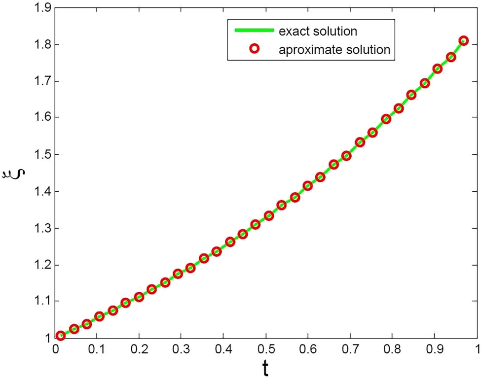
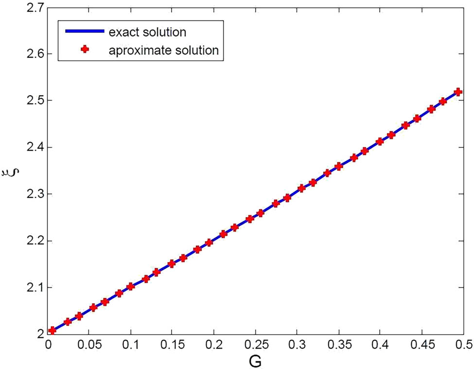
Comparisons of numerical and the exact solutions for 32 CPs of Example 6.1.
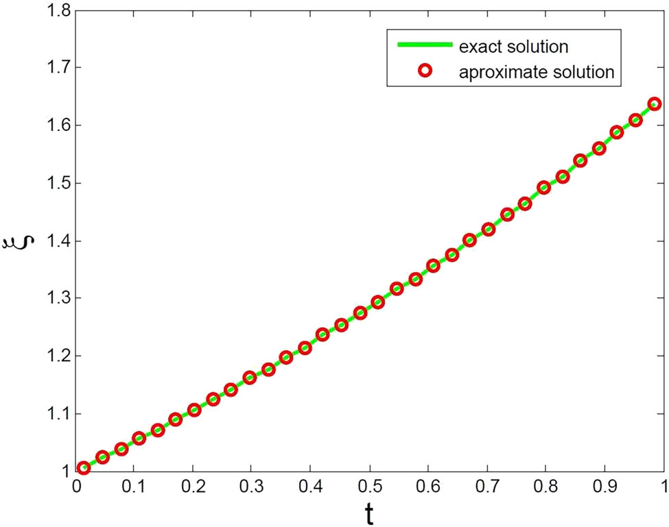
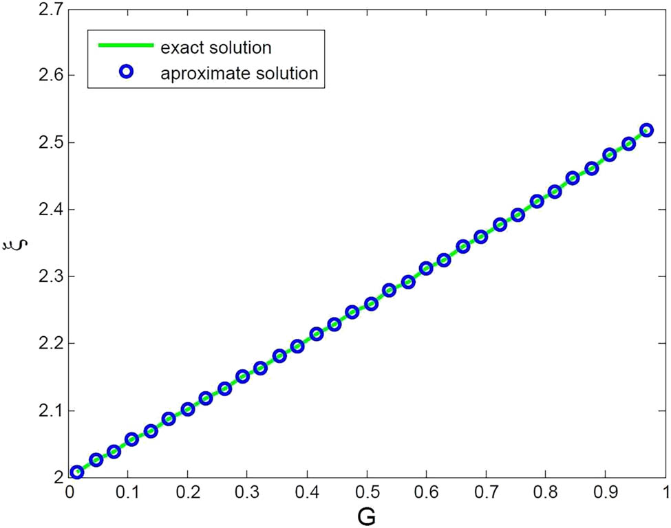
Comparisons of numerical and the exact solutions for 32 CPs of Example 6.2.
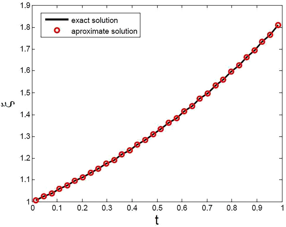
Comparison of numerical and exact solutions for 32 CPs of Example 6.3.
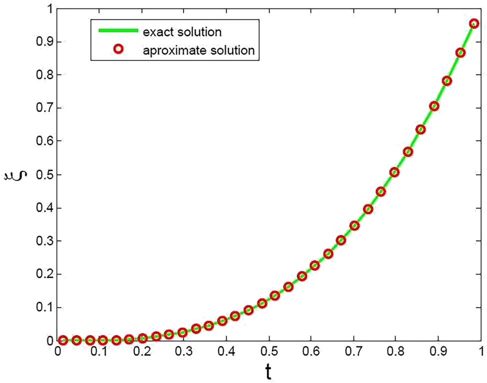
Comparison of numerical and exact solutions for 32 CPs of Example 6.7.
Comparison of numerical and exact solutions for 32 CPs of Example 6.5.
Comparison of numerical and exact solutions for 32 CPs of Example 6.6.
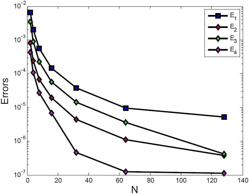
Comparison of different errors for Example 6.7.
|
|
|
|
|
|
|
|
|---|---|---|---|---|---|---|
| 2 |
|
— |
|
— |
|
|
|
|
|
1.5011 |
|
1.4255 |
|
|
|
|
|
1.5921 |
|
1.5528 |
|
|
|
|
|
1.6423 |
|
1.7123 |
|
|
|
|
|
1.6931 |
|
1.8084 |
|
|
|
|
|
1.7940 |
|
1.9001 |
|
|
|
|
|
1.8623 |
|
1.9397 |
|
|
|
|
|
|
|
|
|
|
|---|---|---|---|---|---|---|
| 2 |
|
— |
|
— |
|
|
|
|
|
1.5012 |
|
1.6201 |
|
|
|
|
|
1.6102 |
|
1.7778 |
|
|
|
|
|
1.6301 |
|
1.8406 |
|
|
|
|
|
1.7290 |
|
1.9407 |
|
|
|
|
|
1.8244 |
|
1.9991 |
|
|
|
|
|
1.9901 |
|
2.0215 |
|
|
8 Conclusion
In this study, the solution to fourth-order IDEs has been studied by using the HWC technique. We have established few prerequisites for the presented problem’s like existence and uniqueness of solution by the application of fixed point analysis. We have established an algorithm for the computation via using HWC tools. Then, several examples were investigated to demonstrate our results. For the validation of our procedure, maximum absolute errors for various CPs have been recorded in several tables. A comparison of the exact solution has been made with the numerical solution for the considered examples. Figures have been used to compare the exact and approximate solutions for each example. The suggested scheme showed better accuracy and effectiveness which can be further improved by increasing the number of CPs. The MATLAB 2016 software has been used for all computational tasks. In future, we plan to extend the HWC technique for solution of higher order IDEs, fractional order IDEs, system of IDEs, IDEs with two point and integral boundary conditions, and 2D and 3D problems of higher order IDEs or statements.
Acknowledgment
K. Sha and T. Abdeljawad are thankful to Prince Sultan University for APC and support through the TAS research lab.
-
Funding information: The authors state no funding involved.
-
Author contributions: All authors have approved the final version of the manuscript. R. A., M. N., K. S., and T. A. wrote the main manuscript, and R. A. and M. N. prepared the tables figures and reviewed the manuscript.
-
Conflict of interest: The authors state no conflict of interest.
-
Data availability statement: The data used in this research are included within the article.
References
[1] Kythe PK, Puri P. Computational methods for linear integral equations. New Orleans: University of New Orleans; 2002. 10.1007/978-1-4612-0101-4Search in Google Scholar
[2] Wazwaz AM. Linear and nonlinear integral equations. Berlin: Springer; 2011. 10.1007/978-3-642-21449-3Search in Google Scholar
[3] Sweilam NH. Fourth order integro-differential equations using variational iteration method. Comput Math Appl. 2007;54:1086–91. 10.1016/j.camwa.2006.12.055Search in Google Scholar
[4] Sweilam NH, Khader MM, Kota WY. Numerical and analytical study for fourth-order integro-differential equations using a pseudospectral method. Meth Probs Eng. 2013;2013:1–8. 10.1155/2013/434753Search in Google Scholar
[5] Lakestani M, Deghan M. Numerical solution of fourth-order integro-differential equations using Chebyshev cardinal functions. Int J Comput Math. 2010;87:1389–94. 10.1080/00207160802322357Search in Google Scholar
[6] Ghomanjani F, Kamyad AV, Kilicman A. Bezier curves method for fourth-order integro-differential equations. Abstr Appl Anal. 2013;2013:1–5. 10.1155/2013/672058Search in Google Scholar
[7] Singh R, Wazwaz AM. Numerical solutions of fourth-order Volterra integro-differential equations by the Green function and decomposition method. Meth Sci. 2016;10:159–66. 10.1007/s40096-016-0190-0Search in Google Scholar
[8] Singh R, Garg H, Guleria V. Haar wavelet collocation method for Lane-Emden equations with Dirichlet, Neumann, and Neumann-Robin boundary conditions. J Comput Appl Math. 2019;346:150–61. 10.1016/j.cam.2018.07.004Search in Google Scholar
[9] Islam S, Aziz I, Al-Fhaid AS. An improved method based on Haar wavelets for numerical solution of nonlinear integral and integro-differential equations of first and higher orders. J Comput Appl Math. 2014;260:449–69. 10.1016/j.cam.2013.10.024Search in Google Scholar
[10] Erfanian M, Mansoori A. Solving the nonlinear integro-differential equation in complex plane with rationalized Haar wavelet. Math Comput Simul. 2019;165:223–37. 10.1016/j.matcom.2019.03.006Search in Google Scholar
[11] Nazir S, Shahzad S, Wirza R, Amin R, Ahsan M, Mukhtar N, et al. Birthmark based identification of software piracy using Haar wavelet. Math Comput Simul. 2019;166:144–54. 10.1016/j.matcom.2019.04.010Search in Google Scholar
[12] Erfanian M, Zeidabadi H. Solving nonlinear Fredholm integro-differential equations in a complex plane with rationalized Haar wavelet bases. Asian-European J Math. 2019;12(4):1950055. 10.1142/S1793557119500554Search in Google Scholar
[13] Mohammad NA, Sabawi YA, Hasso MS. Haar wavelet method for the numerical solution of nonlinear Fredholm integro-differential equations. J Educ Sci. 2023;32(4):10–25. 10.33899/edusj.2023.139892.1360Search in Google Scholar
[14] Amin R, Shah K, Asif M, Khan I, Ullah F. An efficient algorithm for numerical solution of fractional integro-differential equations via Haar wavelet. J Comput Appl Math. 2021;381:113028. 10.1016/j.cam.2020.113028Search in Google Scholar
[15] Amin R, Ahmad H, Shah K, Hafeez MB, Sumelka W. Theoretical and computational analysis of nonlinear fractional integro-differential equations via collocation method. Chaos Solitons Fractals. 2021;151:111252. 10.1016/j.chaos.2021.111252Search in Google Scholar
[16] Alqarni MM, Amin R, Shah K, Nazir S, Awais M, Mahmoud E. Solution of third-order linear and nonlinear boundary value problems of integro-differential equations using Haar wavelet method. Results Phys. 2021;25:104176. 10.1016/j.rinp.2021.104176Search in Google Scholar
[17] Ahsan M, Lei W, Alwuthaynani M, Ahmad M, Nisar M. A higher-order collocation method based on Haar wavelets for integro-differential equations with two-point integral condition. Phys Scr. 2023;99:015211. 10.1088/1402-4896/ad1089Search in Google Scholar
[18] Zada L, Aziz I. The numerical solution of fractional Korteweg-de Vries and Burgers’ equations via Haar wavelet. Math Meth Appl Sci. 2021;44:10564–77. 10.1002/mma.7430Search in Google Scholar
[19] Karabas NI, Korkut SO, Tanoglu G, Aziz I. An efficient approach for solving nonlinear multidimensional Schrödinger equations. Eng Anal Bound Elements. 2021;132:263–70. 10.1016/j.enganabound.2021.07.009Search in Google Scholar
[20] Ahsan M, Haq KS, Liu X, Lone SA, Nisar M. A Haar wavelets based approximation for nonlinear inverse problems influenced by unknown heat source. Math Meth Appl Sci. 2023;46:2475–87. 10.1002/mma.8655Search in Google Scholar
[21] Asif M, Bilal F, Bilal R, Haider N, Abdelmohsenc SA, Eldind SM. An efficient algorithm for the numerical solution of telegraph interface model with discontinuous coefficients via Haar wavelets. Alex Eng J. 2023;72:275–85. 10.1016/j.aej.2023.03.074Search in Google Scholar
[22] Majak J, Pohlak M, Karjust K, Eerme M, Kurnitski J, Shvartsman B. New higher order Haar wavelet method: application to FGM structures. Compos Struct. 2018;201:72–8. 10.1016/j.compstruct.2018.06.013Search in Google Scholar
[23] Majak J, Shvartsman B, Pohlak M, Karjust K, Eerme M, Tungel E. Solving ordinary differential equations with higher order Haar wavelet method. AIP Conf Proc. 2019;2116:330002. 10.1063/1.5114340Search in Google Scholar
[24] Majak J, Shvartsman B, Ratas M, Bassir D, Pohlak M, Karjust K, et al. Higher-order Haar wavelet method for vibration analysis of nanobeams. Mater Today Commun. 2020;25:101290. 10.1016/j.mtcomm.2020.101290Search in Google Scholar
[25] Mehrparvar M, Majak J, Karjust K, Arda M. Free vibration analysis of tapered Timoshenko beam with higher order Haar wavelet method. Proc Est Acad Sci. 2022;71:77–83. 10.3176/proc.2022.1.07Search in Google Scholar
[26] Ratas M, Salupere A. Application of higher order Haar wavelet method for solving nonlinear evolution equations. Math Model Anal. 2020;25:271–88. 10.3846/mma.2020.11112Search in Google Scholar
[27] Ratas M, Salupere A, Majak J. Solving nonlinear PDEs using the higher order Haar wavelet method on nonuniform and adaptive grids. Math Model Anal. 2021;26:147–69. 10.3846/mma.2021.12920Search in Google Scholar
[28] Yasmeen S, Islam S, Amin R. Higher order Haar wavelet method for numerical solution of integral equations. Comput Appl Math. 2023;42:147. 10.1007/s40314-023-02283-0Search in Google Scholar
[29] Wuuu Z, Huang B, Fan J, Chen H. Homotopy based stochastic finite element model updating with correlated static measurement data. Measurement. 2023;210:112512. 10.1016/j.measurement.2023.112512Search in Google Scholar
[30] Cai X, Tang R, Zhou H, Li Q, Ma S, Wang D, et al. Dynamically controlling terahertz wavefronts with cascaded metasurfaces. Adv Photon. 2021;3(3):036003. 10.1117/1.AP.3.3.036003Search in Google Scholar
[31] Yang R, Kai Y. Dynamical properties, modulation instability analysis and chaotic behaviors to the nonlinear coupled Schrödinger equation in fiber Bragg gratings. Modern Phys Lett B. 2023;38:2350239. 10.1142/S0217984923502391Search in Google Scholar
[32] Zhou X, Liu X, Zhang G, Jia L, Wang X, Zhao Z. An iterative threshold algorithm of log-sum regularization for sparse problem. IEEE Trans Circuits Syst Video Tech. 2023;33(9):4728–40. 10.1109/TCSVT.2023.3247944Search in Google Scholar
[33] Jiang B, Zhao Y, Dong J, Hu J. Analysis of the influence of trust in opposing opinions: An inclusiveness-degree based Signed Deffuant-Weisbush model. Inform Fusion. 2024;104:102173. 10.1016/j.inffus.2023.102173Search in Google Scholar
[34] Arefi M, Jafari S. Comparison of Haar wavelet method and other integral transforms for Volterra equations. Math Meth Appl Sci. 2015;38:365–74. Search in Google Scholar
[35] Agarwal RP, Meehan M, O’Regan D. Fixed point theory and applications. Cambridge, UK: Cambridge University Press; 2001. 10.1017/CBO9780511543005Search in Google Scholar
[36] Argyros IK, Hilout S. Computational methods in nonlinear analysis: efficient algorithms, fixed point theory and applications. Singapore: World Scientific; 2013. 10.1142/8475Search in Google Scholar
[37] Cho YJ, Kim JK, Kang SM. Fixed point theory and Applications. New York, USA: Nova Publishers; 2007. Search in Google Scholar
[38] Karapinar E. Fixed point theorems in cone Banach spaces. Fixed Point Theory Appl. 2009;2009:1–9. 10.1155/2009/609281Search in Google Scholar
[39] Park C. Fixed points and Hyers-Ulam-Rassias stability of Cauchy-Jensen functional equations in Banach algebras. Fixed Point Theory and Appl. 2007;2007:1–15. 10.1155/2007/50175Search in Google Scholar
[40] Amar AB, Jeribi A, Mnif M. Some fixed point theorems and application to biological models. Num Funct Anal Optim. 2008;29(1–2):1–23. 10.1080/01630560701749482Search in Google Scholar
[41] Shatnawi TA, Boudaoui A, Shatanawi W, Laksaci N. Solvability of a system of integral equations in two variables in the weighted Sobolev space W(1,1)−ω(a,b) using a generalized measure of noncompactness. Nonl Model Control. 2022;27:1–21. 10.15388/namc.2022.27.27961Search in Google Scholar
[42] Shatanawi W, Mlaiki N, Rizk D, Onunwor E. Fredholm-type integral equation in controlled metric-like spaces. Adv Diff Equ. 2021;2021(1):1–13. 10.1186/s13662-021-03516-4Search in Google Scholar
[43] Isik H, Moeini B, Aydi H, Mlaiki N. Fixed points of subadditive maps with an application to a system of Volterra-Fredholm type integro-differential equations. Math Prob Eng. 2019;2019:1–9. 10.1155/2019/6925891Search in Google Scholar
[44] Majak J, Shvartsman BS, Kirs M, Pohlak M, Herranen H. Convergence theorem for the Haar wavelet based discretization method. Comp Struct. 2015;126:227–32. 10.1016/j.compstruct.2015.02.050Search in Google Scholar
[45] Majak J, Shvartsman BS, Karjust K, Mikola M, Haavajoe A, Pohlak M. On the accuracy of the Haar wavelet discretization method. Comp Eng. 2015;80:321–7. 10.1016/j.compositesb.2015.06.008Search in Google Scholar
© 2025 the author(s), published by De Gruyter
This work is licensed under the Creative Commons Attribution 4.0 International License.
Articles in the same Issue
- Research Articles
- Generalized (ψ,φ)-contraction to investigate Volterra integral inclusions and fractal fractional PDEs in super-metric space with numerical experiments
- Solitons in ultrasound imaging: Exploring applications and enhancements via the Westervelt equation
- Stochastic improved Simpson for solving nonlinear fractional-order systems using product integration rules
- Exploring dynamical features like bifurcation assessment, sensitivity visualization, and solitary wave solutions of the integrable Akbota equation
- Research on surface defect detection method and optimization of paper-plastic composite bag based on improved combined segmentation algorithm
- Impact the sulphur content in Iraqi crude oil on the mechanical properties and corrosion behaviour of carbon steel in various types of API 5L pipelines and ASTM 106 grade B
- Unravelling quiescent optical solitons: An exploration of the complex Ginzburg–Landau equation with nonlinear chromatic dispersion and self-phase modulation
- Perturbation-iteration approach for fractional-order logistic differential equations
- Variational formulations for the Euler and Navier–Stokes systems in fluid mechanics and related models
- Rotor response to unbalanced load and system performance considering variable bearing profile
- DeepFowl: Disease prediction from chicken excreta images using deep learning
- Channel flow of Ellis fluid due to cilia motion
- A case study of fractional-order varicella virus model to nonlinear dynamics strategy for control and prevalence
- Multi-point estimation weldment recognition and estimation of pose with data-driven robotics design
- Analysis of Hall current and nonuniform heating effects on magneto-convection between vertically aligned plates under the influence of electric and magnetic fields
- A comparative study on residual power series method and differential transform method through the time-fractional telegraph equation
- Insights from the nonlinear Schrödinger–Hirota equation with chromatic dispersion: Dynamics in fiber–optic communication
- Mathematical analysis of Jeffrey ferrofluid on stretching surface with the Darcy–Forchheimer model
- Exploring the interaction between lump, stripe and double-stripe, and periodic wave solutions of the Konopelchenko–Dubrovsky–Kaup–Kupershmidt system
- Computational investigation of tuberculosis and HIV/AIDS co-infection in fuzzy environment
- Signature verification by geometry and image processing
- Theoretical and numerical approach for quantifying sensitivity to system parameters of nonlinear systems
- Chaotic behaviors, stability, and solitary wave propagations of M-fractional LWE equation in magneto-electro-elastic circular rod
- Dynamic analysis and optimization of syphilis spread: Simulations, integrating treatment and public health interventions
- Visco-thermoelastic rectangular plate under uniform loading: A study of deflection
- Threshold dynamics and optimal control of an epidemiological smoking model
- Numerical computational model for an unsteady hybrid nanofluid flow in a porous medium past an MHD rotating sheet
- Regression prediction model of fabric brightness based on light and shadow reconstruction of layered images
- Dynamics and prevention of gemini virus infection in red chili crops studied with generalized fractional operator: Analysis and modeling
- Qualitative analysis on existence and stability of nonlinear fractional dynamic equations on time scales
- Fractional-order super-twisting sliding mode active disturbance rejection control for electro-hydraulic position servo systems
- Analytical exploration and parametric insights into optical solitons in magneto-optic waveguides: Advances in nonlinear dynamics for applied sciences
- Bifurcation dynamics and optical soliton structures in the nonlinear Schrödinger–Bopp–Podolsky system
- User profiling in university libraries by combining multi-perspective clustering algorithm and reader behavior analysis
- Exploring bifurcation and chaos control in a discrete-time Lotka–Volterra model framework for COVID-19 modeling
- Review Article
- Haar wavelet collocation method for existence and numerical solutions of fourth-order integro-differential equations with bounded coefficients
- Special Issue: Nonlinear Analysis and Design of Communication Networks for IoT Applications - Part II
- Silicon-based all-optical wavelength converter for on-chip optical interconnection
- Research on a path-tracking control system of unmanned rollers based on an optimization algorithm and real-time feedback
- Analysis of the sports action recognition model based on the LSTM recurrent neural network
- Industrial robot trajectory error compensation based on enhanced transfer convolutional neural networks
- Research on IoT network performance prediction model of power grid warehouse based on nonlinear GA-BP neural network
- Interactive recommendation of social network communication between cities based on GNN and user preferences
- Application of improved P-BEM in time varying channel prediction in 5G high-speed mobile communication system
- Construction of a BIM smart building collaborative design model combining the Internet of Things
- Optimizing malicious website prediction: An advanced XGBoost-based machine learning model
- Economic operation analysis of the power grid combining communication network and distributed optimization algorithm
- Sports video temporal action detection technology based on an improved MSST algorithm
- Internet of things data security and privacy protection based on improved federated learning
- Enterprise power emission reduction technology based on the LSTM–SVM model
- Construction of multi-style face models based on artistic image generation algorithms
- Research and application of interactive digital twin monitoring system for photovoltaic power station based on global perception
- Special Issue: Decision and Control in Nonlinear Systems - Part II
- Animation video frame prediction based on ConvGRU fine-grained synthesis flow
- Application of GGNN inference propagation model for martial art intensity evaluation
- Benefit evaluation of building energy-saving renovation projects based on BWM weighting method
- Deep neural network application in real-time economic dispatch and frequency control of microgrids
- Real-time force/position control of soft growing robots: A data-driven model predictive approach
- Mechanical product design and manufacturing system based on CNN and server optimization algorithm
- Application of finite element analysis in the formal analysis of ancient architectural plaque section
- Research on territorial spatial planning based on data mining and geographic information visualization
- Fault diagnosis of agricultural sprinkler irrigation machinery equipment based on machine vision
- Closure technology of large span steel truss arch bridge with temporarily fixed edge supports
- Intelligent accounting question-answering robot based on a large language model and knowledge graph
- Analysis of manufacturing and retailer blockchain decision based on resource recyclability
- Flexible manufacturing workshop mechanical processing and product scheduling algorithm based on MES
- Exploration of indoor environment perception and design model based on virtual reality technology
- Tennis automatic ball-picking robot based on image object detection and positioning technology
- A new CNN deep learning model for computer-intelligent color matching
- Design of AR-based general computer technology experiment demonstration platform
- Indoor environment monitoring method based on the fusion of audio recognition and video patrol features
- Health condition prediction method of the computer numerical control machine tool parts by ensembling digital twins and improved LSTM networks
- Establishment of a green degree evaluation model for wall materials based on lifecycle
- Quantitative evaluation of college music teaching pronunciation based on nonlinear feature extraction
- Multi-index nonlinear robust virtual synchronous generator control method for microgrid inverters
- Manufacturing engineering production line scheduling management technology integrating availability constraints and heuristic rules
- Analysis of digital intelligent financial audit system based on improved BiLSTM neural network
- Attention community discovery model applied to complex network information analysis
- A neural collaborative filtering recommendation algorithm based on attention mechanism and contrastive learning
- Rehabilitation training method for motor dysfunction based on video stream matching
- Research on façade design for cold-region buildings based on artificial neural networks and parametric modeling techniques
- Intelligent implementation of muscle strain identification algorithm in Mi health exercise induced waist muscle strain
- Optimization design of urban rainwater and flood drainage system based on SWMM
- Improved GA for construction progress and cost management in construction projects
- Evaluation and prediction of SVM parameters in engineering cost based on random forest hybrid optimization
- Museum intelligent warning system based on wireless data module
- Optimization design and research of mechatronics based on torque motor control algorithm
- Special Issue: Nonlinear Engineering’s significance in Materials Science
- Experimental research on the degradation of chemical industrial wastewater by combined hydrodynamic cavitation based on nonlinear dynamic model
- Study on low-cycle fatigue life of nickel-based superalloy GH4586 at various temperatures
- Some results of solutions to neutral stochastic functional operator-differential equations
- Ultrasonic cavitation did not occur in high-pressure CO2 liquid
- Research on the performance of a novel type of cemented filler material for coal mine opening and filling
- Testing of recycled fine aggregate concrete’s mechanical properties using recycled fine aggregate concrete and research on technology for highway construction
- A modified fuzzy TOPSIS approach for the condition assessment of existing bridges
- Nonlinear structural and vibration analysis of straddle monorail pantograph under random excitations
- Achieving high efficiency and stability in blue OLEDs: Role of wide-gap hosts and emitter interactions
- Construction of teaching quality evaluation model of online dance teaching course based on improved PSO-BPNN
- Enhanced electrical conductivity and electromagnetic shielding properties of multi-component polymer/graphite nanocomposites prepared by solid-state shear milling
- Optimization of thermal characteristics of buried composite phase-change energy storage walls based on nonlinear engineering methods
- A higher-performance big data-based movie recommendation system
- Nonlinear impact of minimum wage on labor employment in China
- Nonlinear comprehensive evaluation method based on information entropy and discrimination optimization
- Application of numerical calculation methods in stability analysis of pile foundation under complex foundation conditions
- Research on the contribution of shale gas development and utilization in Sichuan Province to carbon peak based on the PSA process
- Characteristics of tight oil reservoirs and their impact on seepage flow from a nonlinear engineering perspective
- Nonlinear deformation decomposition and mode identification of plane structures via orthogonal theory
- Numerical simulation of damage mechanism in rock with cracks impacted by self-excited pulsed jet based on SPH-FEM coupling method: The perspective of nonlinear engineering and materials science
- Cross-scale modeling and collaborative optimization of ethanol-catalyzed coupling to produce C4 olefins: Nonlinear modeling and collaborative optimization strategies
- Unequal width T-node stress concentration factor analysis of stiffened rectangular steel pipe concrete
- Special Issue: Advances in Nonlinear Dynamics and Control
- Development of a cognitive blood glucose–insulin control strategy design for a nonlinear diabetic patient model
- Big data-based optimized model of building design in the context of rural revitalization
- Multi-UAV assisted air-to-ground data collection for ground sensors with unknown positions
- Design of urban and rural elderly care public areas integrating person-environment fit theory
- Application of lossless signal transmission technology in piano timbre recognition
- Application of improved GA in optimizing rural tourism routes
- Architectural animation generation system based on AL-GAN algorithm
- Advanced sentiment analysis in online shopping: Implementing LSTM models analyzing E-commerce user sentiments
- Intelligent recommendation algorithm for piano tracks based on the CNN model
- Visualization of large-scale user association feature data based on a nonlinear dimensionality reduction method
- Low-carbon economic optimization of microgrid clusters based on an energy interaction operation strategy
- Optimization effect of video data extraction and search based on Faster-RCNN hybrid model on intelligent information systems
- Construction of image segmentation system combining TC and swarm intelligence algorithm
- Particle swarm optimization and fuzzy C-means clustering algorithm for the adhesive layer defect detection
- Optimization of student learning status by instructional intervention decision-making techniques incorporating reinforcement learning
- Fuzzy model-based stabilization control and state estimation of nonlinear systems
- Optimization of distribution network scheduling based on BA and photovoltaic uncertainty
- Tai Chi movement segmentation and recognition on the grounds of multi-sensor data fusion and the DBSCAN algorithm
- Special Issue: Dynamic Engineering and Control Methods for the Nonlinear Systems - Part III
- Generalized numerical RKM method for solving sixth-order fractional partial differential equations