Regression prediction model of fabric brightness based on light and shadow reconstruction of layered images

Genyang Ye

doi:10.1515/nleng-2025-0172

Article Open Access

Regression prediction model of fabric brightness based on light and shadow reconstruction of layered images

Genyang Ye

Published/Copyright: September 8, 2025

Published by

Become an author with De Gruyter Brill

Submit Manuscript Author Information

From the journal Nonlinear Engineering Volume 14 Issue 1

Abstract

The traditional fabric colour matching process has problems such as long cycle, low efficiency, and high cost. To address these limitations and improve the accuracy of fabric brightness prediction, this research combines the theory of light and shadow reconstruction of layered images, multiple regression (MR) prediction, and a neural network to build a fabric brightness regression prediction model. The primary objectives include enhancing the visual representation of fabric colours and establishing a high-precision predictive framework. First, the layering process of the fabric image was determined by the light and shadow reconstruction method, and then a series of factors affecting the brightness value were set as independent variables and the brightness value as the dependent variable on the basis of the layered image by combining the MR model to build the brightness prediction model. Finally, the prediction model was optimised by incorporating a backpropagation neural network. This hybrid method ensures interpretability and nonlinear adaptability through MR prediction and neural networks. Testing the model performance, it is found that the final fabric brightness regression prediction model has better prediction performance, and its error performance is better than that of the traditional multivariate regression model. In practical applications, the proposed model can obtain 95.3 user satisfaction and 97.8 merchant satisfaction, and the difference between its predicted and actual brightness values is within 3°. These results demonstrate the model’s potential for industrial adoption in digital textile design. Future research will extend the model to dynamic lighting conditions and multi-material fabric interactions.

Keywords: photoreconstruction; fabric; image; multiple regression; prediction; brightness

1 Introduction

The look and feel of a fabric is determined by its material, structure, and colour, with brightness being an important component of the fabric’s visual attributes [1,2]. In the digital era, a realistic representation of fabrics requires not only the accurate capture of their colours and textures but also the ability to realistically reproduce their brightness changes under different lighting conditions. This demand is of particular significance in industries such as fashion design, home textiles, and automotive interiors. For example, in clothing design, brightness can affect consumers’ perception of fabric quality. In home textiles, such as curtains and interior decoration, products need to maintain consistent brightness under different indoor lighting conditions. In addition, car interiors also have strict requirements for colour fastness and visual comfort under sunlight exposure. However, due to the complexity of fabrics and their interaction properties with light, realistically capturing and reproducing these properties have been a challenge in computer graphics. The layered image light reconstruction technique is a concept in computer graphics [3,4]. The technique focuses on how to decompose different visual effects in images and complex light and shadow interaction scenarios into multiple layers or parts that are easier to handle. The layered image light and shadow reconstruction technique works by breaking down a complex image or scene into multiple single or simpler layers and processing the light and shadow effects of each layer individually, then combining these effects to obtain a more realistic and detailed overall visual effect [5]. The current fabric colour matching technology has many problems such as long cycle, low efficiency, and high cost, which are difficult to meet the rapidly changing market demand. For example, fast fashion brands require rapid brightness prediction for new fabric designs, while luxury textiles demand high-precision brightness control to maintain brand aesthetics. In addition, most existing methods for predicting fabric brightness are based on simple linear regression or empirical formulas, resulting in low prediction accuracy and applicability. To overcome these problems, this study innovatively introduces a layered image light reconstruction technology, multiple regression (MR) models, and backpropagation (BP) neural networks to build a fabric brightness prediction model. This study is the first to apply layered image light reconstruction technology to fabric brightness prediction. By decomposing complex light and shadow effects into multiple layers, the accuracy and detailed representation of brightness prediction are improved. On the basis of traditional MR models, the model is optimised by combining BP neural networks, which improve the generalisation ability and accuracy of the prediction model.

The article is divided into five parts; the first part is a brief introduction to the full text, the second part is an analysis and summary of related research, the third part is a detailed description of the design method of the article, the fourth part is an analysis of the model performance, and the last part is a summary of the full text.

2 Related works

Regression predictive modelling is a method in statistics commonly used to describe the relationship between two or more predictor variables and a response variable. Many scholars have used this model to estimate and predict the value of the dependent variable for experimental purposes. Dharma et al., in order to predict the future level of pass through inflation and thus help the government to formulate a rational economic policy, proposed a genetic algorithm-based regression model to fulfil the prediction task. The prediction model is constructed by analysing the past historical data of consumer price index of the population, and the genetic algorithm is used to optimise the ability of the regression model to handle non-linear data. The results show that the proposed prediction model has good performance, and its prediction mean square error values are all 0.11, which can make accurate prediction based on the actual consumption data [6]. In order to improve the prediction accuracy of lattice thermal conductivity and optimise the effectiveness of the lattice thermal conductivity prediction model for thermoelectric and semiconductor thermal management, Loftis et al. built a genetic programming symbolic regression model by combining an MR method and a neural network. The performance of this model and other lattice thermal conductivity prediction models is compared using a hybrid cross-validation approach, and the results of the study show that the proposed model has better prediction accuracy [7]. In order to better evaluate the athletic training effect of athletes and to make athletes understand their sports condition more accurately, Wang et al. built a prediction model of athletes’ sports effect by combining the support vector machine and regression prediction model. The results show that compared with the traditional statistical modelling approach, the above modelling method can effectively improve the prediction accuracy of the model, so that it can better predict the training effect of athletes [8].

With the continuous development of deep learning technology, a series of network computations represented by neural networks have not only achieved certain research in the field of image compression but also widely applied in other fields. Bing et al. proposed a collaborative image compression and classification framework based on visual Internet of Things (IoT) applications. Experimental results show that the network structure is able to achieve low bit rate compression and reduce the computational resources required for image transmission [9]. To quickly identify mixed antibiotic residues in water, Yuan used a computational framework combining the convolutional neural network (CNN) and non-negative elastic network methods to qualitatively and quantitatively analyse surface enhanced Raman spectra in water environmental systems. The experimental results showed that the CNN model had a recognition accuracy of 98.68% [10]. Yeoh and others aimed to improve the model in the diagnosis of knee osteoarthritis, 13 different architectures of three-dimensional (3D) CNNs were used, and the two-dimensional (2D) pretraining weights were converted to 3D ones for training through transfer learning. The results showed that the F1 score of this method reached 0.871 [11]. Deng et al. proposed a new hidden network model in order to solve the problem of the existing deep learning algorithms that take too long to train an image domain specifically. The model was tested to have higher detection accuracy and shorter training time [12]. Teoh’s team used an optimised deep learning ensemble model to preprocess mammography images and locate microcalcifications in order to improve the diagnostic accuracy of cancer microcalcification detection, so as to enhance the clinical effect of breast cancer diagnosis. The results indicate that the average confidence level of the integrated model is 0.9305 [13].

In summary, a number of scholars have carried out a series of studies on regression prediction models and image processing methods. As a special class of images, fabric image features are difficult to be accurately identified due to its special texture structure and complex image hierarchy. In this study, a fabric image brightness prediction model is constructed from the theory of light and shadow reconstruction, combined with the MR method and neural network, aiming to provide more references for the actual fabric design and application through the accurate brightness prediction.

3 Construction of a fabric brightness regression prediction model by integrating the principle of light and shadow reconstruction of layered images

Fabric imaging is a presentation method that converts a 3D fabric into a flat image. The converted digitised planar image has a more intuitive visual effect and is also more convenient for mathematical statistics and analysis. In order to accurately predict the brightness of fabric images and check the quality of fabrics according to the brightness difference, this study first designed a light and shadow reconstruction scheme for fabric images, and on the basis of this scheme, a complete prediction model combining the MR model and neural network was built to predict the brightness of fabric images.

3.1 Fabric image light and shadow reconstruction method design

In fabric images, its light and shadow layering phenomenon can reflect the light and shadow information about the fabric more accurately and at the same time provide a technical basis for the subsequent feature extraction of layered images and the regression calculation of the fabric brightness value. The light and shadow layering of fabric images was jointly determined by various types of layering theoretical basis and different layering methods [14,15]. The layering basis of fabric images mainly includes three types of theories: colour mixing principle, optical reflection characteristics, and image processing theory. The layering basis of fabric image is shown in Figure 1.

Figure 1

Principle structure of fabric image layering.

In Figure 1, the fabric image is divided on the basis of layering mainly on the basis of the principle of fabric colour mixing, the influencing factors of fabric colour presentation, and the nature of the fabric image colour. The principle of fabric colour mixing is that yarns of two or more colours are interspersed in the warp and weft of the fabric in a particular order and manner. These yarns are interlaced, overlapped, or partially exposed during the interweaving process, resulting in different colour effects. Colour mixing can be controlled by the density, texture, and arrangement of different yarns to achieve the desired colour effect. Taking jacquard fabric as an example, the final colour of jacquard fabric is formed by interweaving warp and weft yarns of the surface of the colour point and colour line composition [16]. As the human eye at a certain distance cannot distinguish these too small fabric colour point, thus forming a fabric colour space juxtaposition mixing, this juxtaposition mixing of the fabric colour value is in fact the average of the yarn colour of the composition of the fabric. In addition, the final colour of the jacquard fabric is affected by a number of factors, such as yarn colour, fibre, density of arrangement, and fabric material. Finally, in the process of transforming the fabric from a three-dimensional form into a flat image, the original 3D fabric will be transformed into a digital 2D image stored in the form of pixels [17]. By identifying the image and extracting its features, the image layering of different fabrics can be differentiated, which can better restore the original light and shadow composition of the fabric and provide a more accurate range for the colour assignment of the actual yarns. The common digital 2D image expression is shown in Figure 2.

Figure 2

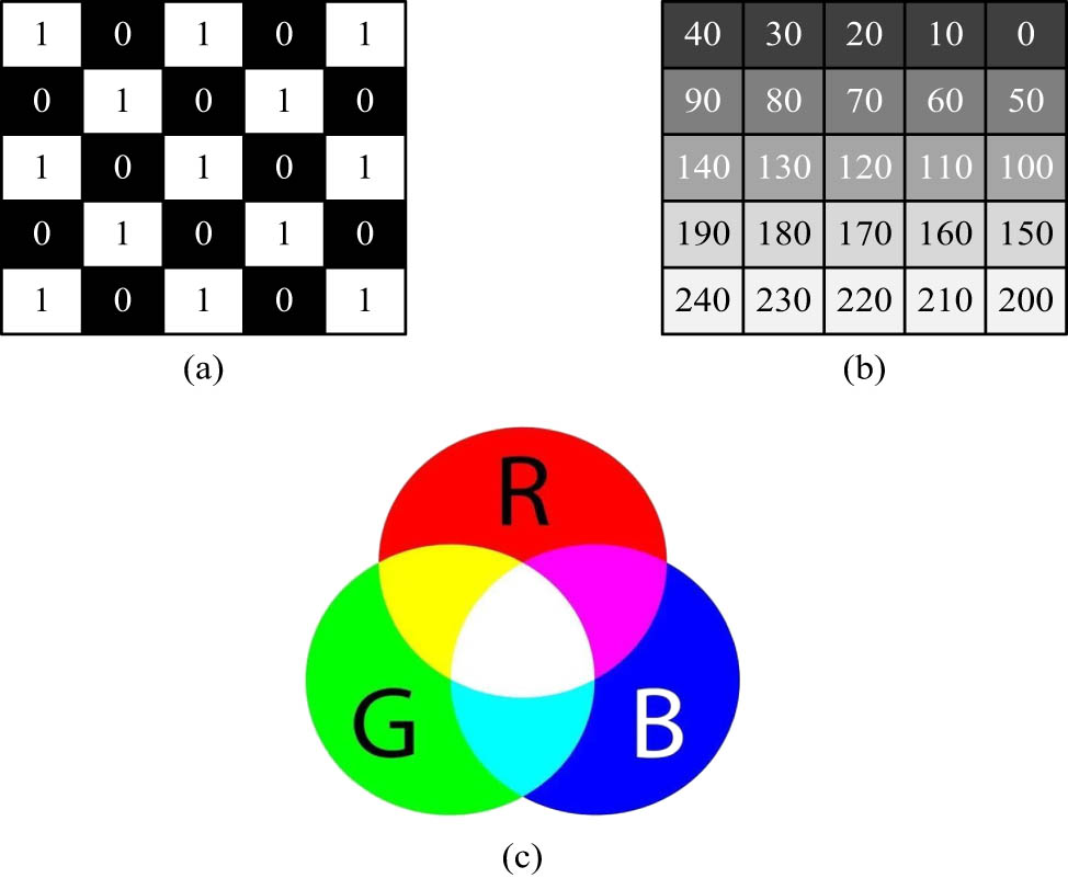
Classification chart of different digital 2D image types. (a) Schematic of a binary image. (b) Schematic of a grey scale image. (c) Colour image.

In Figure 2, there are a total of three different digital 2D image expressions, namely the binary image, grey scale image, and colour image. Among the three digital 2D image expressions, the grey level value of a pixel point in a binary image is represented by 1 and 0, where 1 represents white and 0 represents black. The grey level of a pixel in a grey scale image is represented by 1 to 255, with larger values indicating brighter brightness of the image. The pixel points in a colour image are made up of three colour quantities R, G, and B. When a fabric is converted into a digital 2D image in the form of a 3D fabric, the three different 2D image types mentioned above can be used to represent the grey values of the fabric image. The input value is the 2D image of the fabric collected under a D65 standard light source and the measured brightness data. Each fabric sample was measured randomly at five positions under a D65 standard light source, and the average brightness was recorded with a repeatability of ±0.5%. The luminance value was measured using a Konica Minolta CS-2000 spectrometer. To simulate standard conditions, the lighting was set to 45° and the sensor at 0° to the fabric surface. The specific operations were divided into three layers: graphic layer, shadow layer, and material layer for processing. In the graphic layer, based on the area ratio of yarn colour coverage, as shown in Eqs. (1) to (3), the warp and weft yarn regions were extracted through threshold segmentation, such as white warp/black weft.

(1) L pi = S j1 L j + S w1 L w .

In Eq. (1), L pi denotes the warp and weft brightness. S j1 and S w1 denote the area ratio of warp and weft yarns, respectively. Both are directly related to yarn density and coverage. L j and L w denote the measured brightness values of the warp and weft yarns of the fabric, respectively.

(2) L ti = S j 2 L j + S w 1 L w + S h 1 L h 1 .

In Eq. (2), L ti denotes the brightness of fabric projection. S h 1 and S j 2 denote the ratio of the projected area and the ratio of the area of the warp yarn outside the projection, respectively. L h 1 denotes the brightness value of the projection.

(3) L zi = S j 2 L j + S w 2 L w + S h 1 L h 1 + S h 2 L h 2 .

In Eq. (3), L zi denotes the brightness of the fabric’s dots. S h 2 and S w 2 denote the area ratio of the black weft and the area ratio of the weft other than the dots, respectively. L h 2 denotes the brightness value of dots. The current parameters are based on a benchmark experimental design, and in practical applications, the area ratio calculations, Eqs. (1)–(3), were adjusted according to the fabric structure, yarn twist, or dyeing differences. In the shadow layer, the shadow area ratio caused by the unevenness of the fabric surface was calculated using the projection geometry model, namely Eqs. (4) and (5).

(4) i = 1 , 2 , 3 … n .

In Eq. (4), n is the number of shading tissue library levels of the fabric colour card, and the range is indicated by i .

(5) S j = R w + ( n − 1 ) × ( R w / k ) R w 2 .

In Eq. (5), S j denotes the intentionally crafted warp area ratio. R w denotes the number of tissue cycles of the fabric. k denotes the growth rate of fabric tissue points. The optical parameters of the material layer were fitted through the reflectance curve of mulberry silk fibres, and the relevant parameters are shown in Table 1.

Table 1

Parameters of fabric colour cards

Parameter	Warp	Weft
Thread colour	White	Black
Wire density	22.2/24.4 dtex*2	22.2/24.4 dtex*2
Wire arrangement specification	1,100 pcs/10 cm	1,100 pcs/10 cm
Composition	Mulberry silk	Mulberry silk
Tissue point transition direction	Weft reinforcement	Weft reinforcement
Tissue structure	15 pcs 3f, 5f, 7f weft satinised	15 pcs 3f, 5f, 7f weft satinised

In Table 1, the thread density, colour, alignment density, composition, direction of transition of tissue points, and tissue structure of the radial and weft directions of the fabric swatch weaving yarns are given. Since the material and colour of the warp and weft yarns of the fabric will affect the brightness of the final fabric image, it needs to be strictly controlled according to the parameter specifications in Table 1.

To better predict the brightness values of fabric images, the images need to be layered, thereby better extracting the image features for analysis. Layered image photoreconstruction is a computer graphics and computer vision technique for analysing and reconstructing lighting information of a scene from images. The goal of hierarchical image photoreconstruction is to infer the lighting conditions of a scene from single or multiple images in order to better render or reconstruct a 3D scene. In conventional images, lighting information is mixed in colour and luminance and is difficult to separate out directly. The idea of hierarchical image light reconstruction is to separate the lighting information in an image from other factors such as surface colour and texture in order to better control the lighting conditions, and even to apply this information to other scenes or virtual worlds. The application of layered image light and shadow reconstruction techniques to fabric images can better extract the image layering features to achieve the prediction of fabric colour. The flowchart of the light and shadow reconstruction method for fabric images is shown in Figure 3.

Figure 3

Flowchart of fabric image light and shadow reconstruction method.

In Figure 3, it can be found that the light and shadow reconstruction method of fabric images is mainly composed of three parts: layering, assignment, and reconstruction. Image layering is done to obtain the warp and warp graphic layer, stereo shadow layer, and warp and warp material layer. Taking the warp and weft graphic layer as an example, it is divided into latitudinal area ratio and meridional area ratio, extracted as weft luminance and warp luminance, respectively. The final brightness summation achieves the fabric image. According to the results of fitting the reconstructed luminance value of the fabric image to the actual measured luminance value of the sample fabric, the contribution of the graphical characteristics of the layered image to the luminance of the fabric can be determined. By gradually analysing the brightness of each layer of the image and solving for each parameter value, the final brightness value can be obtained.

3.2 Design of an MR fabric brightness prediction model

MR is an extension of linear regression and is often used to solve situations involving multiple independent variables to more accurately predict the value of the dependent variable [18]. In the problem of fabric brightness prediction, since fabric brightness is related to a variety of factors such as material, fabric colour card, weaving process, image acquisition method, image processing method, etc., the study adopted MR to build a fabric brightness prediction model. The flow chart of the fabric brightness prediction model in MR is shown in Figure 4.

Figure 4

Flowchart for building the MR fabric brightness prediction model.

Figure 4 shows the flowchart of building the MR fabric brightness prediction model. As can be seen from Figure 4, in the process of building the prediction model, it is mainly divided into three parts. The first part is to design the fabric colour card and determine the weaving scheme and colour measurement scheme, so as to provide data for the subsequent prediction model. The second part is further acquisition and processing of data, in which the feature extraction of fabric images and the calculation of relevant parameters are completed. The third part is the construction of the prediction model based on the principle of MR. To control variables during the initial modelling stage and reduce the interference of fibre material differences in brightness prediction, the study chose Mulberry silk as the unified material for warp and weft yarns.

Fly value refers to the number of weft yarns skipped between two adjacent interlacing points in a satin weave structure. This value directly affects the smoothness of the fabric surface and the light reflection pattern [19]. For example, 3-fly (3f) means that the warp yarns float over 3 wefts before interlacing. A lower fly value can lead to more frequent interleaving, resulting in a diffuse matte appearance. A higher fly value will result in longer fluctuations, enhancing specular reflection and perceived brightness. After determining the fabric colour card, it is necessary to carry out the weaving process and collect the corresponding fabric image to extract the image features. The brightness value of the fabric can be obtained through weaving and colour measurement, and the areas of the white warp yarn graphic area, the black weft yarn graphic area, the miscellaneous point graphic area, and the projection graphic area can be obtained through image processing and data acquisition. The above-collected data were taken as independent variables, the fabric brightness was taken as the dependent variable, and the prediction model was established by combining MR. The MR modelling operation establishes a linear relationship through Eqs. (6)–(8). The fabric warp yarn graphic area rate reflects the brightness changes caused by weft yarn reinforcement. There is a linear relationship between the sum of fabric warp yarn graphic area rate, projected area rate, and the proportion of artisan warp yarn area S j , as shown in Eqs. (6) and (7) [20].

(6) S j = c × 1 c ( S j 2 + S h 1 ) .

In Eq. (6), c is a constant term. The constant term c combines the fly value with the density ratio, reflecting the linear effect of yarn arrangement on brightness. The specific calculation formula is shown in Eq. (7)

(7) c = q × P j × N tj P w × N tw .

In Eq. (7), q denotes the flight value. P j P w denotes the ratio of latitude and longitude densities. N tj N tw denotes the ratio of warp to weft density. In order to simplify the amount of calculation, the product of the area ratio of the spaghetti warp yarns S j and the constant term c is recorded as the area ratio of the fabric warp and weft graphics S j ∗ in this study. After the graphical eigenvalues of the layered fabric images were calculated according to the light and shadow reconstruction method, the multiple linear regression equation of fabric brightness was established as shown in Eq. (8).

(8) Y = b 0 + b 1 x 1 + b 2 x 2 + … + b m x m .

Here, Y denotes the predicted brightness of the fabric. b 0 denotes the predicted brightness of the fabric. b 1 and b 2 denote the coefficients of the monomials. b m denotes the coefficients of each monomial. x 1 , x 2 , and x m denote the indicators of each independent variable. m denotes the number of variables. The output value is the preliminary brightness prediction value and residual.

To test the performance of the regression prediction model, the coefficient of determination, mean absolute error (MAE), mean relative error (MRE), and root mean squared error (RMSE) were chosen as the testing indexes to test the performance of the model.

(9) R 2 = 1 − ∑ i = 1 n ( y i − y ˆ i ) ∑ i = 1 n ( y i − y ¯ ) .

In Eq. (9), R 2 denotes the coefficient of determination, which is used to detect the degree of linear fit between the independent variable and the dependent variable. The closer the value of the coefficient is to 1, the better the fit of the model. y i denotes the actual measured value of fabric brightness, and its average value is denoted as y ¯ . y ˆ i denotes the predicted value of fabric brightness.

(10) MAE = 1 n ∑ i = 1 n ∣ y i − y ˆ i ∣ 2 .

In Eq. (10), MAE denotes the average absolute error, which is used to reflect the actual situation of the prediction value error.

(11) MRE = 1 n ∑ i = 1 n ∣ y i − y ˆ i ∣ y i .

In Eq. (11), MRE denotes the average relative error, which is used to compare the degree of confidence in the prediction results of each type of model.

(12) RMSE = ∑ i = 1 n ( y i − y ˆ i ) 2 n .

In Eq. (12), RMSE denotes the root mean square error, which is used to measure the deviation between the predicted and actual values.

3.3 Design of an MR fabric brightness prediction model based on BPNN optimisation

Since the regression prediction model is prone to underfitting after multiple trainings and the BP neural network (BPNN) in machine learning has a better nonlinear fitting performance, the study will combine the BPNN to further optimise the above MR model. The regression model was used to deal with the linear features in the data, the BPNN model was used to deal with the nonlinear features in the data, and finally the two models were combined to obtain the final brightness prediction model.

Since the three-layer BPNN has the advantages of a stable structure that can approximate any functional relationship between the data and achieve multi-dimensional mapping, a three-layer structure was chosen to build the BPNN model. In order to further improve the prediction accuracy of the model, the study uses Eq. (13) to determine the number of neurons in the hidden layer.

(13) h = u + o + α .

In Eq. (13), h , u , and o denote the number of nodes in the implicit layer, input layer, and output layer, respectively. α denotes the adjustment coefficient. In h , the specific numbers of u and o need to be decided by the final optimisation result of the model and takes the value of 1. The Tanh function was chosen as the transfer function from the input layer to the implied layer, and the tansig function was chosen as the transfer function from the implied layer to the output layer, so as to improve the convergence speed of the model. The flowchart of the brightness regression prediction model combined with the BPNN is shown in Figure 5.

Figure 5

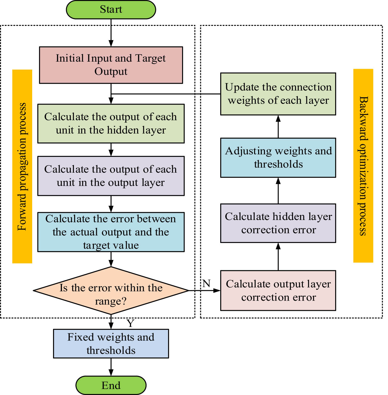
Flow chart of BPNN-MR model prediction.

The flowchart of the operation of the brightness regression prediction model incorporating the BPNN is shown in Figure 5. After the initial input and target output, calculate the output of each unit in the hidden layer and output layer. Then, calculate the error between the actual output and the target value. If the error is within the range, the loop ends with fixed weights and thresholds. If not, calculate the correction error of the hidden layer and output layer. Adjust the weights and thresholds and update the connection weights of each layer. Recalculate the output of each unit in the hidden layer and output layer and loop again. The result after MR prediction was used as the input of the BPNN model for optimisation, and the BPNN learned the implicit mapping relationship between the weave complexity and brightness. The final brightness prediction model was obtained through multiple trainings and is denoted as BPNN-MR. The BPNN part of the BPNN-MR was used to process the nonlinear data in the fabric image, and the MR model was used to process the relationship between the linear data, and finally the hybrid model BPNN-MR was used for the prediction of the fabric brightness value.

4 BPNN-MR fabric brightness prediction model performance testing and application effect analysis

In this study, the coefficient of determination, the MAE, the MRE, and the RMSE were selected as the detection indexes to test the performance of different MR models in the same dataset, so as to verify the performance of BPNN-MR. In addition, two different specifications of fabric upholstery fabrics were selected to test the brightness prediction effect of BPNN-MR in practical applications, and it was found that the predicted brightness values of the model were almost the same as the actual values, which could predict the brightness of fabrics well.

4.1 Performance test of the BPNN-MR fabric brightness prediction model

In order to verify the robustness of the BPNN-MR model for brightness prediction in different fabric structures, the dataset was divided into three parts: the training set contains 3f and 7f colour card samples, accounting for 70% of the total data. The validation set consisted of 15% of the 5f colour card samples and was used for tuning hyperparameters. The test set also consisted of 15% of the 5f colour card samples, which was used to simulate the prediction situation of unknown samples. To further test the performance of the BPNN-MR fabric brightness prediction model, it is first necessary to calculate the mean and standard deviation of the brightness corresponding to different fly values in the colour cards to determine whether different fly values affect the fabric brightness. The mean and standard deviation of 15 cards with 3f, 5f, and 7f values in the colour chart were analysed using one-way ANOVA, as shown in Table 2.

Table 2

Mean and standard deviation of luminance of fabric swatches with different fly values

Fabric colour Card fly values	Mean value	Standard deviation	p value (vs 3f)	p value (vs 5f)
3f	48.56 ± 12.61	12.94 ± 8.25	—	—
5f	50.21 ± 10.28	15.18 ± 10.11	0.043	—
7f	44.35 ± 11.74	13.07 ± 9.69	0.021	0.003

In Table 2, the luminance mean and standard deviation of the fabric swatches with different fly values are given. According to the data in Table 2, it can be seen that the overall luminance mean and standard deviation of the colour cards increased and then decreased with the increase of fabric fly values. The cover factor measured the percentage of fabric area covered by yarn, while the fly value captured the structural periodicity of light scattering points in satin fabrics. Choosing the fly value as the brightness prediction value for satin fabric is more reliable, while cover factor is more suitable for plain weave fabric. There was a significant difference in brightness between 5f and 3f (p = 0.043), and there were significant differences between 7f and both 3f and 5f values (p <0.05). The brightness of the 7f group was significantly lower than the other two groups, which may be related to the long floating line reflection characteristics.

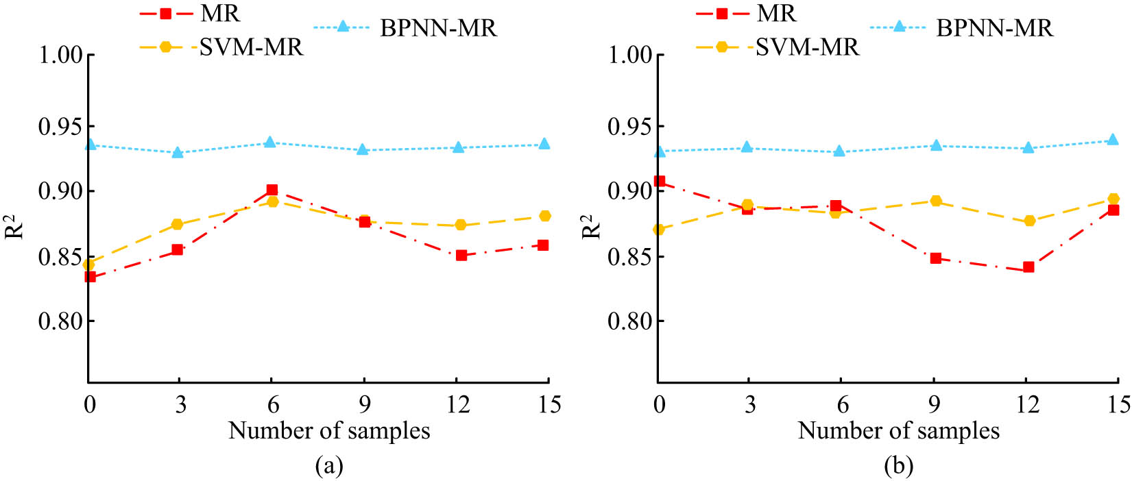
In order to better test the prediction performance of each model for fabric brightness, the study chose the 5f value card in the colour card as the test sample set and 3f and 7f value cards as the training sample sets, and tested the R 2 value, the MAE value, the MRE value, and the RMSE value of the three different regression models under the same dataset, respectively. The R 2 values of the three regression models in the training dataset and the test dataset were first compared, as shown in Figure 6.

Figure 6

Values of coefficient of determination for different prediction models. (a) Magnitude of the coefficient of determination values for the three models in the training dataset. (b) Magnitude of coefficient of determination values for the three models in the test dataset.

In Figure 6, the three prediction models are multiple regression (MR), support vector machine-multiple regression (SVM-MR) under optimisation, and the BPNN proposed in this research. Figure 6(a) and (b) presents the R 2 values of the three prediction models on the training dataset and test dataset, respectively. From Figure 6(a) and (b), it can be seen that the R 2 values of the three prediction models changed with the change of the training sample data. Among them, the R 2 value of the BPNN-MR model is stable around 0.94 in both the training dataset and the test dataset, while the R 2 value of the MR model and the SVM-MR model has a large fluctuation. Among them, the R 2 of the MR model is less than 0.90. In contrast, the BPNN hidden layer in the BPNN-MR model reconstructs the features of high-order nonlinearities that are not captured by MR.

Figure 7(a) and (b) presents the RMSE values of the three prediction models in the training dataset and test dataset, respectively. As can be seen from Figure 7(a), the average RMSE values of the three models BPNN-MR, SVM-MR, and MR in the training dataset are around 3.8, 5.7, and 7.1, respectively. From Figure 7(b), the average RMSE values of the three models BPNN-MR, SVM-MR, and MR in the test dataset are around 3.9, 5.9, and 7.5, respectively. Comparing the RMSE values of the three models, it can be found that the average error value of BPNN-MR is smaller, which indicates that the model has a better prediction effect. In order to further represent the training error situation of the model, the MAE value and MRE value of the two models, BPNN-MR and SVM-MR, are given in Figure 8.

Figure 7

RMSE values for different prediction models. (a) RMSE values of the three models in the training dataset. (b) RMSE values for the three models in the test dataset.

Figure 8

MAE and MRE values for different prediction models. (a) Relative and absolute errors under SVM-MR prediction modelling. (b) Relative and absolute errors under BPNN-MR prediction modelling.

Figure 8(a) and (b) presents the MAE and MRE values of the SVM-MR and BPNN-MR models in the test dataset, respectively. As can be seen from Figure 8(a), the MAE values and MRE values of the SVM-MR model have a large error. Taking sample 1 as an example, the MAE and MRE values of this sample in the SVM-MR model are 4.2 and 11.8, respectively. On the contrary, as can be seen from Figure 8(b), the MAE and MRE values of the BPNN-MR model are closer. Taking sample 1 as an example, the MAE and MRE values of this sample in the BPNN-MR model are 6.1 and 7.9, respectively. In summary, it can be seen that the MAE and MRE values in the BPNN-MR model are much closer to each other, which indicates that the model has a much smaller error during the training process, and its prediction is much closer to the actual situation. In the BPNN-MR model, the estimated coefficient of the intercept term is 2.3, with a standard error of 0.5, and P <0.001, statistically significant. The results of MR prediction have a significant impact on the output of the model, which also verifies the importance of the MR model in predicting brightness values.

4.2 Analysis of the effect of applying the BPNN-MR fabric brightness prediction model

The performance of the above three regression models was tested through the detection indexes of the coefficient of determination R 2 , the MAE, the MRE, and the RMSE, and the BPNN-MR model was found to have the best performance. In order to further illustrate the advantages of the BPNN-MR model in the prediction of fabric brightness, two fabric decorative fabrics were selected for the study to test the effect of practical application. The luminance test results of the two fabric decorative fabrics in the BPNN-MR model are shown in Table 3.

Table 3

Brightness test results of two upholstery fabrics in BPNN-MR modelling

Decorative fabric type	Organisation number	Actual luminance value	Tested luminance value
First type of decorative fabric	1	35.45	34.25
	2	41.26	40.16
	3	44.21	45.26
	4	38.19	37.75
	5	34.82	35.09
	6	27.11	27.51
	7	48.37	50.16
	8	28.15	29.34
	9	23.62	24.81
	10	39.02	40.05
Second type of decorative fabric	1	68.23	70.11
	2	73.54	72.74
	3	66.15	65.54
	4	84.10	85.09
	5	67.64	67.95
	6	69.21	68.08
	7	74.08	75.23
	8	77.25	75.18
	9	79.63	80.17
	10	81.42	81.56

In Table 3, ten tissue colour blocks were randomly selected from two kinds of decorative fabrics to be labelled in order, and their brightness values were examined. As can be seen from Table 3, the actual luminance values of the first decorative fabric are between 20 and 50, while the actual luminance values of the second decorative fabric are between 60 and 90. The predicted luminance values in the BPNN-MR model are basically the same as the actual luminance values, and the data difference between the predicted values and the actual values is basically within 3°. For the first type of decorative fabric, the BPNN-MR prediction error is only 1.21 ± 0.89 brightness units, which is suitable for heavy fabrics with a high proportion of shadow layers, such as curtain fabrics. For the second type of decorative fabric, the model successfully captures the mirror reflection characteristics of 7f satin pattern, which is suitable for strong light environments such as car interiors.

The predicted brightness values of the two models, BPNN-MR and SVM-MR, for different tissue colour blocks in the two fabric upholstery fabrics are shown in Figure 9. As can be seen from Figure 9(a), the predicted and actual values of each tissue colour block in the BPNN-MR model are basically the same. As the organisation number gradually increases, the trend of luminance value changes is basically similar between the two. From Figure 9(b), it can be seen that in the SVM-MR model, there is a discrepancy between the predicted and actual values of each tissue colour block. The maximum difference between the two is 22. In contrast, BPNN-MR has a better predictive effect on fabric brightness than SVM-MR. This is because the multi-layer structure of BPNN enables it to extract and optimise data features layer by layer, thereby better fitting the changing trend of brightness values. This enables the BPNN-MR model to more accurately reflect the actual brightness of colour blocks in fabric interior organisation.

Figure 9

Predicted and actual values of brightness of each fabric organisation in different prediction models. (a) Predicted and actual brightness values of the BPNN-MR model. (b) Predicted and actual brightness values of the SVM-MR model.

The satisfaction of merchants and users for the three brightness prediction models is shown in Figure 10. From Figure 10, it can be seen that the user and merchant satisfaction values are 79.2 and 82.0 for the MR model, 88.4 and 91.5 for the SVM-MR model, and 95.3 and 97.8 for the BPNN-MR model. In conclusion, the BPNN-MR model is able to obtain higher user satisfaction and merchant satisfaction.

Figure 10

Merchant and user satisfaction with different prediction models.

5 Conclusions

To achieve diversity in fabric design, this study innovatively constructed a BPNN-MR fabric brightness prediction model by combining light and shadow reconstruction theory, MR prediction model, and BPNN. The results indicate that the BPNN-MR model controls the fabric brightness prediction error within 3° through light and shadow layering technology. The R 2 of the BPNN-MR model in the training and testing sets is approximately 0.94. The RMSE value in the BPNN-MR model is much lower than that of MR and SVM-MR, with average RMSE values of 3.8 and 3.9 on the training and testing sets, respectively. The user satisfaction and business satisfaction values of the BPNN-MR model are as high as 95.3 and 97.8, respectively, while those of the MR model are 79.2 and 82.0, respectively. In summary, the BPNN-MR model combines the process interpretability of the MR model with the nonlinear fitting ability of BPNN. However, this study only focused on brightness features and did not consider the influence of other tissue parameters. The future direction can be extended to multimodal fabric features, such as joint prediction of texture and glossiness to improve the feature recognition effect of fabric images.

Funding information: This study was supported by the 2021 Higher Education Teaching Reform Project of Henan Province “Research and Practice of Personalized Skill Talent Training Mode based on Skills Competition” (Project No.: 2021SJGLX736).
Author contributions: The author has accepted responsibility for the entire content of this manuscript and approved its submission.
Conflict of interest: The author states no conflict of interest.
Data availability statement: All data generated or analysed during this study are included in this article and supplementary material.

References

[1] Wang P, Li Q, Shen D, Liu Y. High-dimensional factor regression for heterogeneous subpopulations. Stat Sin. 2023;33(1):27–53. 10.5705/ss.202020.0145.Search in Google Scholar PubMed PubMed Central

[2] Banik A, Dutta S, Bandyopadhyay TK, Biswal SK. Prediction of maximum permeate flux (%) of disc membrane using response surface methodology (RSM). Can J Civ Eng. 2019;46(4):299–307. 10.1139/cjce-2018-0007.Search in Google Scholar

[3] Yoon D, Kim K, Dong HC, Lee M, Im J, Cho D, et al. Development of model output statistics based on the least absolute shrinkage and selection operator regression for forecasting next-day maximum temperature in South Korea. Q J R Meteorol Soc. 2022;148(745):1929–44. 10.1002/qj.4286.Search in Google Scholar

[4] Sun X, Cinar A, Yu X, Rashid M, Liu J. Kernel-regularized latent-variable regression models for dynamic processes. Ind & Eng Chem Res. 2022;61(17):5914–26. 10.1021/acs.iecr.1c04739.Search in Google Scholar

[5] Farias-Basulto GA, Reyes-Figueroa P, Ulbrich C, Szyszka B, Schlatmann R, Klenk R. Validation of a multiple linear regression model for CIGSSe photovoltaic module performance and Pmpp prediction. Sol Energy. 2020;208(9):859–65. 10.1016/j.solener.2020.08.040.Search in Google Scholar

[6] Dharma F, Shabrina S, Noviana A, Tahir M, Hendrastuty N, Wahyono W. Prediction of Indonesian inflation rate using regression model based on genetic algorithms. J Online Inform. 2020;5(1):45–52. 10.15575/JOIN.V5I1.532.Search in Google Scholar

[7] Loftis C, Yuan K, Zhao Y, Hu M, Hu JJ. Lattice thermal conductivity prediction using symbolic regression and machine learning. J Phys Chem A. 2020;125(1):435–50. 10.1021/ACS.JPCA.0C08103.Search in Google Scholar

[8] Wang J, Qu H. Analysis of regression prediction model of competitive sports based on SVM and artificial intelligence. J Intell Fuzzy Syst. 2020;39(4):5859–69.10.3233/JIFS-189061Search in Google Scholar

[9] Bing DU, Duan Y, Zhang H, Tao X, Yue W, Cong RU. Collaborative image compression and classification with multi-task learning for visual Internet of Things. Chin J Aeronaut. 2022;35(5):390–9.10.1016/j.cja.2021.10.003Search in Google Scholar

[10] Yuan Q, Yao LF, Tang JW, Ma ZW, Mou JY, Wen XR, et al. Rapid discrimination and ratio quantification of mixed antibiotics in aqueous solution through integrative analysis of SERS spectra via CNN combined with NN-EN model. J Adv Res. 2025;69:61–74. 10.1016/j.jare.2024.03.016.Search in Google Scholar PubMed PubMed Central

[11] Yeoh PSQ, Lai KW, Goh SL, Hasikin K, Wu X, Li P. Transfer learning-assisted 3D deep learning models for knee osteoarthritis detection: Data from the osteoarthritis initiative. Front Bioeng Biotechnol. 2023;11(1):10. 10.3389/fbioe.2023.1164655.Search in Google Scholar PubMed PubMed Central

[12] Deng XQ, Chen BL, Luo WQ, Luo D. Universal image steganalysis based on convolutional neural network with global covariance pooling. J Computer Sci Technol. 2022;37(5):1134–45. 10.1007/s11390-021-0572-0.Search in Google Scholar

[13] Teoh JR, Hasikin K, Lai KW, Wu X, Li C. Enhancing early breast cancer diagnosis through automated microcalcification detection using an optimized ensemble deep learning framework. PeerJ Computer Sci. 2024;10:e2082. 10.7717/peerj-cs.2082.Search in Google Scholar PubMed PubMed Central

[14] Cao H, Cui R, Liu W, Ma T, Zhang Z, Shen C, et al. Dual mass MEMS gyroscope temperature drift compensation based on TFPF-MEA-BP algorithm. Sens Rev Sens Rev. 2021;41(2):162–75. 10.1108/SR-09-2020-0205.Search in Google Scholar

[15] Guo Y, Mustafaoglu Z, Koundal D. Spam detection using bidirectional transformers and machine learning classifier algorithms. J Comput Cognit Eng. 2022;2(1):5–9.10.47852/bonviewJCCE2202192Search in Google Scholar

[16] Debebe E, Birhan T, Shitahun Y, Belay M, Adelahu N. Effect of jacquard structures on the tensile strength property of weft knitted fabrics. J Des Text. 2024;3(1):30–45.Search in Google Scholar

[17] He W, Song B, Zhang N, Xiang J, Pan R. Modeling and realization of image-based garment texture transfer. Vis Computer. 2024;40(9):6063–79. 10.1007/s00371-023-03153-w.Search in Google Scholar

[18] Xu KL, Guo J. A new test for multiple predictive regression. J Financ Econom. 2024;22(1):119–56.10.1093/jjfinec/nbac030Search in Google Scholar

[19] Wang Q, Xi H, Deng F, Cheng M, Buja G. Design and analysis of genetic algorithm and BP neural network based PID control for boost converter applied in renewable power generations. IET Renew Power Gener. 2022;16(7):1336–44. 10.1049/rpg2.12320.Search in Google Scholar

[20] Meng S, Pan R, Gao W, Yan B, Peng Y. Automatic recognition of woven fabric structural parameters: A review. Artif Intell Rev. 2022;55(8):6345–87. 10.1007/s10462-022-10156-x.Search in Google Scholar

Received: 2023-11-01

Revised: 2025-07-14

Accepted: 2025-07-25

Published Online: 2025-09-08

This work is licensed under the Creative Commons Attribution 4.0 International License.

Articles in the same Issue

https://doi.org/10.1515/nleng-2025-0172

Keywords for this article

photoreconstruction; fabric; image; multiple regression; prediction; brightness

Creative Commons

BY 4.0