Real-time force/position control of soft growing robots: A data-driven model predictive approach
-
Abdonoor Kalibala
 ,
Ayman A. Nada
,
Ayman A. Nada

Abstract
Vine robots represent a novel class of soft robots that achieve mobility through tip extension, a mechanism inspired by the natural growth processes of vine plants. This unique movement strategy enables effective navigation in constrained and cluttered environments, offering significant advantages over conventional robotic systems. However, the continuum nature and inherent compliance of vine robots introduce complex modeling and control challenges. Deep learning offer a powerful alternative for modeling systems with such complex dynamics. In this article, we present a data-driven dynamic model for a pressure-driven everting vine robot, utilizing a deep neural network (DNN)-based discrete-time dynamic model. This model was integrated into a model predictive control (MPC) framework, and a comparative analysis was conducted against the MPC framework using a nonlinear first-principle model of the vine robot. The results demonstrate that the DNN-MPC framework offers a better control performance and significantly improved computational efficiency compared to the MPC based on the nonlinear first-principles model. The DNN-MPC reduced computation time by a factor of 11, making it highly viable for real-time control applications.
1 Introduction
The animal kingdom, a rich source of inspiration for science and engineering, has long influenced the development of robotics. Recently, researchers have turned their attention to the plant kingdom, creating robots that emulate plant properties such as growth, energy efficiency, sustainability, and adaptability to unknown environments. Plants provide a vast array of mechanisms and materials, from roots to leaves and seeds to flowers, offering abundant bio-inspiration that can be harnessed to develop sustainable and efficient technologies for solving complex problems [1]. Unlike animals, which primarily rely on locomotion to navigate their environments [2], plants utilize growth as their primary means of movement. This unique strategy, characterized by tip extension toward stimuli such as sunlight, operates at a slower rate and is a hallmark of the plant kingdom [3,4]. This type of growth-driven movement can be observed across various scales in nature, including in neurons [5], pollen tubes [6], trailing vines searching for support, and climbing plants that develop tendrils [7,8]. Recently, there has been a significant progress in replicating this form of movement in robotic systems inspired by vine plants. These robots, often referred to as “vine robots” or “growing robots,” aim to mimic the growth behavior of plants to navigate and interact with their surroundings in a manner similar to natural vines.
Replicating growth in robotic systems is archived by employing an ingenious method called pressure-driven eversion of flexible thin-walled material. This technique involves turning a thin-walled membrane inside out. When pressurized, the internal pressure forces the material to extend from the core of the existing body, causing it to evert at the tip and elongate. Robots that utilize this mechanism are known as everting vine robots. These robots offer several advantages over traditional rigid robots: there is no relative movement between the body and the environment since only the tip moves relative to the ground, reducing energy dissipation due to minimal friction and inertia. The tip’s movement creates a three-dimensional (3D) structure, which can be used to deliver payloads, transfer force, and form structures for various applications [9]. Everting vine robots are especially useful in navigating unstructured and space-constrained environments [10,11]. The application areas of vine robots are diverse and include minimally invasive surgery, surveillance and monitoring, soft burrowing devices, soft artificial muscles, and reconfigurable antennas [12–15].
However, the continuum nature and inherent compliance of the vine robot introduce a new set of modeling and control challenges compared to traditional rigid manipulators [16,17]. Modeling the dynamic behavior of vine robots presents significant mathematical complexity due to the inherent nonlinearities typically exhibited in soft robots. The air takes time to fill the pressure chamber, causing a delay in response to input pressure. In addition, the dynamic nature of the compressed air and the arbitrary geometry of the vine robot introduce further nonlinearities. As a result, first-principle models often fail to capture these dynamics accurately due to their simplifications. The piecewise kinematic models and kinematic-based controllers [18] for vine robots are suitable in scenarios where fast response times are not critical. However, these models do not explicitly capture the influence of forces, moments, and interactions with the external environment on the robot’s motion, limiting their applicability in dynamic and reactive tasks. Alternative modeling approaches, such as the simulation open framework architecture (SOFA) [19], which is based on the finite element method (FEM), have also been explored. While FEM-based models offer a high degree of accuracy in capturing complex deformations, they suffer from significant computational costs and lack the capability to be easily transformed into mathematical models that are compatible with model-based controllers, thus limiting their use in real-time applications. These modelling challenges also affects the control strategies employed to control the vine robot.
Model-based control strategies, such as model predictive control (MPC), are employed to simultaneously predict and control the growth and steering behavior of the everting vine robot in free space, utilizing either kinematic or dynamic models [18,20]. MPC predicts the future behavior of the controlled system by solving a constrained optimization problem within a finite time horizon at each time step [21]. The widespread use of MPC in robotics is attributed to its ability to control complex nonlinear systems with constraints and uncertainty, a hallmark feature of soft robotic systems that often confounds classical linear control methods [21,22]. The initial challenge in applying MPC lies in developing a dynamic model that accurately and efficiently describes the system’s behavior while being suitable for real-time control applications. This requires a thorough understanding of the system dynamics to create models that can predict future states and control actions effectively. In addition, the computational efficiency of the optimization process is crucial to ensure that the control actions can be computed within the time constraints required by real-time applications.
Developing a mathematical model for an everting vine robot that balances computational efficiency with sufficient accuracy is crucial for capturing the dynamics of this soft, flexible robot and for optimizing its design and control. The continuum nature, inherent compliance, and pneumatic actuation of the vine robot closely align with the core principles of soft robotic systems, which are defined by their flexibility and adaptability. State-of-the-art modeling techniques in soft robotics, such as the piecewise constant curvature approach, can be further enhanced by incorporating growth dynamics inspired by plant tip extension. This integration would enable a more comprehensive representation of the vine robot’s motion, capturing both its unique growth-driven locomotion and its interaction with the environment, thereby broadening the applicability and flexibility of current soft robotics models. Only a limited number of studies have ventured into developing a dynamic model for everting vine robots to characterize their behavior in response to environmental interactions and actuator inputs, primarily due to the inherent complexity of such systems. In the study by Blumenschein et al. [23], a quasi-static force balance model for a pressure-driven everting vine robot was developed. This model focuses on the equilibrium of forces, disregarding system inertia, and links the driving force generated by internal pressure to the yield force and a term dependent on velocity. Similarly, Blumenschein et al. [24] presented a quasi-static model for a novel growing soft-continuum robot. This model integrates a kinematic framework with a quasi-static approach to precisely control the position of the end effector within the task space. In the study by Haggerty et al. [10], a detailed mathematical model was developed to describe the behavior of vine robots interacting with their environment in both unconstrained and constrained scenarios. This model accounts for axial and transverse buckling modes as the robot grows into obstacles, based on a quasi-static equilibrium framework for vine robots traveling at an average speed of less than 0.05 m/s and a path length of less than 5 m. Similarly, Naclerio et al. [13] modified a quasi-static model to consider the external opposing force of dry sand, where the soft burrowing device operates. This device utilizes tip-extension, inspired by plant root growth, and incorporates granular air-fluidization by channeling air through the backbone core.
Physics-based model for a miniature steerable soft growing robot, employing the SOFA to simulate growth, steering, external loading, and pressure stiffening was developed in the study by Wu et al. [19]. Despite its detailed simulations, this model is computationally intensive and unsuitable for real-time control. In contrast, Jitosho et al. [25] introduced a dynamic simulator for soft growing robots using pseudo-rigid-body kinematics with contact constraints to examine vine robot interactions with the environment. However, this model does not consider continuous length changes, it is restricted to planar motion, and its performance is limited by the number of discrete rigid bodies included. Despite significant efforts in developing dynamic models for pressure-driven everting vine robots to describe their behavior, it remains prohibitively challenging to create a parsimonious and computationally efficient model suitable for real-time control. The inherent complexities of these robots, including their nonlinear dynamics and interactions with the environment, pose substantial obstacles to achieving both accuracy and computational tractability in real-time applications.
Data-driven modeling, employing machine learning techniques, presents a novel approach to characterizing complex systems, including the use of deep learning [26]. Deep learning, a subset of artificial intelligence and machine learning, utilizes multilayer neural networks to identify patterns within data, effectively correlating input features with target outcomes. The confluence of big data, advanced algorithms in machine learning, and advancements in computational hardware are fueling a new paradigm in modeling and control of complex systems, resulting in watershed moment in the modern dynamical systems and transformative progress in data-driven dynamic systems of soft robots [27]. Recent works have demonstrated the effectiveness of deep neural networks (DNN) in modeling complex dynamic systems of soft robots. In the study by Cespedes et al. [28], a DNN was used to estimate the dynamic model of a soft robotic laparoscope using data sampled at fixed time steps for random inputs from the system. Similarly, in the study by Hyatt et al. [29], a neural network obtained from data-driven principles was used as a surrogate model in a MPC. A neural network-based dynamic model for a soft robot with symmetrical chambers, which was used to develop a MPC to control the motion and track the desired trajectory of the robot, was developed by Li et al. [11]. These studies demonstrate the potential of combining neural network-based dynamic models with MPC, offering improved computational efficiency and performance compared to traditional analytical models for soft robots.
In this work, we present a data-driven dynamic model for a pressure-driven everting vine robot, utilizing advanced deep learning techniques. A nonlinear first principles model of the everting vine robot was developed, and a DNN was employed to approximate the nonlinear discrete-time dynamics using data from nonlinear simulations of the proposed analytical model of the vine robot. The DNN-based dynamic model was then integrated into a MPC framework to enhance the data-driven control of the vine robot, improving computational efficiency for real-time applications. The deep learning model was rigorously validated against the first principles model by comparing the computation time required to determine optimal control actions. Furthermore, we performed k-fold validation to assess the model’s generalization performance, ensuring robustness across different datasets.
The model was successfully incorporated into the MPC framework with additional constraints and bounds to ensure operation within the physical limitations of the actuators and the feasible region of the state space. Simulation results demonstrated significantly improved performance in trajectory tracking capabilities, point stabilization, and obstacle avoidance, highlighting the potential of combining deep learning with MPC for advanced control of soft robots. In addition, the computation time of the MPC optimizer reduced significantly with DNN-based dynamic model compared to the nonlinear first principles model.
The key contributions of this article can be summarized as follows:
Development of a DNN architecture for dynamic modeling of a pressure-driven everting vine robot, utilizing data from a nonlinear first principles model.
Designing a MPC that employs the neural network (NN)-based dynamic model, which is computationally efficient, to control the growth and direction of the vine robot.
Formulation of a flexible first-principles model of the everting vine robot that accurately represents its dynamic behavior.
Contribution to the literature by proposing a versatile model applicable to any pneumatic growing robot, irrespective of the steering mechanism used.
Benchmarking and validation of the DNN-based dynamic model against the first principles model by evaluating the computation time required by the MPC optimizer to find the optimal control actions under given constraints, bounds, and uncertainties.
The remainder of this article is structured as follows: Section 2 presents the basic structure of the everting vine robot and its kinematic analysis in Cartesian space. The dynamic model, encompassing both the growth and steering behaviors, is introduced in Section 3. Section 4 discusses the stresses experienced by the growing robot during operation. The data-driven dynamic model is detailed in Section 5, followed by the development of the MPC framework in Section 6. Simulation results are presented in Section 7, and finally, conclusions are drawn in Section 8.
2 Kinematics of vine robots
2.1 Structure description
The structural design of the vine-growing robot examined in this study is illustrated in Figure 1. The robot comprises several key components: a pressure chamber, a spool, a flexible tube, and a steering mechanism that enables control of the robot’s tip local roll and yaw angles. The flexible tube, typically made from thin-walled low-density polyethylene, is sealed at one end and inverted, passing through the center of the existing tube before being rolled onto the spool. The open end is securely attached to the nozzle of the pressure chamber. When pressurized air from a compressor is introduced into the pressure chamber, the internal pressure propels the material through the robot’s body, causing it to evert at the tip and extend in length. This process is referred to as growth.
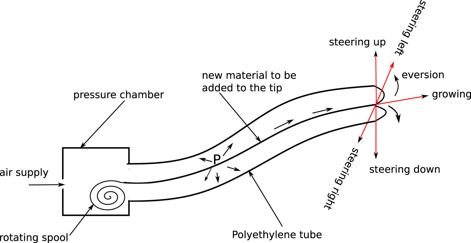
Schematic diagram of vine growing robot depicting its structure.
The servomotor, attached to the spool, manages the feeding of material necessary for the robot’s growth and retracts the material after task completion. While some studies use a servomotor to control the robot’s elongation, in this research, the servomotor is employed solely for two purposes: to feed the material required for growth without causing tension in the “tail” – the material that travels within the robot’s body – and to retract the material after the task is completed.
The steering system typically employs distributed strain actuation, using flexible actuators evenly spaced along the robot’s backbone to achieve distributed strain. Alternatively, it may use concentrated strain actuation, where actuators are placed at specific intervals along the robot’s length. Regardless of the approach, the primary purpose of the steering mechanism is to control the robot’s growth direction by adjusting the local roll and yaw angles. This is accomplished through asymmetric growth, which creates a length differential on either side of the robot’s body, mimicking how a vine bends due to uneven cell growth on its sides.
2.2 Kinematic analysis
To determine the tip’s position and orientation of the soft growing robot, it is essential to establish its kinematics within the chosen configuration space. Various methods such as piecewise constant curvature [18,20,30] and the classical Denavit–Hartenberg (D-H) coordinate system [11] have been utilized to elucidate the kinematics of vine robots. The piecewise constant curvature approach is particularly favored for modeling a broad array of continuum robots due to its analytical elegance and the capability to decompose kinematics into two distinct mappings: from actuator space to configuration space and from configuration space to task space [16]. This method is especially accurate for soft robots with a single curvature and actuators distributed along their backbone, proving effective when gravitational effects and external loads are negligible [31]. However, it is less suitable for soft robots with minimal bending curvatures [32], and the constant curvature assumption becomes unreliable at longer lengths [33].
Conversely, the classical D-H coordinate approach, while providing a homogeneous transformation matrix, relies on parameters that are difficult to measure directly in real-time settings. Therefore, this study adopts a comprehensive and general approach to model the kinematics of the growing robot, integrating the strengths of both methods to accurately capture the robot’s kinematic behavior in various conditions.
Figure 2 illustrates the detailed kinematic modeling of a vine-growing robot in free space. The global frame
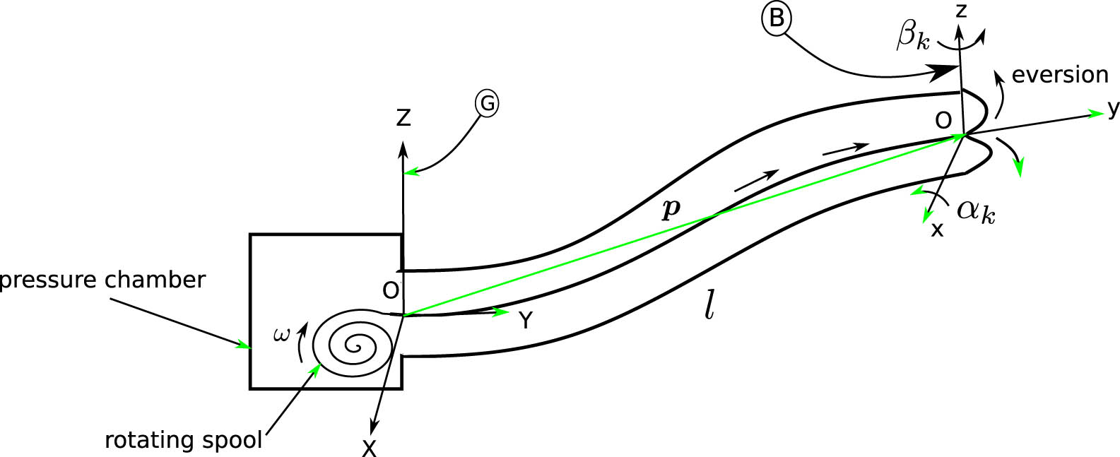
Schematic diagram of the kinematic model of the vine robot.
The spool, rotating at an angular velocity
where
and
In this study, the final orientation of the body frame
Let
For
However, if
The rate at which the everted length
To prevent tension in the tail, the rate at which the spool feeds the robot’s body during growth must be at least equal to the rate at which material is added at the robot’s tip. This ensures that the material supply keeps pace with the extension demands. This constraint is crucial to avoid buckling caused by the force applied at the tip due to tension in the tail and to simplify the dynamic model. Consequently, the velocity of the tip is controlled solely by internal air pressure. Maintaining this balance is essential for ensuring smooth and uninterrupted growth, as well as preventing mechanical failure. The mathematical relationship governing this balance is expressed as follows:
where
3 Dynamic modeling
This section presents a dynamic model for the growing vine robot, designed to be both computationally efficient and suitable for real-time implementation. This model aids in the development and synthesis of closed-loop controllers. In this study, we employ a lumped parameter model, which simplifies the system by assuming a single-point mass at the tip of the soft growing robot. This approach is chosen for its effectiveness in capturing the dynamics of mixed systems across various domains and for its ability to describe system behavior through computationally efficient ordinary differential equations. Furthermore, the lumped parameter model facilitates seamless integration with control algorithms and accelerates the rapid testing and iteration of different models, enhancing the overall development process.
3.1 The growth model
This section explores the modeling of the everting vine robot during its growth phase, focusing on the dynamics and interactions involved. It examines the forces exerted by both the environment and internal pressure. Figure 3 illustrates the free body diagram of the vine-growing robot, which has a concentrated fictitious mass
where
The terms involving the angular variables
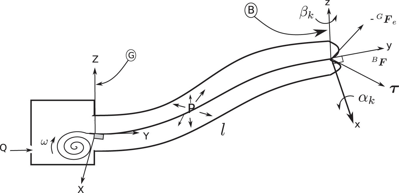
Dynamic model of the vine-growing robot, illustrating forces, actuation inputs, and environmental interactions.
The force
The external forces
The force
where
In practice,
To model the system’s bending response, we incorporate torsion springs at the points of interaction with the environment. This approach can be mathematically expressed as follows:
where
For extended lengths of the vine-growing robot, the weight becomes significant, as it is proportional to the free length
where
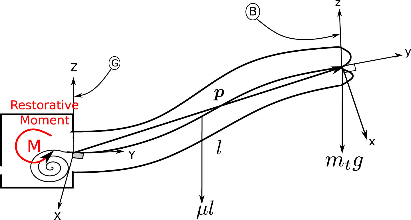
Dynamic force balance of the vine robot. The diagram illustrates the restorative moment
The deflection of the vine robot due to gravitational effects and additional weight is negligible, primarily because the stiffness induced by the internal pressure within the robot’s membrane is significantly greater than the forces caused by these weights. For this assumption to hold, the internal pressure must be sufficiently high to ensure that deflections remain minimal, which justifies the exclusion of these effects in the development of the dynamic equation in (10). Specifically, the principal stress at any point along the backbone of the vine robot must be nonnegative to prevent any significant deformation [34].
To check this posteriori, the axial stress
where
The vine-growing robot can be modeled as a fluid capacitor with a capacitance
where
The fluid capacitance for a given volume of fluid is typically defined as follows:
where
Assuming the vine robot is in thermal equilibrium with the environment and experiences slow changes in pressure and volume, allowing it to maintain a constant temperature, the fluid capacitance of air under isothermal conditions is given by:
where the volume of air
In this context,
When the vine-growing robot is fully extended, the volumetric flow rate into the robot can still be modeled as an ideal capacitor, described by:
where
where
In this context,
Combining equations from (15) to (22), the rate at which the internal pressure
where
These conditions indicate that the robot’s tip cannot extend further and that the tip’s velocity and acceleration are zero once the maximum length is reached.
3.2 The steering model
In contrast to passive environment steering, where the soft growing robot naturally bends around obstacles and follows existing pathways in cluttered and narrow spaces due to its inherent compliance, an active steering mechanism is necessary to control the growth direction for specific tasks. This is especially important in applications that require the creation of deployable and reconfigurable structures. Various steering mechanisms have been developed to control the growth direction of soft growing robots, all based on the principle of altering the relative length of the material on opposite sides of the flexible thin-walled tube. This method induce asymmetric growth by shortening one side to change the robot’s shape and achieve turns, enabling it to curve in space. Recent innovative methods for steering the everting vine robot, which mimic how vine plants explore their surroundings in search of water and nutrients without moving already grown sections, are presented in [11,35].
This study considers a mutually independent, on-demand active steering mechanism as presented in [11]. This steering method uses four pairs of miniature electromagnets and circular plates, which are uniformly distributed at
where
![Figure 5
Schematic diagram of the steering kinematic model [11].](/document/doi/10.1515/nleng-2025-0099/asset/graphic/j_nleng-2025-0099_fig_005.jpg)
Schematic diagram of the steering kinematic model [11].
The rotation angles
The bending angles
This formulation allows for the comprehensive analysis and control of the vine robot’s behavior by incorporating both the growth and steering dynamics within a unified state-space framework.
3.3 Model description
The development of a precise model is crucial for the implementation of model-based control. In this study, we formulate the model using continuous ordinary differential equations and represent it in state-space form. The state vector is defined as
This model effectively captures the complex interplay between the growth and steering mechanisms, enabling precise control of the vine robot’s movements and interactions with its environment.
4 Stress assessment
The internal pressure within the vine robot generates axial stress that propagates along the backbone’s wall to the base. Due to the very small ratio of membrane thickness to diameter, the vine robot primarily experiences circumferential (hoop) stress and longitudinal (axial) stress when pressurized [36]. If the internal pressure causes the stress to exceed the membrane’s maximum capacity, the robot will burst. For simplicity, the tip surface is approximated as a perfect circle with the same diameter as the backbone. The longitudinal stress, assumed to be uniform across the cross-section of the backbone, is given by:
where
Assuming the circumferential stress is uniformly distributed along the length of the vine robot, the circumferential (hoop) stress is expressed as follows:
The circumferential and longitudinal stresses must always be nonnegative and below the yield (burst) stress of the membrane during the robot’s operation.
5 Data-driven dynamic model
In this work, we leverage the power of deep learning techniques due to their flexibility and general representation capabilities to develop a data-driven dynamic model of the everting vine robot using a DNN, as depicted in Figure 6. This DNN serves as a discrete-time dynamic model that can be integrated with model-based controllers. The primary objective of this DNN is to learn the nonlinear mapping from the system state
where
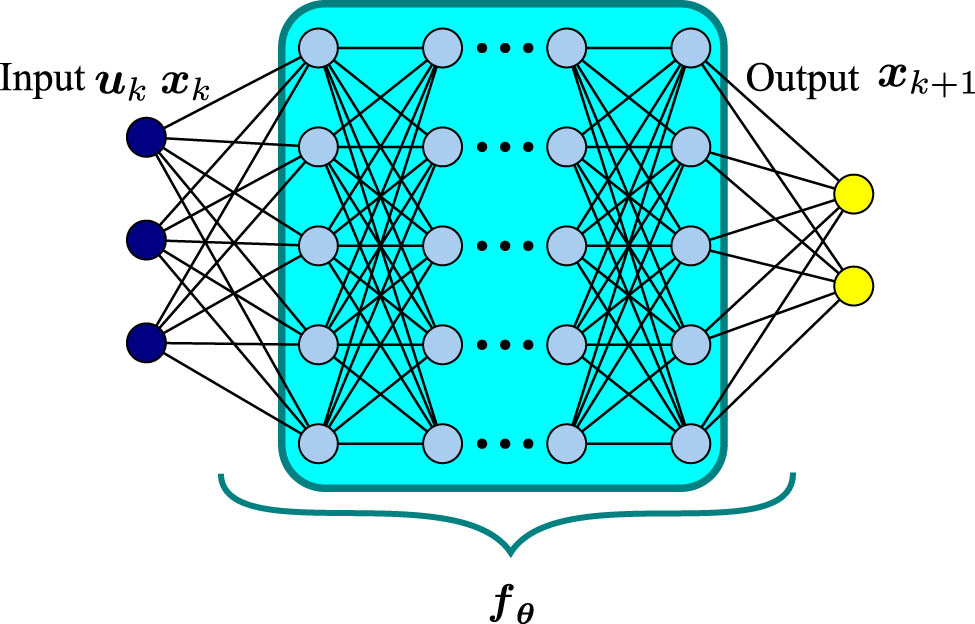
DNN architecture for the everting vine robot.
The DNN employed in this research utilizes fully connected layers with hyperbolic tangent activation functions. It comprises three hidden layers: the first with 32 neurons, the second with 16 neurons, and the third with 8 neurons. The architecture is completed with an output layer that uses a linear activation function to predict the future state
The training data for the DNN are generated from nonlinear simulations of the first-principles model described in Eq. (30). These simulations are conducted using the state-space model with the do-mpc simulator [37] at a sampling time of 0.08 s. The model is driven by sinusoidal forcing functions:
The DNN model is designed and trained using Keras with TensorFlow as the backend engine due to its simple application programming interface and flexibility. After training, normalization layers are incorporated before the input layer and after the output layer to facilitate seamless integration with model-based controllers, ensuring that the input and output data are normalized and denormalized accordingly. Subsequently, the open neural network exchange (ONNX) [38] framework is employed to convert the model from the TensorFlow computation graph to the ONNX format using the tf2onnx package. This conversion enhances interoperability with other Python tools, enabling broader application and integration of the trained model across various platforms.
6 MPC
In this section, we present MPC as a method to simultaneously control the growth and steering of the everting vine robot in free space. MPC, schematically depicted in Figure 7, functions through real-time, iterative optimization using a mathematical surrogate model of the system. The surrogate model employed in this research is a DNN-based discrete-time dynamic model defined in Eq. (33). This approach allows for predicting the future behavior of the robot by solving a potentially constrained optimization problem to determine the optimal trajectory of the manipulated variable

Schematic diagram of model-based predictive control (MPC) for the everting vine robot.
![Figure 8
Illustration of the functional principle of MPC for tracking the reference trajectory, with prediction horizons
N
1
{N}_{1}
and
N
2
{N}_{2}
, and control horizon
N
u
{N}_{u}
(in accordance to the study by Schwenzer et al. [21]). The diagram demonstrates how MPC optimizes and predicts at each time step to ensure the output
y
{\boldsymbol{y}}
follows the desired reference
r
{\boldsymbol{r}}
.](/document/doi/10.1515/nleng-2025-0099/asset/graphic/j_nleng-2025-0099_fig_008.jpg)
Illustration of the functional principle of MPC for tracking the reference trajectory, with prediction horizons
MPC’s widespread adoption in robotics for controlling real systems is attributed to its ability to incorporate constraints directly into the optimization process and its effectiveness in handling nonlinear models, which often exceed the capabilities of classical controllers. This flexibility makes MPC an invaluable tool for achieving precise and reliable control in complex robotic applications.
6.1 Cost function
To achieve precise tracking of the desired reference trajectory while ensuring smooth control behavior, a cost function must be defined to penalize deviations in both the manipulated variable and the trajectory. This cost function is minimized by the optimizer and accounts for deviations from the reference trajectory
s.t.
where
This formulation ensures that the system not only tracks the reference trajectory accurately but also does so with minimal abrupt changes in the control inputs, leading to more stable and efficient operation.
6.2 Constraints and bounds
The system imposes physical constraints and limits on both the actuators and the output
where
6.3 Implementation of MPC
The MPC approach proposed in this study for controlling the vine-growing robot is implemented using the do-mpc framework [37], a Python-based platform for nonlinear and robust MPC. This framework leverages CasADi [39] for symbolic computation and Ipopt [40] for solving nonlinear optimization problems, making it well suited for evaluating the performance and robustness of the proposed controller.
To integrate the DNN-based discrete-time dynamic model of the vine-growing robot, as detailed in Section 5, the model is first converted into a CasADi symbolic expression using the do-mpc ONNXConversion class, which facilitates the conversion from ONNX format. This conversion enables the model to operate as a discrete-time dynamic model within the MPC framework. The nonlinear optimization problem is addressed using Ipopt, which leverages the MA27 linear solver, while the dynamic model’s simulation is carried out using the cvodes tool. This approach ensures precise simulation and optimization, thereby supporting the robust real-time control of the vine-growing robot.
7 Results and discussion
To evaluate the effectiveness of the DNN-based discrete-time dynamic model of the vine-growing robot and assess the performance of the nonlinear robust MPC, simulations are conducted in two distinct settings: open-loop prediction and closed-loop control.
First, an open-loop prediction is performed using the proposed DNN model to compare the predicted system states with those obtained from the nonlinear first-principles model. This comparison allows us to assess the accuracy of the DNN in estimating the system’s dynamics.
Second, to evaluate the effectiveness and performance of the proposed MPC in controlling both the growth and steering of the vine-growing robot, a closed-loop simulation is conducted. This simulation ensures that the system states achieve the desired setpoints or follow the specified trajectory under the control of the MPC. The closed-loop simulations are executed using the do-mpc framework.
The parameters used for simulating the vine-growing robot are presented in Table 1. Notably, the magnitude of the fictitious mass
Simulation parameters for vine-growing robot
| Parameter | Description | Value |
|---|---|---|
|
|
Fictitious mass |
|
|
|
Fully extended length of the robot | 1.2 m |
|
|
Atmospheric pressure | 101325 Pa |
|
|
Yield pressure |
|
|
|
Radius of the spool | 0.025 m |
|
|
Diameter of the membrane | 0.0798 m |
|
|
Thickness of the membrane | 0.0001 m |
|
|
Thickness of the electromagnet unit | 0.012 m |
|
|
Torsional stiffness | 22 Nm/rad |
|
|
Weight per unit length | 0.008 N/m |
|
|
Stiffness of the membrane |
|
|
|
Cross-sectional area of the tip |
|
|
|
Gravitational acceleration constant | 9.81 m/s2 |
|
|
Radius of the membrane | 0.0399 m |
7.1 Performance of the DNN dynamic model of the vine robot
In this section, we evaluate the performance of the DNN-based discrete-time dynamic model for the pressure-driven everting vine robot, which is intended for integration into the MPC as a surrogate model. The DNN model is trained using Keras with TensorFlow as the backend engine, running on an Intel Core i5-4300M CPU @ 2.60 GHz with 7.4 GB of RAM. This setup allows us to assess the model’s accuracy and computational efficiency, ensuring it is suitable for real-time control applications within the MPC framework.
To evaluate the performance of the proposed DNN-based dynamic model for the vine robot, the training and validation loss were monitored over 200 epochs on normalized data. The Adam optimizer was employed with a learning rate of 0.001. Figure 9 illustrates the training and validation loss curves, both of which show the mean squared error (MSE) steadily converging. The rapid decrease in MSE during the initial epochs indicates effective learning, and the subsequent stabilization suggests that the model is not overfitting, maintaining consistent performance across both training and validation datasets.
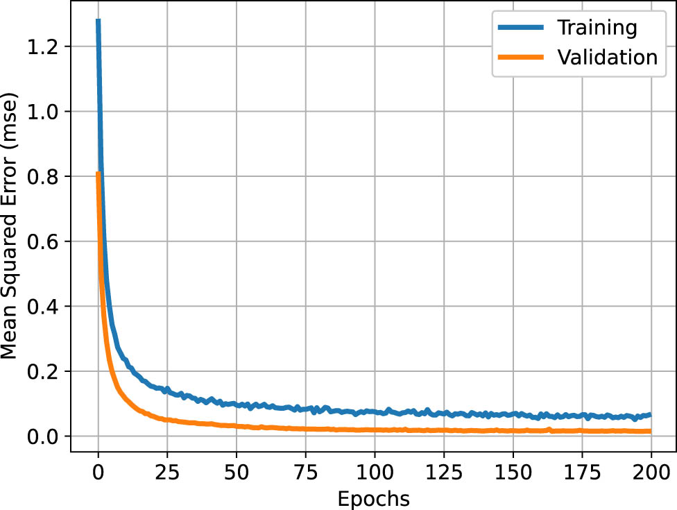
Training performance of the DNN model.
Figure 10 illustrates the open-loop predictions of the system states using the DNN-based model, compared to the actual states derived from the first-principles model. The comparison shows that the differences between the DNN-predicted states and the first-principles model’s states are minimal, indicating a high level of accuracy in the DNN model’s predictions. This close alignment validates the use of the proposed DNN model as an effective surrogate for the more complex first-principles model, demonstrating its potential for integration into the MPC framework.
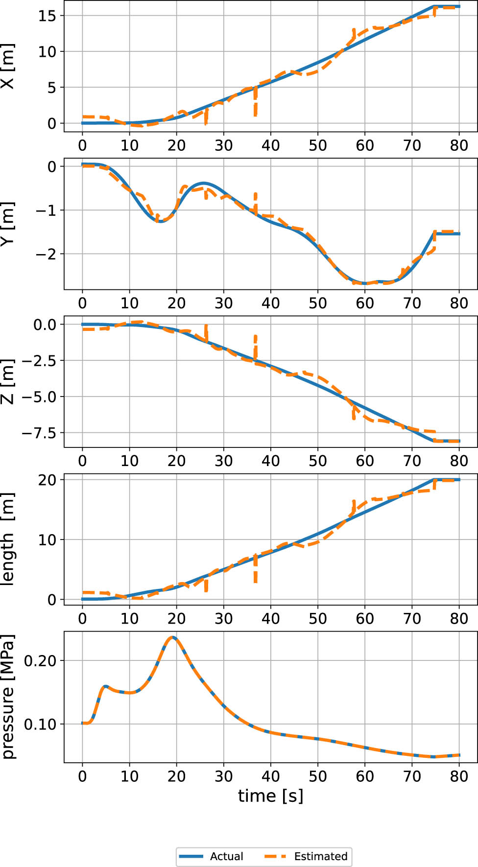
Comparison of the time evolution of system states between the nonlinear first-principles model and the DNN-predicted model.
To assess the generalization performance of the proposed DNN for the pressure-driven everting vine robot, a K-fold cross-validation approach was employed, as recommended by Marcot and Hanea [42]. This method is vital for identifying a robust architecture that exhibits minimal sensitivity to variations in training data partitions. In this study, the dataset was divided into five folds, and five distinct feed-forward DNN models were evaluated for performance. These models, varying in complexity, each comprise fully connected hidden layers as detailed in Table 2. The layers are denoted by “F” with subscripts indicating the number of neurons in each layer. All hidden layers utilize hyperbolic tangent activation functions, while the output layer employs a linear activation function. This systematic evaluation ensures the selection of a DNN architecture that balances complexity and performance, optimizing the model’s ability to generalize to unseen data.
Comparison of models with different hidden layer configurations and their corresponding average MSE with standard deviation
| Model | hidden layers | Avg. MSE (
|
|---|---|---|
| 1 | F128, F32, F16 | 7.78
|
| 2 | F256, F128, F32 | 5.14
|
| 3 | F512, F256, F32 | 4.99
|
| 4 | F512, F512, F128, F64 | 4.31
|
| 5 | F512, F512, F128, F64 | 3.68
|
The models were trained for 100 epochs using the Adam optimizer, with MSE as the primary loss metric. The convergence of the learning curves during five-fold cross-validation for all network configurations is depicted in Figure 11. The learning curves demonstrate that models with higher complexity, indicated by darker shades of red, tend to converge faster and stabilize more effectively, reflecting the models’ capacity to capture the underlying dynamics of the system more accurately.
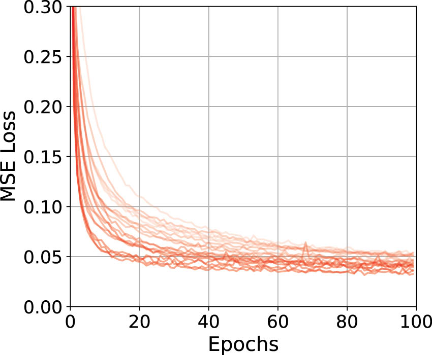
Training losses for five DNN models during five-fold cross-validation.
In addition, Figure 12 illustrates the average mean squared error and their standard deviations across different model architectures. The results show a clear trend where increased model complexity leads to lower MSE values, indicating improved predictive performance. However, this comes with the trade-off of increased computational cost and potential overfitting, as evidenced by the greater variability in some of the more complex models. These findings highlight the critical need to balance model complexity and generalization capability when selecting the optimal architecture for the vine robot’s dynamic model, ensuring both accuracy and robustness in real-world applications.
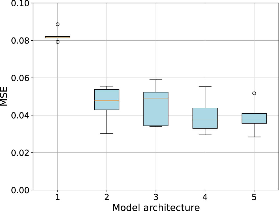
Average MSE and standard deviation.
7.2 Closed-loop simulation
To evaluate the performance and capabilities of integrating the DNN-based discrete-time dynamic model with the MPC framework, we conducted a comparative analysis between the DNN dynamic model and the first-principles model across three tracking control scenarios: set-point stabilization, obstacle avoidance, and trajectory tracking. The MPC was designed using both the first-principles model and the DNN model, allowing us to assess the performance improvements offered by a data-driven approach in controlling a nonlinear dynamic system in real-time applications. This comparison highlights the potential advantages of utilizing DNN-based models for enhanced accuracy and efficiency in complex control tasks.
7.2.1 Set-point stabilization
The performance of the proposed MPC, utilizing both DNN-based and first-principles dynamic models, is evaluated based on its ability to precisely track a desired setpoint in space. This capability is particularly vital for applications such as medical procedures, where the vine robot may be required to deliver drugs accurately to a specific organ from its base. In this study, the control objective is to guide the robot to a specific position in Cartesian space, ensuring that it comes to rest with the desired force. The target state is set as
The weighting matrices used in the MPC formulation are
In addition to the system constraints outlined in Section 6, the robot’s position is further constrained within the following bounds:
These constraints ensure that the robot operates within a safe and feasible region while achieving the control objectives. This scenario highlights the effectiveness of the proposed MPC in maintaining precise control of the vine robot under the specified conditions.
The dynamic model is initialized with initial state of
Figure 13 compares the performance of the DNN-based dynamic model with the first-principles model during closed-loop control, illustrating the evolution of system states, stresses, and actuation inputs over time.
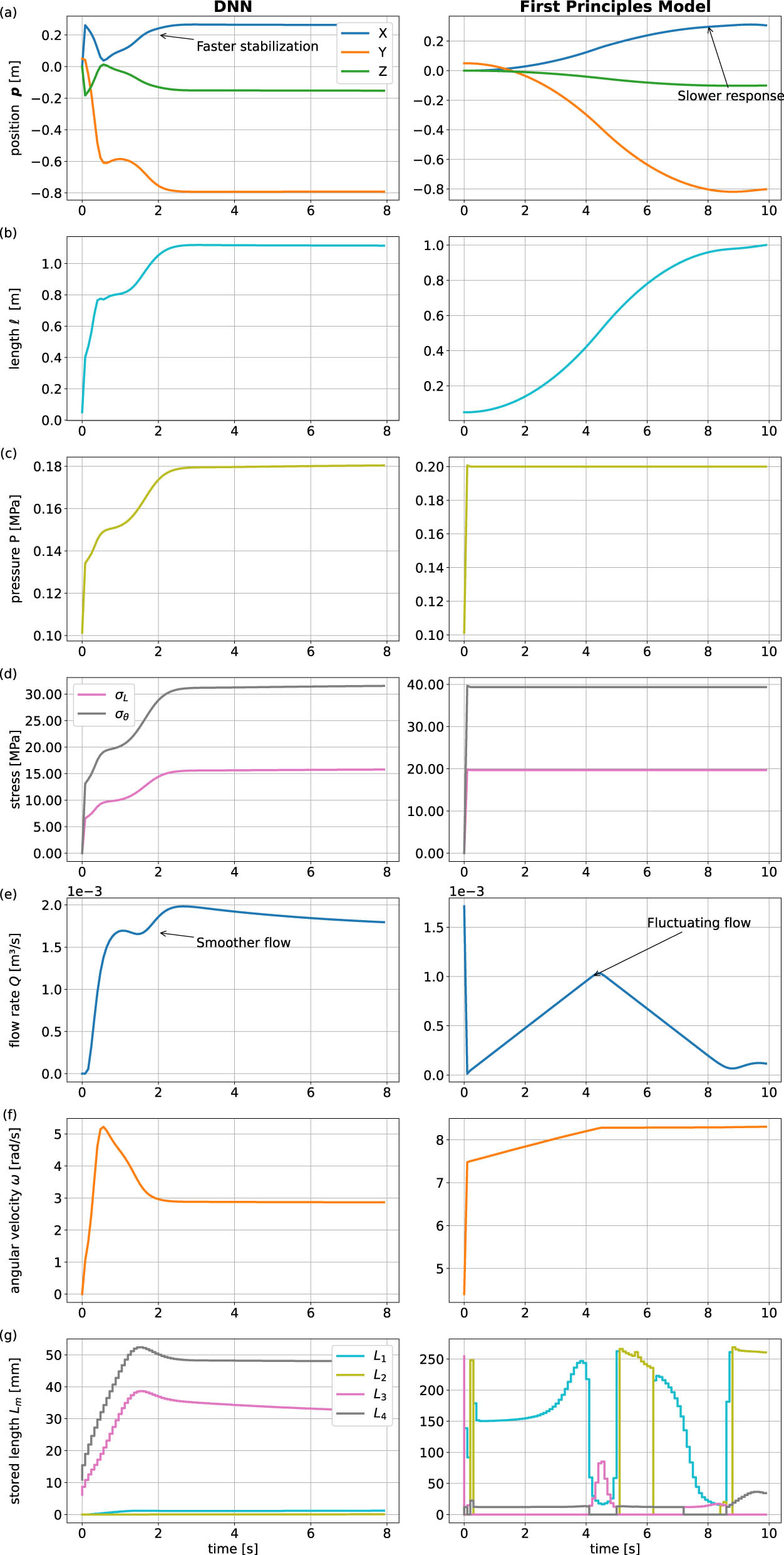
Comparison of the closed-loop control performance of the DNN-based dynamic model and the first-principles model for set-point stabilization simulation. (a) Position tracking
In this comparison, both the DNN-based model and the first-principles model achieve effective set-point stabilization, with the DNN model showing slightly faster convergence in the position states (
The results indicate that the average time taken by the MPC solver to find the optimal control with the DNN dynamic model is 2.2 times faster than using the first-principles model. This improvement in computational efficiency is particularly useful in real-time applications, where the prediction horizon can be five times shorter compared to that of the analytical model.
Overall, these figures highlight the advantages of the DNN-based model in achieving quicker and more stable control responses while requiring less aggressive actuation. This suggests that the DNN model can offer superior performance in real-time control scenarios, providing a viable alternative to more computationally intensive first-principles models.
7.2.2 Obstacle avoidance
In this section, the effectiveness of the proposed MPC is evaluated in the context of obstacle avoidance, a crucial capability for navigating cluttered environments such as archaeological excavation sites. The obstacle is positioned at
To ensure the robot successfully avoids the obstacle, a nonlinear inequality constraint is introduced into the optimization problem. This constraint enforces that the Euclidean distance between the tip of the vine robot and the center of the obstacle remains above a specified safety threshold:
where
The simulation results using both the DNN-based discrete-time dynamic model and the first-principles model, depicted in Figure 14, demonstrate that the proposed MPC successfully navigated the vine robot around the obstacle and achieved the desired setpoint. The corresponding actuation inputs and system states during the obstacle avoidance maneuver are shown in Figure 15.
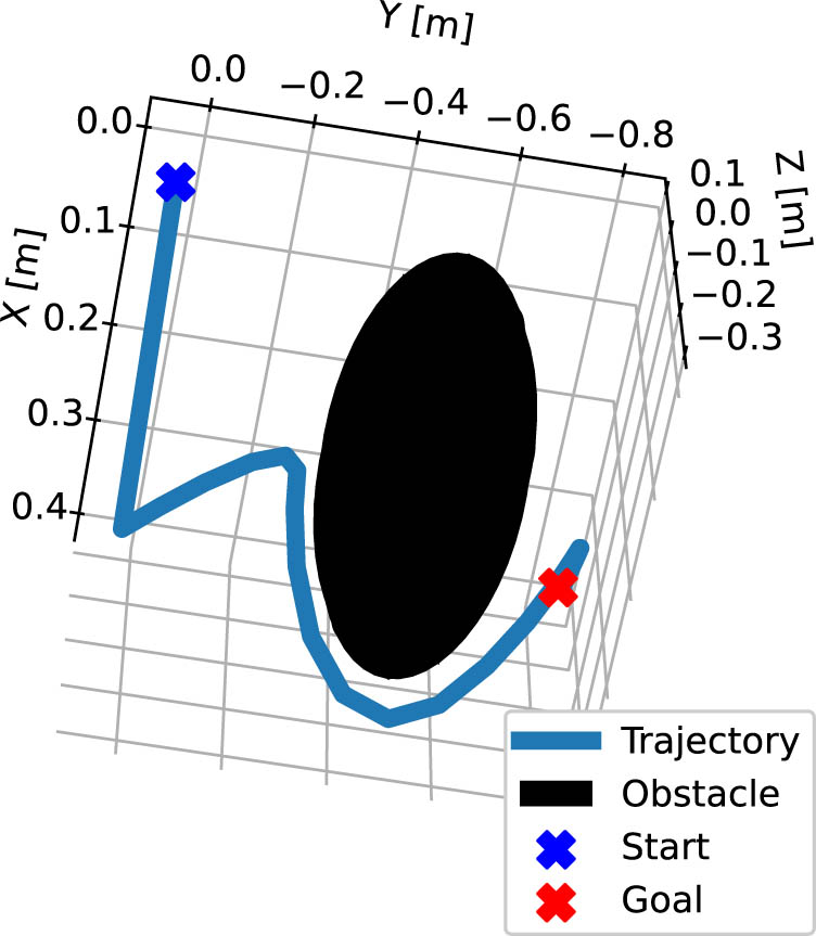
Simulation results of vine robot avoiding an obstacle in Cartesian space.
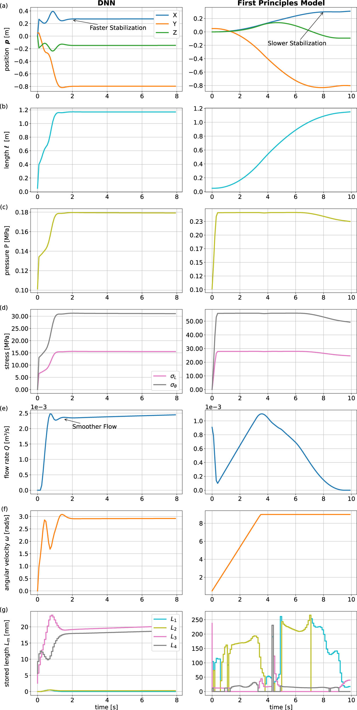
Closed-loop control performance comparison between the DNN-based dynamic model and the first-principles model during obstacle avoidance. (a) Position
The results confirm that the proposed MPC effectively guides the vine robot in avoiding the obstacle while maintaining the desired trajectory. Notably, the DNN-MPC architecture significantly outperformed the MPC framework based on the first-principles model in terms of computation time, with the DNN-MPC being 7.2 times faster than its counterpart. This substantial improvement in computational efficiency highlights the DNN-based approach’s potential for real-time applications, where quick decision-making is crucial for effective obstacle avoidance and trajectory control.
7.2.3 Trajectory tracking
In this final evaluation, a time-varying trajectory from the dataset is used to assess the effectiveness of the proposed MPC in tracking dynamic paths with the surrogate models. This scenario is particularly relevant for applications requiring a soft, reconfigurable, and deployable antenna, such as those that need to assume various shapes like a helix. The ability to accurately follow such trajectories is crucial for ensuring the antenna’s functionality in diverse operational environments.
All tuning parameters for the MPC, including the prediction horizon, weighting matrices, and constraints, are consistent with those presented in Section 7.2.1. This consistency allows for a direct comparison of the controller’s performance in both set-point stabilization and more complex trajectory tracking tasks, demonstrating the robustness and versatility of the proposed MPC framework.
Figure 16 illustrates the motion of the vine robot in space while tracking a time-varying trajectory. The performance of the proposed MPC, utilizing both the DNN-based dynamic model and the first-principles model, is presented in Figure 17, along with the corresponding actuation inputs to the system. The results show that the DNN-MPC architecture tracks the trajectory more effectively, achieving faster convergence and more precise alignment with the reference trajectory compared to the first-principles model. Furthermore, the DNN-MPC architecture demonstrates smoother and more efficient actuation, resulting in better overall control performance compared to the first-principles model.
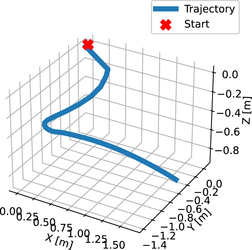
3D motion of the vine robot while tracking a time-varying trajectory.
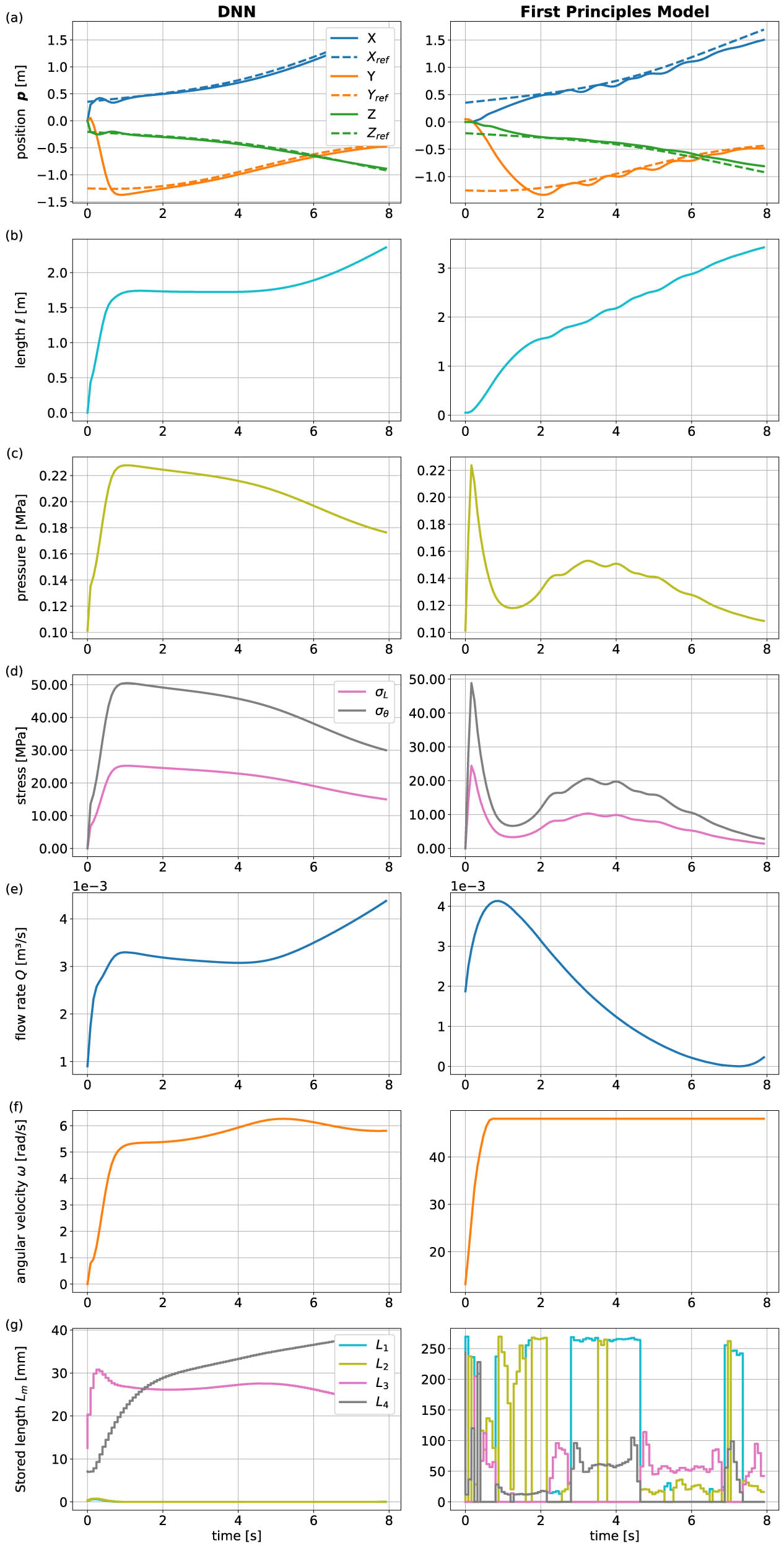
Closed-loop control performance comparison between the DNN-based dynamic model and the first-principles model during for the trajectory tracking task of the vine growing robot. (a) Position
Significantly, the DNN-MPC architecture outperformed the first-principles model-based MPC framework in terms of computation time, with the DNN-MPC being 11 times faster. This substantial improvement highlights the DNN model’s suitability for real-time control applications, where computational efficiency is critical for responsive and accurate trajectory tracking.
8 Conclusions
This study proposed a data-driven dynamic model of a pressure-driven everting vine robot using a DNN architecture as a discrete-time dynamic model to control its growth and direction. The DNN model was trained using data generated by the nonlinear simulation of the first-principles model of the everting vine robot. A K-fold cross-validation approach was employed to assess the general performance of the proposed DNN model for the vine robot, which subsequently informed the selection of the optimal architecture based on average MSE. The data-driven model was then integrated into a MPC framework to evaluate its computational tractability and effectiveness in controlling the nonlinear dynamics of the vine robot.
The comparative analysis between the DNN-MPC and the traditional MPC based on the nonlinear first-principles model revealed that the DNN-MPC framework provided superior control performance while significantly reducing computation time. This indicates that the DNN-MPC framework is a promising approach for efficient and effective data-driven nonlinear control of soft robotic systems.
This work opens up several avenues for future research and exploration. Although this study assumed full state measurement, in practice, some states may be difficult to measure directly. In such cases, state estimators like moving horizon estimator can be employed to estimate unmeasured states from the available measurements. In addition, other data-driven discovery techniques, such as sparse identification of nonlinear dynamics (SINDy), could be explored to develop more parsimonious and interpretable models, offering greater insights compared to DNN models, which are often considered black boxes and do not easily incorporate known constraints.
Furthermore, DNN models typically require large quantities of significant data to train effectively, especially when dealing with the complex and nonlinear dynamics of soft robots. This can be challenging to obtain and may limit the model’s ability to generalize beyond the training data. To address this, physics-informed neural networks (PINNs), which embed known physical laws governing the system into the NNs, could be utilized. PINNs require less training data compared to traditional NNs, thus providing a more robust DNN model that converges faster and generalizes well to unseen data.
In applications involving human–robot interactions, such as minimally invasive surgery, it is not sufficient to control only the position and velocity of the vine robot. Equally important is regulating how the robot responds to forces exerted by its environment. To address this, an impedance controller based on a DNN-discrete model is essential for regulating the interaction between the robot’s tip and the human body, where compliance and safety are critical. Such approaches have the potential to significantly enhance the performance, adaptability, and applicability of DNN-based control systems across a wide range of soft robotic applications.
Acknowledgments
This research was supported by EJUST-TICAD8 scholarship through JICA and the government of Japan and Egypt for the first author.
-
Funding information: The authors state no funding involved.
-
Author contributions: All authors have accepted responsibility for the entire content of this manuscript and consented to its submission to the journal, reviewed all the results, and approved the final version of the manuscript.
-
Conflict of interest: The authors state no conflict of interest.
-
Data availability statement: All data that support the findings of this study are included within the article.
References
[1] Meder F, Baytekin B, Del Dottore E, Meroz Y, Tauber F, Walker I, et al. A perspective on plant robotics: from bioinspiration to hybrid systems. Bioinspirat Biomimetics. 2023 Jan;18(1):015006. 10.1088/1748-3190/aca198Suche in Google Scholar PubMed
[2] Gährs C, Vidal-Gadea A. Locomotion. In: Encyclopedia of animal cognition and behavior. Cham: Springer International Publishing; 2022. p. 3986–4001. 10.1007/978-3-319-55065-7_1450Suche in Google Scholar
[3] Mano H, Hasebe M. Rapid movements in plants. J Plant Res. 2021 Jan;134(1):3–17. 10.1007/s10265-020-01243-7Suche in Google Scholar PubMed PubMed Central
[4] Fiorello I, Del Dottore E, Tramacere F, Mazzolai B. Taking inspiration from climbing plants: methodologies and benchmarks-a review. Bioinspirat Biomimetics. 2020 May;15(3):031001. 10.1088/1748-3190/ab7416Suche in Google Scholar PubMed
[5] Dent EW, Gertler FB. Cytoskeletal dynamics and transport in growth cone motility and axon guidance. Neuron. 2003 Oct;40(2):209–27. 10.1016/S0896-6273(03)00633-0Suche in Google Scholar PubMed
[6] Palanivelu R, Preuss D. Pollen tube targeting and axon guidance: parallels in tip growth mechanisms. Trends Cell Biol. 2000 Dec;10(12):517–24. 10.1016/S0962-8924(00)01849-3Suche in Google Scholar
[7] Vidoni R, Mimmo T, Pandolfi C. Tendril-based climbing plants to model, simulate and create bio-inspired robotic systems. J Bionic Eng. 2015 June;12(2):250–62. 10.1016/S1672-6529(14)60117-7Suche in Google Scholar
[8] Mazzolai B, Tramacere F, Fiorello I, Margheri L. The bio-engineering approach for plant investigations and growing robots. A Mini-Review. Front Robotics AI. 2020 Sep;7:573014. 10.3389/frobt.2020.573014Suche in Google Scholar PubMed PubMed Central
[9] Blumenschein LH, Coad MM, Haggerty DA, Okamura AM, Hawkes EW. Design, modeling, control, and application of everting vine robots. Front Robot AI. 2020 Nov;7(November):1–24. 10.3389/frobt.2020.548266Suche in Google Scholar PubMed PubMed Central
[10] Haggerty DA, Naclerio ND, Hawkes EW. Characterizing environmental interactions for soft growing robots. In: 2019 IEEE/RSJ International Conference on Intelligent Robots and Systems (IROS). IEEE; 2019. p. 3335–42. 10.1109/IROS40897.2019.8968137Suche in Google Scholar
[11] Li P, Zhang Y, Zhang G, Zhou D, Li L. A bioinspired soft robot combining the growth adaptability of vine plants with a coordinated control system. Research. 2021 Jan;2021:9843859. 10.34133/2021/9843859Suche in Google Scholar PubMed PubMed Central
[12] Hawkes EW, Blumenschein LH, Greer JD, Okamura AM. A soft robot that navigates its environment through growth. Sci Robot. 2017 Jul;2(8):1–8. 10.1126/scirobotics.aan3028Suche in Google Scholar PubMed
[13] Naclerio ND, Hubicki CM, Aydin YO, Goldman DI, Hawkes EW. Soft robotic burrowing device with tip-extension and granular fluidization. In: 2018 IEEE/RSJ International Conference on Intelligent Robots and Systems (IROS). IEEE; 2018. p. 5918–23. 10.1109/IROS.2018.8593530Suche in Google Scholar
[14] Putzu F, Abrar T, Althoefer K. Plant-inspired soft pneumatic eversion robot. In: 2018 7th IEEE International Conference on Biomedical Robotics and Biomechatronics (Biorob). vol. 2018-Augus. IEEE; 2018. p. 1327–32. 10.1109/BIOROB.2018.8487848Suche in Google Scholar
[15] Blumenschein LH, Gan LT, Fan JA, Okamura AM, Hawkes EW. A tip-extending soft robot enables reconfigurable and deployable antennas. IEEE Robot Automat Lett. 2018 Apr;3(2):949–56. 10.1109/LRA.2018.2793303Suche in Google Scholar
[16] Webster RJ, Jones BA. Design and kinematic modeling of constant curvature continuum robots: a review. Int J Robot Res. 2010 Nov;29(13):1661–83. 10.1177/0278364910368147Suche in Google Scholar
[17] Gravagne IA, Rahn CD, Walker ID. Large deflection dynamics and control for planar continuum robots. IEEE/ASME Trans Mechatronics. 2003 June;8(2):299–307. 10.1109/TMECH.2003.812829Suche in Google Scholar
[18] El-Hussieny H, Hameed IA, Ryu JH. Nonlinear model predictive growth control of a class of plant-inspired soft growing robots. IEEE Access. 2020;8:214495–503. 10.1109/ACCESS.2020.3041616Suche in Google Scholar
[19] Wu Z, Reyzabal MDI, Sadati SMH, Liu H, Ourselin S, Leff D, et al. Towards a physics-based model for steerable eversion growing robots. IEEE Robot Automat Letters. 2023 Feb;8(2):1005–12. 10.1109/LRA.2023.3234823Suche in Google Scholar PubMed PubMed Central
[20] Talas SK, Baydere BA, Altinsoy T, Tutcu C, Samur E. Design and development of a growing pneumatic soft robot. Soft Robotics. 2020 Aug;7(4):521–33. 10.1089/soro.2019.0083Suche in Google Scholar PubMed
[21] Schwenzer M, Ay M, Bergs T, Abel D. Review on model predictive control: an engineering perspective. Int J Adv Manufact Tech. 2021 Nov;117(5-6):1327–49. 10.1007/s00170-021-07682-3Suche in Google Scholar
[22] Kaiser E, Kutz JN, Brunton SL. Sparse identification of nonlinear dynamics for model predictive control in the low-data limit. Proc R Soc A Math Phys Eng Sci. 2018 Nov;474(2219):20180335. 10.1098/rspa.2018.0335Suche in Google Scholar PubMed PubMed Central
[23] Blumenschein LH, Okamura AM, Hawkes EW. Modeling of bioinspired apical extension in a soft robot. vol. 1; 2017. p. 522–31. 10.1007/978-3-319-63537-8_45Suche in Google Scholar
[24] Tutcu C, Baydere BA, Talas SK, Samur E. Quasi-static modeling of a novel growing soft-continuum robot. Int J Robot Res. 2021 Jan;40(1):86–98. 10.1177/0278364919893438Suche in Google Scholar
[25] Jitosho R, Agharese N, Okamura A, Manchester Z. A dynamics simulator for soft growing robots. Proceedings - IEEE International Conference on Robotics and Automation. 2021;2021-May(Icra):11775–11781. 10.1109/ICRA48506.2021.9561420Suche in Google Scholar
[26] Lusch B, Kutz JN, Brunton SL. Deep learning for universal linear embeddings of nonlinear dynamics. Nature Commun. 2018 Nov;9(1):4950. 10.1038/s41467-018-07210-0Suche in Google Scholar PubMed PubMed Central
[27] Sapai S, Loo JY, Ding ZY, Tan CP, Baskaran VM, Nurzaman SG. A deep learning framework for soft robots with synthetic data. Soft Robot. 2023 Dec;10(6):1224–40. 10.1089/soro.2022.0188Suche in Google Scholar PubMed
[28] Cespedes A, Terreros R, Morales S, Huamani A, Canahuire R. Dynamic modeling of a soft laparoscope: A deep neural network approach. In: 2022 Latin American Robotics Symposium (LARS), 2022 Brazilian Symposium on Robotics (SBR), and 2022 Workshop on Robotics in Education (WRE). IEEE; 2022. p. 1–6. 10.1109/LARS/SBR/WRE56824.2022.9995831Suche in Google Scholar
[29] Hyatt P, Wingate D, Killpack MD. Model-based control of soft actuators using learned non-linear discrete-time models. Front Robot AI. 2019 Apr;6(APR):1–11. 10.3389/frobt.2019.00022Suche in Google Scholar PubMed PubMed Central
[30] Greer JD, Morimoto TK, Okamura AM, Hawkes EW. A soft, steerable continuum robot that grows via tip extension. Soft Robot. 2019 Feb;6(1):95–108. 10.1089/soro.2018.0034Suche in Google Scholar PubMed
[31] Neppalli S, Jones BA. Design, construction, and analysis of a continuum robot. In: 2007 IEEE/RSJ International Conference on Intelligent Robots and Systems. IEEE; 2007. p. 1503–7. 10.1109/IROS.2007.4399275Suche in Google Scholar
[32] Gan LT, Blumenschein LH, Huang Z, Okamura AM, Hawkes EW, Fan JA. 3D electromagnetic reconfiguration enabled by soft continuum robots. IEEE Robot Automat Lett. 2020 Apr;5(2):1704–11. 10.1109/LRA.2020.2969922Suche in Google Scholar
[33] Coad MM, Blumenschein LH, Cutler S, Zepeda JAR, Naclerio ND, El-Hussieny H, et al. Vine robots. IEEE Robot Automat Magazine. 2020 Sep;27(3):120–32. 10.1109/MRA.2019.2947538Suche in Google Scholar
[34] Levan A, Wielgosz C. Bending and buckling of inflatable beams: Some new theoretical results. Thin-Walled Struct. 2005 Aug;43(8):1166–87. 10.1016/j.tws.2005.03.005Suche in Google Scholar
[35] Bianchi G, Agoni A, Cinquemani S. A bioinspired robot growing like plant roots. J Bionic Eng. 2023;20(5):2044–58. 10.1007/s42235-023-00369-3Suche in Google Scholar
[36] Godaba H, Putzu F, Abrar T, Konstantinova J, Althoefer K. Payload capabilities and operational limits of eversion robots. In: Lecture Notes in Computer Science (including subseries Lecture Notes in Artificial Intelligence and Lecture Notes in Bioinformatics). vol. 11650 LNAI. Springer International Publishing; 2019. p. 383–94. 10.1007/978-3-030-25332-5_33Suche in Google Scholar
[37] Fiedler F, Karg B, Lüken L, Brandner D, Heinlein M, Brabender F, et al. do-mpc: Towards FAIR nonlinear and robust model predictive control. Control Eng Practice. 2023 Nov;140(September):105676. 10.1016/j.conengprac.2023.105676Suche in Google Scholar
[38] ONNX. Open Neural Network Exchange (ONNX); 2020. Suche in Google Scholar
[39] Andersson JAE, Gillis J, Horn G, Rawlings JB, Diehl M. CasADi: a software framework for nonlinear optimization and optimal control. Math Program Comput. 2019 Mar;11(1):1–36. 10.1007/s12532-018-0139-4Suche in Google Scholar
[40] Wächter A, Biegler LT. On the implementation of an interior-point filter line-search algorithm for large-scale nonlinear programming. Math Program. 2006 Mar;106(1):25–57. 10.1007/s10107-004-0559-ySuche in Google Scholar
[41] Kalibala A, Nada AA, Ishii H, El-Hussieny H. Dynamic modelling and predictive position/force control of a plant-inspired growing robot. Bioinspirat Biomimetics. 2025 Jan;20:016005. 10.1088/1748-3190/ad8e25Suche in Google Scholar PubMed
[42] Marcot BG, Hanea AM. What is an optimal value of k in k-fold cross-validation in discrete Bayesian network analysis? Comput Stat. 2021 Sep;36(3):2009–31. 10.1007/s00180-020-00999-9Suche in Google Scholar
© 2025 the author(s), published by De Gruyter
This work is licensed under the Creative Commons Attribution 4.0 International License.
Artikel in diesem Heft
- Research Articles
- Generalized (ψ,φ)-contraction to investigate Volterra integral inclusions and fractal fractional PDEs in super-metric space with numerical experiments
- Solitons in ultrasound imaging: Exploring applications and enhancements via the Westervelt equation
- Stochastic improved Simpson for solving nonlinear fractional-order systems using product integration rules
- Exploring dynamical features like bifurcation assessment, sensitivity visualization, and solitary wave solutions of the integrable Akbota equation
- Research on surface defect detection method and optimization of paper-plastic composite bag based on improved combined segmentation algorithm
- Impact the sulphur content in Iraqi crude oil on the mechanical properties and corrosion behaviour of carbon steel in various types of API 5L pipelines and ASTM 106 grade B
- Unravelling quiescent optical solitons: An exploration of the complex Ginzburg–Landau equation with nonlinear chromatic dispersion and self-phase modulation
- Perturbation-iteration approach for fractional-order logistic differential equations
- Variational formulations for the Euler and Navier–Stokes systems in fluid mechanics and related models
- Rotor response to unbalanced load and system performance considering variable bearing profile
- DeepFowl: Disease prediction from chicken excreta images using deep learning
- Channel flow of Ellis fluid due to cilia motion
- A case study of fractional-order varicella virus model to nonlinear dynamics strategy for control and prevalence
- Multi-point estimation weldment recognition and estimation of pose with data-driven robotics design
- Analysis of Hall current and nonuniform heating effects on magneto-convection between vertically aligned plates under the influence of electric and magnetic fields
- A comparative study on residual power series method and differential transform method through the time-fractional telegraph equation
- Insights from the nonlinear Schrödinger–Hirota equation with chromatic dispersion: Dynamics in fiber–optic communication
- Mathematical analysis of Jeffrey ferrofluid on stretching surface with the Darcy–Forchheimer model
- Exploring the interaction between lump, stripe and double-stripe, and periodic wave solutions of the Konopelchenko–Dubrovsky–Kaup–Kupershmidt system
- Computational investigation of tuberculosis and HIV/AIDS co-infection in fuzzy environment
- Signature verification by geometry and image processing
- Theoretical and numerical approach for quantifying sensitivity to system parameters of nonlinear systems
- Chaotic behaviors, stability, and solitary wave propagations of M-fractional LWE equation in magneto-electro-elastic circular rod
- Dynamic analysis and optimization of syphilis spread: Simulations, integrating treatment and public health interventions
- Visco-thermoelastic rectangular plate under uniform loading: A study of deflection
- Threshold dynamics and optimal control of an epidemiological smoking model
- Numerical computational model for an unsteady hybrid nanofluid flow in a porous medium past an MHD rotating sheet
- Regression prediction model of fabric brightness based on light and shadow reconstruction of layered images
- Dynamics and prevention of gemini virus infection in red chili crops studied with generalized fractional operator: Analysis and modeling
- Qualitative analysis on existence and stability of nonlinear fractional dynamic equations on time scales
- Fractional-order super-twisting sliding mode active disturbance rejection control for electro-hydraulic position servo systems
- Analytical exploration and parametric insights into optical solitons in magneto-optic waveguides: Advances in nonlinear dynamics for applied sciences
- Bifurcation dynamics and optical soliton structures in the nonlinear Schrödinger–Bopp–Podolsky system
- User profiling in university libraries by combining multi-perspective clustering algorithm and reader behavior analysis
- Review Article
- Haar wavelet collocation method for existence and numerical solutions of fourth-order integro-differential equations with bounded coefficients
- Special Issue: Nonlinear Analysis and Design of Communication Networks for IoT Applications - Part II
- Silicon-based all-optical wavelength converter for on-chip optical interconnection
- Research on a path-tracking control system of unmanned rollers based on an optimization algorithm and real-time feedback
- Analysis of the sports action recognition model based on the LSTM recurrent neural network
- Industrial robot trajectory error compensation based on enhanced transfer convolutional neural networks
- Research on IoT network performance prediction model of power grid warehouse based on nonlinear GA-BP neural network
- Interactive recommendation of social network communication between cities based on GNN and user preferences
- Application of improved P-BEM in time varying channel prediction in 5G high-speed mobile communication system
- Construction of a BIM smart building collaborative design model combining the Internet of Things
- Optimizing malicious website prediction: An advanced XGBoost-based machine learning model
- Economic operation analysis of the power grid combining communication network and distributed optimization algorithm
- Sports video temporal action detection technology based on an improved MSST algorithm
- Internet of things data security and privacy protection based on improved federated learning
- Enterprise power emission reduction technology based on the LSTM–SVM model
- Construction of multi-style face models based on artistic image generation algorithms
- Research and application of interactive digital twin monitoring system for photovoltaic power station based on global perception
- Special Issue: Decision and Control in Nonlinear Systems - Part II
- Animation video frame prediction based on ConvGRU fine-grained synthesis flow
- Application of GGNN inference propagation model for martial art intensity evaluation
- Benefit evaluation of building energy-saving renovation projects based on BWM weighting method
- Deep neural network application in real-time economic dispatch and frequency control of microgrids
- Real-time force/position control of soft growing robots: A data-driven model predictive approach
- Mechanical product design and manufacturing system based on CNN and server optimization algorithm
- Application of finite element analysis in the formal analysis of ancient architectural plaque section
- Research on territorial spatial planning based on data mining and geographic information visualization
- Fault diagnosis of agricultural sprinkler irrigation machinery equipment based on machine vision
- Closure technology of large span steel truss arch bridge with temporarily fixed edge supports
- Intelligent accounting question-answering robot based on a large language model and knowledge graph
- Analysis of manufacturing and retailer blockchain decision based on resource recyclability
- Flexible manufacturing workshop mechanical processing and product scheduling algorithm based on MES
- Exploration of indoor environment perception and design model based on virtual reality technology
- Tennis automatic ball-picking robot based on image object detection and positioning technology
- A new CNN deep learning model for computer-intelligent color matching
- Design of AR-based general computer technology experiment demonstration platform
- Indoor environment monitoring method based on the fusion of audio recognition and video patrol features
- Health condition prediction method of the computer numerical control machine tool parts by ensembling digital twins and improved LSTM networks
- Establishment of a green degree evaluation model for wall materials based on lifecycle
- Quantitative evaluation of college music teaching pronunciation based on nonlinear feature extraction
- Multi-index nonlinear robust virtual synchronous generator control method for microgrid inverters
- Manufacturing engineering production line scheduling management technology integrating availability constraints and heuristic rules
- Analysis of digital intelligent financial audit system based on improved BiLSTM neural network
- Attention community discovery model applied to complex network information analysis
- A neural collaborative filtering recommendation algorithm based on attention mechanism and contrastive learning
- Rehabilitation training method for motor dysfunction based on video stream matching
- Research on façade design for cold-region buildings based on artificial neural networks and parametric modeling techniques
- Intelligent implementation of muscle strain identification algorithm in Mi health exercise induced waist muscle strain
- Optimization design of urban rainwater and flood drainage system based on SWMM
- Improved GA for construction progress and cost management in construction projects
- Evaluation and prediction of SVM parameters in engineering cost based on random forest hybrid optimization
- Museum intelligent warning system based on wireless data module
- Optimization design and research of mechatronics based on torque motor control algorithm
- Special Issue: Nonlinear Engineering’s significance in Materials Science
- Experimental research on the degradation of chemical industrial wastewater by combined hydrodynamic cavitation based on nonlinear dynamic model
- Study on low-cycle fatigue life of nickel-based superalloy GH4586 at various temperatures
- Some results of solutions to neutral stochastic functional operator-differential equations
- Ultrasonic cavitation did not occur in high-pressure CO2 liquid
- Research on the performance of a novel type of cemented filler material for coal mine opening and filling
- Testing of recycled fine aggregate concrete’s mechanical properties using recycled fine aggregate concrete and research on technology for highway construction
- A modified fuzzy TOPSIS approach for the condition assessment of existing bridges
- Nonlinear structural and vibration analysis of straddle monorail pantograph under random excitations
- Achieving high efficiency and stability in blue OLEDs: Role of wide-gap hosts and emitter interactions
- Construction of teaching quality evaluation model of online dance teaching course based on improved PSO-BPNN
- Enhanced electrical conductivity and electromagnetic shielding properties of multi-component polymer/graphite nanocomposites prepared by solid-state shear milling
- Optimization of thermal characteristics of buried composite phase-change energy storage walls based on nonlinear engineering methods
- A higher-performance big data-based movie recommendation system
- Nonlinear impact of minimum wage on labor employment in China
- Nonlinear comprehensive evaluation method based on information entropy and discrimination optimization
- Application of numerical calculation methods in stability analysis of pile foundation under complex foundation conditions
- Research on the contribution of shale gas development and utilization in Sichuan Province to carbon peak based on the PSA process
- Characteristics of tight oil reservoirs and their impact on seepage flow from a nonlinear engineering perspective
- Nonlinear deformation decomposition and mode identification of plane structures via orthogonal theory
- Numerical simulation of damage mechanism in rock with cracks impacted by self-excited pulsed jet based on SPH-FEM coupling method: The perspective of nonlinear engineering and materials science
- Cross-scale modeling and collaborative optimization of ethanol-catalyzed coupling to produce C4 olefins: Nonlinear modeling and collaborative optimization strategies
- Unequal width T-node stress concentration factor analysis of stiffened rectangular steel pipe concrete
- Special Issue: Advances in Nonlinear Dynamics and Control
- Development of a cognitive blood glucose–insulin control strategy design for a nonlinear diabetic patient model
- Big data-based optimized model of building design in the context of rural revitalization
- Multi-UAV assisted air-to-ground data collection for ground sensors with unknown positions
- Design of urban and rural elderly care public areas integrating person-environment fit theory
- Application of lossless signal transmission technology in piano timbre recognition
- Application of improved GA in optimizing rural tourism routes
- Architectural animation generation system based on AL-GAN algorithm
- Advanced sentiment analysis in online shopping: Implementing LSTM models analyzing E-commerce user sentiments
- Intelligent recommendation algorithm for piano tracks based on the CNN model
- Visualization of large-scale user association feature data based on a nonlinear dimensionality reduction method
- Low-carbon economic optimization of microgrid clusters based on an energy interaction operation strategy
- Optimization effect of video data extraction and search based on Faster-RCNN hybrid model on intelligent information systems
- Construction of image segmentation system combining TC and swarm intelligence algorithm
- Particle swarm optimization and fuzzy C-means clustering algorithm for the adhesive layer defect detection
- Optimization of student learning status by instructional intervention decision-making techniques incorporating reinforcement learning
- Fuzzy model-based stabilization control and state estimation of nonlinear systems
- Optimization of distribution network scheduling based on BA and photovoltaic uncertainty
- Tai Chi movement segmentation and recognition on the grounds of multi-sensor data fusion and the DBSCAN algorithm
- Special Issue: Dynamic Engineering and Control Methods for the Nonlinear Systems - Part III
- Generalized numerical RKM method for solving sixth-order fractional partial differential equations