
Exact bound state solutions of the radial Schrödinger equation for the Coulomb potential by conformable Nikiforov–Uvarov approach
-
Emad K. Jaradat
 ,
Omar Alomari
,
Omar Alomari

Abstract
In this work, we investigate the use of the conformable Nikiforov–Uvarov (CNU) method to solve the radial Schrödinger equation exactly for the Coulomb potential. Analytical solutions to the radial Schrödinger equation, which describe how a quantum particle behaves under Coulomb potentials, are frequently challenging. The CNU approach allows us to convert the radial Schrödinger problem into a form that can be solved exactly by the Nikiforov–Uvarov technique, which is well known for its capacity to solve a large class of second-order linear differential equations. We apply the method to the Coulomb potential and obtain accurate formulations for the energy eigenvalues and associated wavefunctions by applying suitable boundary conditions. This method offers a strong framework for examining more intricate quantum systems and provides precise solutions for common potential models. The outcomes offer important new information on quantum mechanical systems with central potentials and demonstrate the effectiveness of the CNU approach in solving the radial Schrödinger equation, particularly when considering fractional dynamics.
1 Introduction
Fractional calculus has become a powerful mathematical tool for accurately characterizing physical problems in recent years [1–4]. Although other definitions of the fractional derivative operator have been put forth, the conformable fractional derivative is often considered highly practical due to its properties that closely mirror classical calculus [5,6]. To solve the radial Schrödinger equation for potentials such as the harmonic oscillator, Woods-Saxon, and Hulthén potentials in the fractional domain, the conformable fractional derivative has been used to extend the Nikiforov–Uvarov (NU) technique. Such quantum systems have been efficiently described by the conformable fractional Nikiforov–Uvarov (CF-NU) method [6,7]. The exploration of quantum systems often involves complex interactions and phenomena, as seen in studies of asymmetric two-level atoms [8], long-lived quantum coherence in semiconductor quantum wells [9], geometric phases [10,11], and multi-atom interactions [12,13].
To solve differential equations, usually in the context of quantum mechanics, mathematical physics, and other applied fields, CFNU method is a modified version of the standard NU method that incorporates fractional calculus, specifically conformable fractional derivatives. The technique uses a methodical approach to solving second-order linear differential equations in conjunction with fractional calculus [6,7,14].
By incorporating concepts from conformable fractional calculus, the conformable Nikiforov–Uvarov (CNU) technique expands on the well-established NU method, making it more adaptable and applicable to a greater range of potential forms, including those present in atomic and molecular systems. Notably, the CNU approach can address complicated potentials like the Hulthén, Morse, and Rosen–Morse potentials by offering a methodical framework for determining energy eigenvalues and wave functions [15–18]. Researchers can investigate both bound and scattered states thanks to this feature, which enhances our comprehension of quantum processes in a variety of physical contexts. The general applicability of the NU method and its extensions to various quantum mechanical potentials has been a subject of ongoing research [19–23].
All things considered, CNU approach is a noteworthy development in the search for answers to the radial Schrödinger equation, advancing theoretical knowledge and real-world applications in quantum mechanics, especially in domains like condensed matter physics and quantum chemistry [18,20–23]. Bound state solutions under a range of possible configurations can be obtained by using this method to systematically derive eigenvalues and eigenfunctions. The use of the NU approach to solve the Schrödinger equation in the presence of modified potentials, including the Modified Hylleraas and Hulthén potentials, which involve intricate interactions that call for approximation techniques, has been shown in recent publications [14–17,19].
Advances have been achieved with the development of conformable versions of the conventional NU technique, which are intended to improve the accuracy and computing efficiency of solutions. By refining the conventional method using the ideas of conformable calculus, the conformable NU method provides a more flexible framework for handling different types of potentials, such as those that arise in atomic and molecular systems. This change in approach highlights an important advancement in the search for precise and approximative solutions in the field of quantum mechanics [18,20–23].
In this study, the radial part of the fractional Schrödinger equation for the Coulomb potential is analyzed by CFNU. The wave functions as well as the energy spectrum for this system are obtained. When the fractional order
This article is organized as follows: Section 2 reviews the CF-NU method, including the properties of the conformable fractional derivative. Section 3 details the derivation of exact bound states for the Coulomb system using this CF-NU approach. For comparative purposes and as a baseline, Section 4 presents the solution for the Coulomb system using the standard NU method. Section 5 offers a graphical representation and comparison of these solutions. The physical and mathematical implications of the fractional order parameter
2 CF-NU method
The standard NU method is a technique used to solve second-order linear differential equations, especially of the form [14]:
where
In the CFNU method, the standard NU method is modified to handle fractional differential equations. This is done by replacing the usual derivatives with conformable fractional derivatives. The conformable fractional derivative was introduced to provide a fractional derivative definition that satisfies familiar properties of classical derivatives, such as the derivative of a constant being zero, and the product and chain rules in a more classical form, making it more accessible for certain applications.
The conformable fractional derivative of order
And the second differential equation in conformable fractional form, analogous to Eq. (1), becomes:
where
This definition (Eq. (2)) satisfies some important properties [6]:
Accordingly, the conformable fractional derivative is considered fruitful compared to other fractional definitions in modeling many physical systems. To solve the time-independent Schrödinger equation using the NU technique, this requires appropriate transformations to convert it to a hypergeometric differential equation as follows [14]:
where
where
and subscript
Subsequently,
To obtain the energy spectrum, equate
where
3 Exact bound states of the coulomb system with the CF-NU
The potential of an electron that is moved in the electrostatic field of the nucleus is defined as follows:
where
where
and the constant
Eq. (17) can be rewritten using the conformable fractional derivative as follows:
Therefore, the parameters are obtained by:
In addition, the fractional form of parameters (referring to
After substituting the fractional parameters into Eq. (12),
To obtain the values of
Thus,
and hence,
As a result, the function
The proper form of
for
Equate
Besides that the eigenfunctions
Then, substituting
Hence, the unnormalized wave functions of the Coulomb potential are given as follows (
4 Exact bound states of the Coulomb system using the standard NU method
To verify the solution obtained above, particularly for the case
As in the previous section, the electrostatic potential experienced by an electron due to a nucleus of atomic number
where
where the parameters
Here,
The NU method addresses the second-order differential equations that can be written as follows [14]:
where
The key components of the method include:
The determination of an auxiliary polynomial
(45)The energy quantization condition arises from the relation
(46)(47)Here,
The first part of the solution,
(48)The second part,
By comparing Eq. (40) with the standard NU form Eq. (44), we select
The necessary derivatives are
With
Substituting the identified polynomials into Eq. (45):
For
where
Introducing the principal quantum number
Solving for
This is the well-established Bohr formula for the energy levels of hydrogen-like atoms.
The wavefunction is
Integration yields
This is the defining equation for the associated Laguerre polynomials
where
5 Graphical representation of solutions
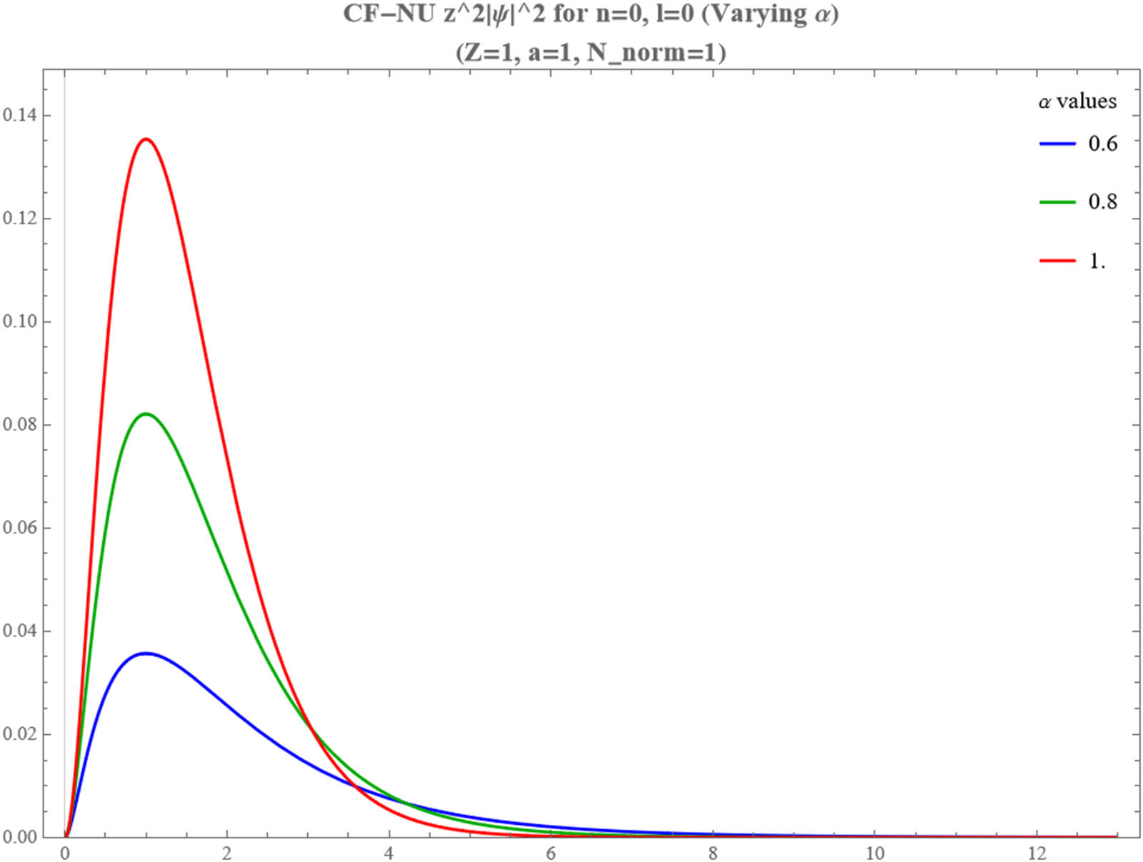
The obtained wavefunctions are illustrated in Figures 1, 2, 3, 4, 5, 6, which display both the radial wavefunction and the corresponding radial probability density for specific quantum states. Figure 1 presents an overlay comparison of the wavefunctions for the

Combined plot overlaying the radial wavefunction

Combined plot overlaying the radial probability density

CFNU radial wavefunction
CFNU radial probability density
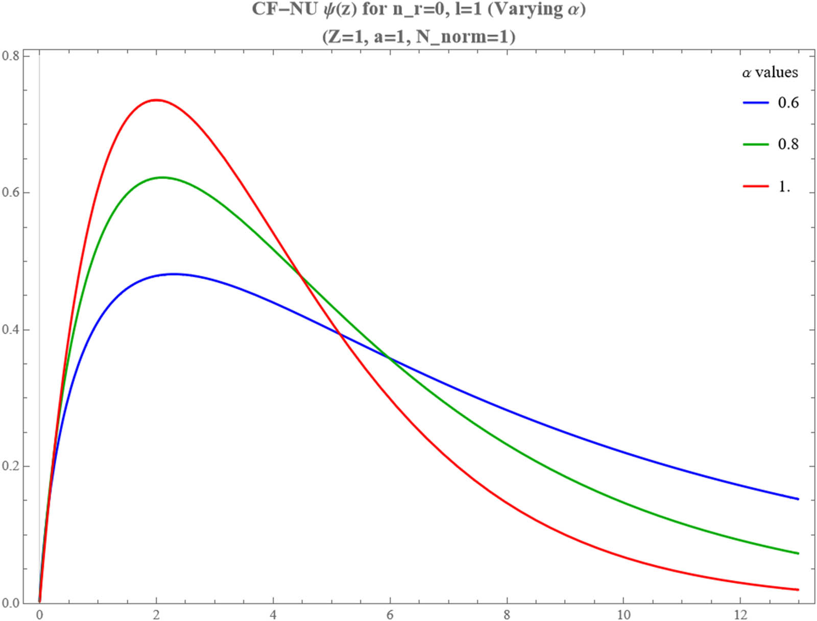
CFNU radial wavefunction
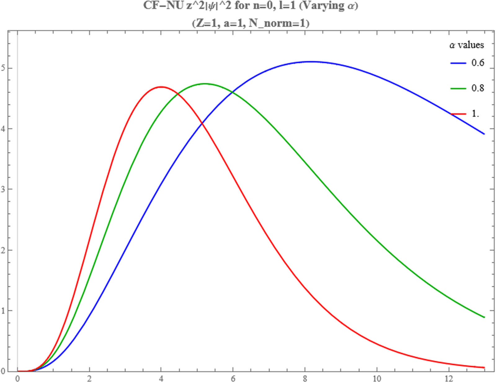
CFNU radial probability density
6 Significance of the fractional parameter
α
The fractional order
7 Practical applications and comparison
The CFNU method extends the utility of the established NU technique to the domain of fractional calculus, offering distinct advantages for specific classes of problems. While fundamental interactions in quantum mechanics are typically described by integer-order derivatives, effective field theories or models of quantum systems in complex environments (e.g., porous media, systems with long-range memory) may naturally lead to Schrödinger-like equations involving fractional derivatives [3]. In such scenarios, the CFNU method provides a robust analytical pathway to exact or approximate solutions that might be intractable with standard methods. Compared with purely numerical approaches for fractional differential equations, which can be computationally intensive and may present challenges regarding stability and convergence, analytical solutions derived via CFNU offer deeper physical insight into the system’s parameter dependencies and overall behavior. The method’s direct incorporation of the fractional order
8 Generalization to other potentials
The adaptability of the NU method and its conformable fractional extension (CF-NU) is not limited to the Coulomb potential. These algebraic techniques can be applied to a significant range of other physically relevant potentials, provided the corresponding Schrödinger equation (integer or fractional order) can be transformed into the canonical form required by the NU method. Examples include the harmonic oscillator, Morse potential, Hulthén potential, Rosen-Morse potential, Pöschl-Teller potential, and various empirical potentials used in molecular and nuclear physics [18,20]. The general procedure involves: (i) starting with the radial Schrödinger equation for the target potential, incorporating the conformable fractional derivative
9 Conclusion
In this study, we have investigated the exact bound state solutions of the radial Schrödinger equation for the Coulomb potential using the CFNU approach. The methodology allows for the systematic derivation of energy eigenvalues and unnormalized wavefunctions, where the fractional order
-
Funding information: This work was supported and funded by the Deanship of Scientific Research at Imam Mohammad Ibn Saud Islamic University (IMSIU) (grant number IMSIU-DDRSP2502).
-
Author contributions: All authors have accepted responsibility for the entire content of this manuscript and approved its submission.
-
Conflict of interest: The authors state no conflict of interest.
-
Data availability statement: Data sharing is not applicable to this article as no datasets were generated or analysed during the current study.
References
[1] Miller KS, Ross B. An introduction to the fractional calculus and fractional differential equations. New York: Wiley; 1993. Suche in Google Scholar
[2] Hilfer R. Applications of fractional calculus in physics. Singapore: World Scientific; 2000. 10.1142/9789812817747Suche in Google Scholar
[3] Herrmann R. Fractional calculus: an introduction for physicists. 3rd edition. Singapore: World Scientific; 2018. 10.1142/11107Suche in Google Scholar
[4] Podlubny I. Fractional: an introduction to fractional derivatives, fractional, to methods of their solution and some of their applications. San Diego: Elsevier; 1998. Suche in Google Scholar
[5] Khalil R, Horani MAH, Yousef A, Sababheh M. A new definition of fractional derivative. J Comput Appl Math. 2014;264:65–70. 10.1016/j.cam.2014.01.002Suche in Google Scholar
[6] Abdeljawad T. On conformable fractional calculus. J Comput Appl Math. 2015;279:57–66. 10.1016/j.cam.2014.10.016Suche in Google Scholar
[7] Yılmaz Karayer H, Demirhan D, Büyükkılıç F. Conformable fractional Nikiforov-Uvarov method. Commun Theor Phys. 2016;66:12–8. 10.1088/0253-6102/66/1/012Suche in Google Scholar
[8] Raddadi MH, Nahla AA, Abo-Kahla DAM. Quantized study for asymmetric two two-level atoms interacting with intensity-dependent coupling regime. Indian J Phys. 2023;97(5):1345–58. 10.1007/s12648-022-02497-8Suche in Google Scholar
[9] Abo-Kahla DAM. Long-lived quantum coherence and nonlinear properties of a two-dimensional semiconductor quantum well. J Opt Soc Am B. 2020;37(11):A96–109. 10.1364/JOSAB.393367Suche in Google Scholar
[10] Obada ASF, Abdel-Khalek S, Abo-Kahla DAM. The geometric phase of a two-level atom in a narrow-bandwidth squeezed vacuum. Optik. 2014;125(20):6335–9. 10.1016/j.ijleo.2014.06.153Suche in Google Scholar
[11] Abo-Kahla DAM. The pancharatnam phase of a three-level atom coupled to two systems of N-two level atoms. J Quantum Inf Sci. 2016;6(1):44–55. 10.4236/jqis.2016.61006Suche in Google Scholar
[12] Abo-Kahla D, Ahmed M, Makram-Allah A. Analytical solution of a three-level atom coupled to four systems of N-two-level atoms. Opt Rev. 2019;26(6):699–708. 10.1007/s10043-019-00559-7Suche in Google Scholar
[13] Abo-Kahla DAM, Ahmed MMA. Some studies of the interaction between N-two level atoms and three level atom. J Egypt Math Soc. 2016;24(3):487–91. 10.1016/j.joems.2015.10.004Suche in Google Scholar
[14] Nikiforov AF, Uvarov VB. Special functions of mathematical physics: A unified introduction with applications. Birkhäuser, Basel; 1988. 10.1007/978-1-4757-1595-8Suche in Google Scholar
[15] Al-Hawamdeh MA, Akour AN, Jaradat EK, Jaradat OK. Involving Nikiforov-Uvarov method in Schrodinger equation obtaining Hartmann potential. East Eur J Phys. 2023;2(2):117–23. 10.26565/2312-4334-2023-2-10Suche in Google Scholar
[16] Akour AN, Jaradat EK, Tarawneh SR, Jaradat OK. A new vision on Schrödinger equation using position dependent mass concerning modified Hylleraas-Hulthén potential expanded by Nikiforov-Uvarov method. Int J Multiphys. 2024;18(2):553–64. Suche in Google Scholar
[17] Jaradat EK, Tarawneh S, Aloqali A, Ajoor M, Hijjawi R, Jaradat O. Position-dependent mass Schrödinger equation for the q-deformed Woods-Saxson plus hyperbolic tangent potential. Int J Adv Appl Sci. 2024;11(8):44–50. 10.21833/ijaas.2024.08.005Suche in Google Scholar
[18] Gordillo-Núñez G, Alvarez-Nodarse R, Quintero NR. The complete solution of the Schrödinger equation with the Rosen-Morse type potential via the Nikiforov-Uvarov method. Phys D Nonl Phenom. 2024;458:134008. 10.1016/j.physd.2023.134008Suche in Google Scholar
[19] Berkdemir C. Application of the Nikiforov–Uvarov. In: Theoretical concepts of quantum mechanics. London: IntechOpen; 2012. p. 225. 10.5772/33510Suche in Google Scholar
[20] Egrifes H, Sever R. Bound-state solutions of the Klein-Gordon equation for the generalized PT-symmetric Hulthén potential. Int J Theor Phys. 2007;46(4):935–44. 10.1007/s10773-006-9251-8Suche in Google Scholar
[21] Motavalli H, Akbarieh AR. Exact solutions of the Klein-Gordon equation for the Scarf-type potential via Nikiforov-Uvarov method. Int J Theor Phys. 2010;49:379–89. 10.1007/s10773-010-0277-6Suche in Google Scholar
[22] Alvarez-Castillo DE, Kirchbach M. Exact spectrum and wave functions of the hyperbolic Scarf potential in terms of finite Romanovski polynomials. Rev Mex Fis. 2011;57:385–92. Suche in Google Scholar
[23] Ellis L, Ellis I, Koutschan C, Suslov SK. On Potentials Integrated by the Nikiforov-Uvarov method [Technical Report RICAM-Report 2023-11]. Research Institute for Symbolic Computation (RICAM); 2023. Suche in Google Scholar
[24] Dong S-H. Factorization method in quantum mechanics. Dordrecht: Springer; 2007. 10.1007/978-1-4020-5796-0Suche in Google Scholar
[25] Flügge S. Practical quantum mechanics. Berlin: Springer Science & Business Media; 2012. Suche in Google Scholar
© 2025 the author(s), published by De Gruyter
This work is licensed under the Creative Commons Attribution 4.0 International License.
Artikel in diesem Heft
- Research Articles
- Single-step fabrication of Ag2S/poly-2-mercaptoaniline nanoribbon photocathodes for green hydrogen generation from artificial and natural red-sea water
- Abundant new interaction solutions and nonlinear dynamics for the (3+1)-dimensional Hirota–Satsuma–Ito-like equation
- A novel gold and SiO2 material based planar 5-element high HPBW end-fire antenna array for 300 GHz applications
- Explicit exact solutions and bifurcation analysis for the mZK equation with truncated M-fractional derivatives utilizing two reliable methods
- Optical and laser damage resistance: Role of periodic cylindrical surfaces
- Numerical study of flow and heat transfer in the air-side metal foam partially filled channels of panel-type radiator under forced convection
- Water-based hybrid nanofluid flow containing CNT nanoparticles over an extending surface with velocity slips, thermal convective, and zero-mass flux conditions
- Dynamical wave structures for some diffusion--reaction equations with quadratic and quartic nonlinearities
- Solving an isotropic grey matter tumour model via a heat transfer equation
- Study on the penetration protection of a fiber-reinforced composite structure with CNTs/GFP clip STF/3DKevlar
- Influence of Hall current and acoustic pressure on nanostructured DPL thermoelastic plates under ramp heating in a double-temperature model
- Applications of the Belousov–Zhabotinsky reaction–diffusion system: Analytical and numerical approaches
- AC electroosmotic flow of Maxwell fluid in a pH-regulated parallel-plate silica nanochannel
- Interpreting optical effects with relativistic transformations adopting one-way synchronization to conserve simultaneity and space–time continuity
- Modeling and analysis of quantum communication channel in airborne platforms with boundary layer effects
- Theoretical and numerical investigation of a memristor system with a piecewise memductance under fractal–fractional derivatives
- Tuning the structure and electro-optical properties of α-Cr2O3 films by heat treatment/La doping for optoelectronic applications
- High-speed multi-spectral explosion temperature measurement using golden-section accelerated Pearson correlation algorithm
- Dynamic behavior and modulation instability of the generalized coupled fractional nonlinear Helmholtz equation with cubic–quintic term
- Study on the duration of laser-induced air plasma flash near thin film surface
- Exploring the dynamics of fractional-order nonlinear dispersive wave system through homotopy technique
- The mechanism of carbon monoxide fluorescence inside a femtosecond laser-induced plasma
- Numerical solution of a nonconstant coefficient advection diffusion equation in an irregular domain and analyses of numerical dispersion and dissipation
- Numerical examination of the chemically reactive MHD flow of hybrid nanofluids over a two-dimensional stretching surface with the Cattaneo–Christov model and slip conditions
- Impacts of sinusoidal heat flux and embraced heated rectangular cavity on natural convection within a square enclosure partially filled with porous medium and Casson-hybrid nanofluid
- Stability analysis of unsteady ternary nanofluid flow past a stretching/shrinking wedge
- Solitonic wave solutions of a Hamiltonian nonlinear atom chain model through the Hirota bilinear transformation method
- Bilinear form and soltion solutions for (3+1)-dimensional negative-order KdV-CBS equation
- Solitary chirp pulses and soliton control for variable coefficients cubic–quintic nonlinear Schrödinger equation in nonuniform management system
- Influence of decaying heat source and temperature-dependent thermal conductivity on photo-hydro-elasto semiconductor media
- Dissipative disorder optimization in the radiative thin film flow of partially ionized non-Newtonian hybrid nanofluid with second-order slip condition
- Bifurcation, chaotic behavior, and traveling wave solutions for the fractional (4+1)-dimensional Davey–Stewartson–Kadomtsev–Petviashvili model
- New investigation on soliton solutions of two nonlinear PDEs in mathematical physics with a dynamical property: Bifurcation analysis
- Mathematical analysis of nanoparticle type and volume fraction on heat transfer efficiency of nanofluids
- Creation of single-wing Lorenz-like attractors via a ten-ninths-degree term
- Optical soliton solutions, bifurcation analysis, chaotic behaviors of nonlinear Schrödinger equation and modulation instability in optical fiber
- Chaotic dynamics and some solutions for the (n + 1)-dimensional modified Zakharov–Kuznetsov equation in plasma physics
- Fractal formation and chaotic soliton phenomena in nonlinear conformable Heisenberg ferromagnetic spin chain equation
- Single-step fabrication of Mn(iv) oxide-Mn(ii) sulfide/poly-2-mercaptoaniline porous network nanocomposite for pseudo-supercapacitors and charge storage
- Novel constructed dynamical analytical solutions and conserved quantities of the new (2+1)-dimensional KdV model describing acoustic wave propagation
- Tavis–Cummings model in the presence of a deformed field and time-dependent coupling
- Spinning dynamics of stress-dependent viscosity of generalized Cross-nonlinear materials affected by gravitationally swirling disk
- Design and prediction of high optical density photovoltaic polymers using machine learning-DFT studies
- Robust control and preservation of quantum steering, nonlocality, and coherence in open atomic systems
- Coating thickness and process efficiency of reverse roll coating using a magnetized hybrid nanomaterial flow
- Dynamic analysis, circuit realization, and its synchronization of a new chaotic hyperjerk system
- Decoherence of steerability and coherence dynamics induced by nonlinear qubit–cavity interactions
- Finite element analysis of turbulent thermal enhancement in grooved channels with flat- and plus-shaped fins
- Modulational instability and associated ion-acoustic modulated envelope solitons in a quantum plasma having ion beams
- Statistical inference of constant-stress partially accelerated life tests under type II generalized hybrid censored data from Burr III distribution
- On solutions of the Dirac equation for 1D hydrogenic atoms or ions
- Entropy optimization for chemically reactive magnetized unsteady thin film hybrid nanofluid flow on inclined surface subject to nonlinear mixed convection and variable temperature
- Stability analysis, circuit simulation, and color image encryption of a novel four-dimensional hyperchaotic model with hidden and self-excited attractors
- A high-accuracy exponential time integration scheme for the Darcy–Forchheimer Williamson fluid flow with temperature-dependent conductivity
- Novel analysis of fractional regularized long-wave equation in plasma dynamics
- Development of a photoelectrode based on a bismuth(iii) oxyiodide/intercalated iodide-poly(1H-pyrrole) rough spherical nanocomposite for green hydrogen generation
- Investigation of solar radiation effects on the energy performance of the (Al2O3–CuO–Cu)/H2O ternary nanofluidic system through a convectively heated cylinder
- Quantum resources for a system of two atoms interacting with a deformed field in the presence of intensity-dependent coupling
- Studying bifurcations and chaotic dynamics in the generalized hyperelastic-rod wave equation through Hamiltonian mechanics
- A new numerical technique for the solution of time-fractional nonlinear Klein–Gordon equation involving Atangana–Baleanu derivative using cubic B-spline functions
- Interaction solutions of high-order breathers and lumps for a (3+1)-dimensional conformable fractional potential-YTSF-like model
- Hydraulic fracturing radioactive source tracing technology based on hydraulic fracturing tracing mechanics model
- Numerical solution and stability analysis of non-Newtonian hybrid nanofluid flow subject to exponential heat source/sink over a Riga sheet
- Numerical investigation of mixed convection and viscous dissipation in couple stress nanofluid flow: A merged Adomian decomposition method and Mohand transform
- Effectual quintic B-spline functions for solving the time fractional coupled Boussinesq–Burgers equation arising in shallow water waves
- Analysis of MHD hybrid nanofluid flow over cone and wedge with exponential and thermal heat source and activation energy
- Solitons and travelling waves structure for M-fractional Kairat-II equation using three explicit methods
- Impact of nanoparticle shapes on the heat transfer properties of Cu and CuO nanofluids flowing over a stretching surface with slip effects: A computational study
- Computational simulation of heat transfer and nanofluid flow for two-sided lid-driven square cavity under the influence of magnetic field
- Irreversibility analysis of a bioconvective two-phase nanofluid in a Maxwell (non-Newtonian) flow induced by a rotating disk with thermal radiation
- Hydrodynamic and sensitivity analysis of a polymeric calendering process for non-Newtonian fluids with temperature-dependent viscosity
- Exploring the peakon solitons molecules and solitary wave structure to the nonlinear damped Kortewege–de Vries equation through efficient technique
- Modeling and heat transfer analysis of magnetized hybrid micropolar blood-based nanofluid flow in Darcy–Forchheimer porous stenosis narrow arteries
- Activation energy and cross-diffusion effects on 3D rotating nanofluid flow in a Darcy–Forchheimer porous medium with radiation and convective heating
- Insights into chemical reactions occurring in generalized nanomaterials due to spinning surface with melting constraints
- Influence of a magnetic field on double-porosity photo-thermoelastic materials under Lord–Shulman theory
- Soliton-like solutions for a nonlinear doubly dispersive equation in an elastic Murnaghan's rod via Hirota's bilinear method
- Analytical and numerical investigation of exact wave patterns and chaotic dynamics in the extended improved Boussinesq equation
- Nonclassical correlation dynamics of Heisenberg XYZ states with (x, y)-spin--orbit interaction, x-magnetic field, and intrinsic decoherence effects
- Exact traveling wave and soliton solutions for chemotaxis model and (3+1)-dimensional Boiti–Leon–Manna–Pempinelli equation
- Unveiling the transformative role of samarium in ZnO: Exploring structural and optical modifications for advanced functional applications
- On the derivation of solitary wave solutions for the time-fractional Rosenau equation through two analytical techniques
- Analyzing the role of length and radius of MWCNTs in a nanofluid flow influenced by variable thermal conductivity and viscosity considering Marangoni convection
- Advanced mathematical analysis of heat and mass transfer in oscillatory micropolar bio-nanofluid flows via peristaltic waves and electroosmotic effects
- Exact bound state solutions of the radial Schrödinger equation for the Coulomb potential by conformable Nikiforov–Uvarov approach
- Some anisotropic and perfect fluid plane symmetric solutions of Einstein's field equations using killing symmetries
- Nonlinear dynamics of the dissipative ion-acoustic solitary waves in anisotropic rotating magnetoplasmas
- Curves in multiplicative equiaffine plane
- Exact solution of the three-dimensional (3D) Z2 lattice gauge theory
- Propagation properties of Airyprime pulses in relaxing nonlinear media
- Symbolic computation: Analytical solutions and dynamics of a shallow water wave equation in coastal engineering
- Wave propagation in nonlocal piezo-photo-hygrothermoelastic semiconductors subjected to heat and moisture flux
- Comparative reaction dynamics in rotating nanofluid systems: Quartic and cubic kinetics under MHD influence
- Laplace transform technique and probabilistic analysis-based hypothesis testing in medical and engineering applications
- Physical properties of ternary chloro-perovskites KTCl3 (T = Ge, Al) for optoelectronic applications
- Gravitational length stretching: Curvature-induced modulation of quantum probability densities
- The search for the cosmological cold dark matter axion – A new refined narrow mass window and detection scheme
- A comparative study of quantum resources in bipartite Lipkin–Meshkov–Glick model under DM interaction and Zeeman splitting
- PbO-doped K2O–BaO–Al2O3–B2O3–TeO2-glasses: Mechanical and shielding efficacy
- Nanospherical arsenic(iii) oxoiodide/iodide-intercalated poly(N-methylpyrrole) composite synthesis for broad-spectrum optical detection
- Sine power Burr X distribution with estimation and applications in physics and other fields
- Numerical modeling of enhanced reactive oxygen plasma in pulsed laser deposition of metal oxide thin films
- Dynamical analyses and dispersive soliton solutions to the nonlinear fractional model in stratified fluids
- Computation of exact analytical soliton solutions and their dynamics in advanced optical system
- An innovative approximation concerning the diffusion and electrical conductivity tensor at critical altitudes within the F-region of ionospheric plasma at low latitudes
- An analytical investigation to the (3+1)-dimensional Yu–Toda–Sassa–Fukuyama equation with dynamical analysis: Bifurcation
- Swirling-annular-flow-induced instability of a micro shell considering Knudsen number and viscosity effects
- Review Article
- Examination of the gamma radiation shielding properties of different clay and sand materials in the Adrar region
- Erratum
- Erratum to “On Soliton structures in optical fiber communications with Kundu–Mukherjee–Naskar model (Open Physics 2021;19:679–682)”
- Special Issue on Fundamental Physics from Atoms to Cosmos - Part II
- Possible explanation for the neutron lifetime puzzle
- Special Issue on Nanomaterial utilization and structural optimization - Part III
- Numerical investigation on fluid-thermal-electric performance of a thermoelectric-integrated helically coiled tube heat exchanger for coal mine air cooling
- Special Issue on Nonlinear Dynamics and Chaos in Physical Systems
- Analysis of the fractional relativistic isothermal gas sphere with application to neutron stars
- Abundant wave symmetries in the (3+1)-dimensional Chafee–Infante equation through the Hirota bilinear transformation technique
- Successive midpoint method for fractional differential equations with nonlocal kernels: Error analysis, stability, and applications
- Novel exact solitons to the fractional modified mixed-Korteweg--de Vries model with a stability analysis