
Finite element analysis of turbulent thermal enhancement in grooved channels with flat- and plus-shaped fins
-
Younes Menni
 ,
Noureddine Kaid
,
Noureddine Kaid

Abstract
This study numerically investigates turbulent convective heat transfer (HT) in a rectangular channel enhanced with fins and grooves using the finite element method and the standard k–ε turbulence model. The novelty lies in the combined evaluation of rectangular, trapezoidal, and triangular grooves by varying the b/c ratio from 1.0 to 0, along with a systematic optimization of plus (+) and flat fin heights. Among six groove configurations, the b/c = 0.75 trapezoidal groove produced the highest temperature increase (ΔT = T out − T inlet) of 16.54% improvement over the baseline ungrooved channel. Through additional optimization, raising both fin types to 1.50 h was found to provide the optimal thermal performance with an outlet temperature of 51.17°C and a 146.88% improvement in ΔT compared to the baseline. These results highlight the large synergistic effect of groove geometry and fin height optimization, yielding an effective design strategy for enhancing HT in solar heat exchanger devices.
1 Introduction
The increasing demands from various parts of the world regarding thermally sustainable and renewable energy sources have put pressure on the latest developments in the field of thermophysics, especially on how efficiently the energy from the sun can be utilized. Solar air heaters (SAHs) comprise one of the key players in this field due to their simple design and relative inexpensiveness. Their uses span a wide range of applications, starting from heating space to the drying of agricultural products. Their optimum design and operational parameters improve their efficiency manifold. Experiments have been carried out continuously by researchers to improve performance in HE channels by making various modifications. Most of the modifications incorporate the use of fins, baffles, and other turbulators. Singh and Dhiman [1] conducted the study with the double-pass SAHs with fins and baffles. Conclusions drawn from the study show that the increased mass flow rate and recycle ratio enhance efficiency greatly due to an increase in fluid velocity, whereas baffles enhance heat transfer (HT). The studies conducted by Eiamsa-Ard et al. [2] were related to the rectangular channels having square-wing perforated V-type baffles. They concluded that the angle of attack at 45° provided maximum thermal performance factor, while the angle of 22.5° gave maximum HT augmentation.
Entropy generation in a three-dimensional channel with perforated transverse twisted baffles was numerically studied by Esmaeili and Rashidi [3], using an alumina/water nanofluid. Their results showed that increasing the number of holes in baffles increased the HT coefficient and reduced the pressure loss; the best performance was obtained for four holes and a pitch of 540° at an angle of 45°. Lopez et al. [4] conducted experiments on laminar forced convective HT in baffled channels. They showed that the HT enhancement as a function of pressure drop depends on the Reynolds (Re) and Prandtl (Pr) numbers. Santos and de Lemos [5] performed numerical simulations with both solid and porous baffles in laminar flow. The final deduction was that there is no enhancement of HT by low-porosity baffles compared to solid ones.
Da Silva Miranda and Anand [6] concluded that solid baffles produced higher HT enhancement compared to porous baffles in laminar forced convection, especially at larger Re numbers and thermal conductivity ratios. Yang et al. [7] conducted optimization of porous pin fins with design of experiments, genetic algorithms, and computational fluid dynamics (CFD), achieving significant enhancements in HT and fluid flow (FF). Kheradmand-Laleh et al. [8] showed that for some Darcy numbers and aspect ratios, the use of a semi-porous fin, comprising porous and solid parts, improved HT and reduced the pressure penalties.
Venkatesh and Meenakshi Reddy [9] compared the teardrop pin fins in turbine trailing edge cooling channels to the circular fins and found that the HT enhancement was 10.45%, while a reduction of 54.6% was seen in pressure drop. Perão et al. [10] evaluated that in the finned channel, the pressure drops were found to be smaller and HT rates are higher for staggered fin arrangements by comparison with in-line fins. Aouissi and Chabane [11] showed that for solar air collectors, the average Nusselt number (Nu) and friction coefficient (Cf) increased with an increase in the number of rectangular baffles.
Chamoli and Thakur [12] highlighted that baffles enhance the HT and thermal efficiency in SAHs most significantly, while the optimal geometrical design was determined by the flow attack angle and the form of baffles. Chabane et al. [13] showed that the best thermal efficiency could be achieved by applying rectangular baffles disposed perpendicularly to airflow at median and transversal locations. Jain et al. [14] found that discrete V-shaped perforated baffles enhanced Nu and Cf, thereby achieving a thermohydraulic performance parameter of 2.24 at optimality.
Mukilarasan et al. [15] demonstrated that a 45°: ± 45°: 45° baffle arrangement improved the HT in shell and tube HEs without changing the design modification. Henniche and Korichi [16] investigated that self-sustained oscillatory flow in asymmetrically heated baffled channels develops the HT at moderate Re number, whereas these modifications result in increased power consumption of pumping. Wang et al. [17] compared the helical baffles with conventional segmental baffles for enhancing the performance of shell-and-tube HEs.
Sharma et al. [18] illustrated that sine wave baffles in SAHs resulted in the enhancement of thermal efficiency up to 78% along with an effective efficiency of 70.8%. Naqvi and Wang [19] showed that the utilization of porous media enhanced HT in shell-and-tube HEs with different baffle design at the expense of a minimal pressure drop penalty, especially for anti-vibration configurations. Joye and Côté [20] indicated that helical fins enhance HT coefficients by 40–50%, while the longitudinal fins have surprisingly increased it by 260% due to some cross-flow effect.
Thomas Renald et al. [21] conducted a study concerning wavy fins on a triangular duct SAH. It is noticed that the higher the amplitude ratio of the fin, the more thermally efficient it is, and here, it reaches 85%. Michael Joseph Stalin et al. [22] presented that prismatic triangular SAHs with longitudinal fins and rib turbulators optimized for high thermal performance substantially enhance it. Wang et al. [23] concluded that among unsymmetrical helical baffle geometries in shell-and-tube HEs, a quarter one provides an optimal compromise between low flow resistance and moderate HT efficiency.
Menni et al. [24] aimed at the goal of combining baffles and nanofluids to achieve a significant enhancement in the thermal efficiency in HEs using multi-walled carbon nanotubes as the working fluid, especially upon the use of vertical baffles. Fourar and Benmachiche [25] came up with an innovation on the traditional circular fins by introducing a V-shaped cut that attained substantial weight reductions and an enhanced HT rate. Sharma et al. [26] concerned mixed convection in grooved channels with central adiabatic baffles, in which considerable HT gain was reported, especially in the mixed convection regime.
Yang et al. [27] conducted the experimental investigation of the lantern-shaped pin fins to cool gas turbines and mentioned that with a higher sphere-to-pin diameter ratio, the thermal performance increased noticeably at the higher Re number. Chabane et al. [28] researched the enhancement in SAH thermal performance by integrating several baffles within these; the arrangement and the number of baffles were identified to have a potential impact on the optimization of efficiency. Tsay et al. [29] studied mixed convection in baffle-mounted ducts around heated blocks and found that the strategic positioning of baffles can significantly increase Nu numbers and hence the system HT rates.
Facas [30] carried out an analysis to demonstrate that the use of baffles in a Darcy-flow governed porous medium results in increased energy efficiency, hence increasing the Nu number. The performance gain was related to the Rayleigh number, Ra, burial depth, and baffle length. Ahmadinejad et al. [31] numerically investigated a photovoltaic thermal system with a sinusoidal fin. They indicated high energy and exergy promotion using the Cu/water nanofluid under several variable conditions, including favorable flow rates and cooler inflows. According to Shaeri and Jen [32], there are higher HT rates and lower drag at higher porosities, and hence, less resistance is obtained with fewer perforations.
Demartini et al. [33] performed numerical and experimental analyses of turbulent flow through baffle-structured channels, and their work is quite fundamental to understanding the dynamics of flow in complicated geometries. Kedar et al. [34], on the other hand, presented a study related to SAHs in industries. Passive features such as baffles and fins are used here in order to overcome the air’s poor characteristics of thermodynamics; hence, the maximum efficiency for such systems can be achieved at 81.9%. Improvement in thermal efficiency up to 14.7% for jet plate SAHs may be included using continuous fins, especially for high Re number values, as reported by Goel and Singh [35].
Berber et al. [36] showed that curved winglet vortex generators show that VGs significantly enhance the Nu number in rectangular channels; for increased attack angles, the HT enhancement is as high as 476.08% over plain tubes. Ishaq et al. [37] optimized trapezoidal fins in elliptical-core HEs regarding fin number, height, and radius ratio; significant enhancements in HT performance are present. Other studies used various HT techniques, such as the analysis of MHD nanofluid convection and phase change in a corrugated channel with elastic partitions by Omri et al. [38], the optimization of a cooling system with perforated porous inserts and POD modeling by Selimefendigil et al. [39], and the investigation of fluid–structure interactions in CNT–water nanofluid convection in a microchannel with elastic fins under periodic inlet flow by Ben Said et al. [40].
Si et al. [41] demonstrated that the application of VGs with semi-detached inclined trapezoidal wings in transformer radiator channels enhances HT by as much as 8.9% compared to a standard design. The optimal separation height is e/(0.5H) = 0.3 and inclination angles between 30° and 60°. Wang et al. [42] showed that a trapezoidal rib combined with a 6 vol% CuO–EGW nanofluid improved the Nu number by 135.8% with respect to smooth tubes, where the optimum was at a rib angle of 75° and a PEC of 1.64.
On the other hand, the use of machine learning and deep learning models has come into prominence for the prediction and optimization of complex HT mechanisms in advanced fluid systems. Kumar et al. [43] used a support vector machine for the classification of HT rates in tri-hybrid nanofluids in a 3D stretching surface with accurate predictions under various temperatures and suction impacts. In a concurrent study, Kumar et al. [44] used response surface methodology and deep learning to forecast and optimize HT in water-based hybrid nanofluid flows of thin films with effective performance mapping. Moreover, Kumar et al. [45] combined deep neural networks and CFD to model convective HT in dusty FF with improved prediction accuracy for complex HT conditions.
1.1 Motivation
The growing global need for the utilization of renewable energy sources acknowledges the need to develop technologies to harness such resources. Solar HEs are an integral component of solar thermal systems, and their efficiency needs to be optimized to maximize energy efficiency. Such technologies will play a pivotal role in accelerating the phase out of fossil fuels and combating climate change, in addition to the sustainable development goals.
1.2 Aim of the study
The aim of this research is to investigate comprehensively the hydrothermal behavior of fin-and-groove-integrated solar HEs. Through the application of the finite element method (FEM), the study employs the standard
1.3 Originality
The originality of this study lies in its exhaustive exploration of blended fin and groove geometries by FEM and turbulence modeling. Previous studies have explored the effects of fins or grooves in separation, while this one targets their combined impact on flow turbulence and thermal behavior in HE channels, a new aspect of solar thermal system design.
1.4 Significance and contribution
By identifying geometrical configurations that improve thermal performance, this study is geared toward high-efficiency solar HE improvement. Findings from this research encourage improved solar energy systems, thus encouraging innovation in renewable technologies and global efforts toward the sustainability of energy and maximum utilization of resources.
2 Materials and methods
2.1 Study description
The hydrothermal performance is studied numerically in the present research work for a rectangular channel fitted with a different groove and fin configuration. Figure 1 shows the geometrical configuration of the rectangular channel with grooves and fins that are installed to augment HT by forced convection.

Schematic diagram of the rectangular channel with varying groove and fin configurations: (a) Case 1: ungrooved finned channel; (b) Case 2: finned channel with rectangular grooves: b/c = 1; (c) Case 3: finned channel with trapezoïdal grooves: b/c = 0.25, 0.50 and 0.75; and (d) Case 4: finned channel with triangular grooves: b/c = 0.
Figure 1(a) presents a design configuration involving the placing of fins in both “+” and flat shapes, each contributing to enhancing turbulence in flow and thereby raising the effectiveness of HT. Figure 1(b)–(d) extends the configuration of Figure 1(a) by adding grooves of various geometries on both walls of the channel, positioned opposite to each fin. These grooves are for enhancing the hydrodynamic performance of the channel by disrupting the boundary layer flow and mixing, hence promoting strong thermal interaction between the fluid and channel surfaces. The integration of such geometric features tries to make the overall thermal efficiency of the system much better.
2.1.1 Influence of groove geometry
In the first stage of this simulation, these grooves are designed to have different shapes, starting from rectangular with b/c ratio of 1 in case 2, passing through trapezoidal forms with b/c ratios of 0.75 in case 3i, 0.50 in case 3ii, and 0.25 in case 3iii, up to triangular with b/c ratio of 0 in case 4.
2.1.2 Influence of fin geometry
In the second stage of this simulation, after selecting the best grooved channel, the inquiry shifts to the fin heights using a parametric study systematically.
First test: The height of the first fin “+,” which was studied incrementally from 0.25 to 1.50 h, was done keeping the second fin keeping h constant.
Second assessment: The configuration is reversed, with the first fin’s height fixed at h, and the height of the second fin (flat) varied between 0.25 and 1.50 h.
Third analysis: The height of both fins is varied simultaneously in the range 0.25–1.50 h to investigate the coupled effects.
Optimal fin dimensions for each case are identified based on the performance criterion representing the average outlet temperature (T out). A comparison among these optimal configurations is then carried out to arrive at the selection of the best design.
All the dimensions of the channel, L, L inlet, L exit, H, D h, h, and e are taken from the experiment conducted by Demartini et al. [33], while the groove dimensions, a, b, c, and d, together with the “+” fin dimension, “h,” are proposed for this study.
2.2 Material properties
Air is chosen as the working fluid since its fluid dynamic and thermophysical characteristics are well-documented under normal ambient conditions. Due to its thorough documentation and predictable behavior, it is widely accepted as a representative medium for air-based thermal engineering applications with heating and cooling processes. Here, the thermophysical characteristics of air are obtained from COMSOL Multiphysics (version 5.0) [47]. The temperature-dependent properties of air are presented in Table 1. For clearer representative presentation, Figure 2(a)–(d) shows the dependence of air properties on temperature. Further, the values at 300 K are emphasized by projecting them onto the temperature axis to facilitate reference under standard conditions.
Temperature-dependent thermophysical properties of air used in the simulations
| Property | Function | Unit |
|---|---|---|
| Density (
|
|
kg/m3 |
| Thermal conductivity (
|
|
W/m K |
| Heat capacity at constant pressure (
|
|
J/kg K |
| Viscosity (
|
|
kg/m s |
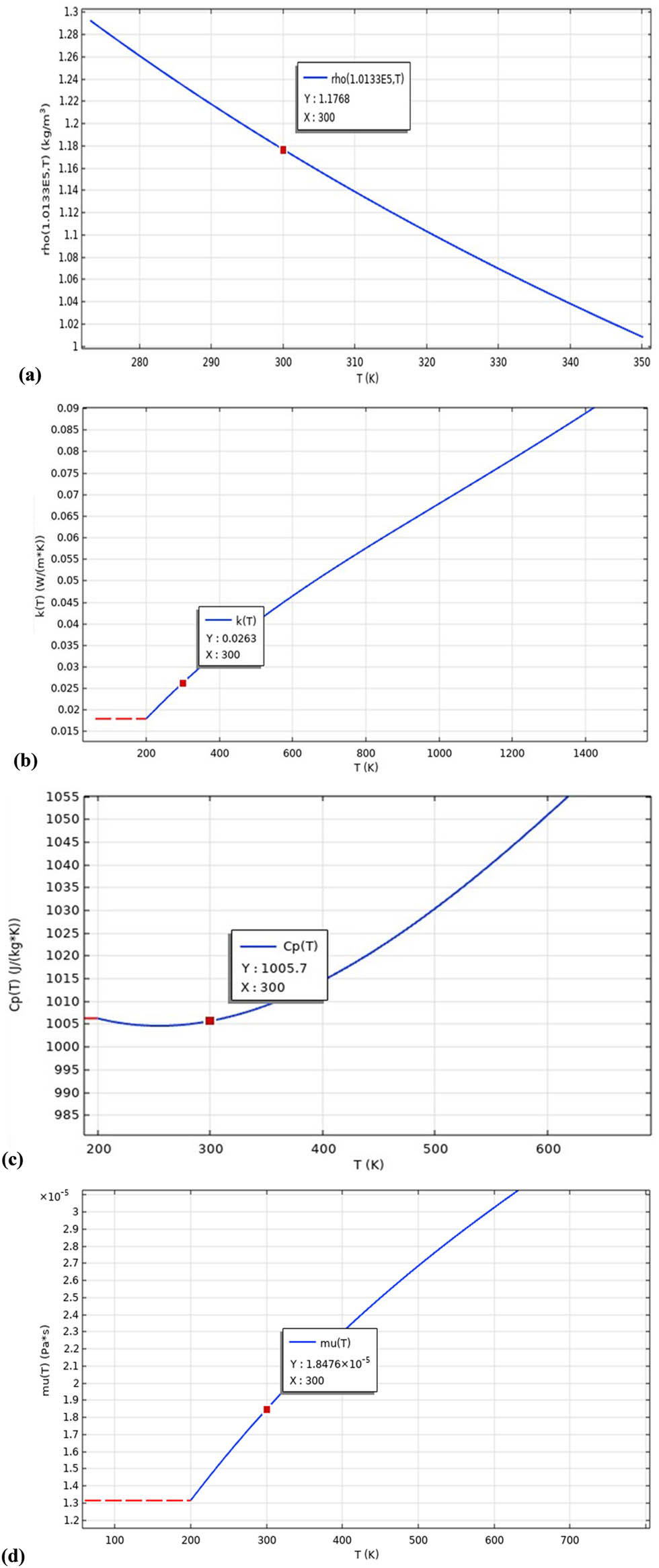
Temperature-dependent thermophysical properties of air: (a) density, (b) thermal conductivity, (c) heat capacity at constant pressure, and (d) viscosity.
Aluminum (Al) is used for the geometry of the channel, which was selected on the grounds of having high thermal conductivity, low mass, and excellent mechanical strength. Such properties make Al most suitable to enhance the efficiency of HT while it is capable of withstanding structural integrity under heat load. Thermophysical properties of aluminum at 300 K, as utilized within this work, are presented in Table 2 and retrieved from COMSOL Multiphysics (version 5.0) [47].
Thermophysical properties of solid (Al) at 300 K
| Density | Heat capacity at constant pressure | Thermal conductivity |
|---|---|---|
| ρ s (kg/m3) | Cps (J/kg K) | k s (W/m K) |
| 2,700 | 900 | 238 |
2.3 Boundary conditions and governing equations
Some of the applied boundary conditions include the following:
Constant temperature boundary: The fins and grooves, as well as the upper and lower walls of the channel, are assumed to be at a fixed temperature of 375 K, as conducted by Siddiqui [48].
Velocity inlet and pressure outlet: The inlet is given a uniform velocity profile, and the outlet is set under atmospheric pressure, as reported in Demartini et al. [33].
No-slip and impermeability conditions: No-slip and impermeability conditions are imposed on all solid–fluid interfaces, as simulated by Demartini et al. [33], for proper modeling of interaction between air with the channel surfaces.
In this work, hydrothermal performance in a rectangular channel with various groove and fin configurations is simulated using the FEM [49] on COMSOL Multiphysics 5.0 [47]. This numerical platform is used to comprehensively study FF and HT behavior influenced by internal surface characteristics. The standard
The flow and HT equations are derived from the conservation of mass, momentum, and energy, along with the turbulence model. The governing RANS equations for two-dimensional, incompressible, Newtonian FF are given by [33]:
Continuity
Momentum
where
The Reynolds stress term
where
Energy
The energy equation is given as [51]
where
Standard
In the selected model, the equations for turbulent kinetic energy (
The turbulence model uses the following empirical coefficients:
The Reynolds number (Re) is given by
where U 0 is the inlet flow velocity, D h is the channel hydraulic diameter, and μ is the dynamic viscosity of the fluid.
2.4 Verification of the mesh
Variable meshing has been used to discretize the computational domain to ensure high resolution in steep gradient regions, for example, regions close to fins and grooves (Figure 3).

Non-uniform mesh distribution in the computational domain for enhanced resolution near fins and grooves: (a) Case 1, (b) Case 2, (c) Case 3i, (d) Case 3ii, (e) Case 3iii, and (f) Case 4.
These are areas that need finer grid meshing in order to capture the flow separation, re-attachment, and hence, improved distribution. This is quite necessary in resolving the disruption of the boundary layer and thus the ensuing improvement in HT performance. The near-wall mesh refinement includes the resolved boundary layers along channel walls, fins, and grooves by inflation layers with a growth rate carefully selected to balance the computational cost against the accuracy in capturing thermal and velocity boundary layers with enough detail.
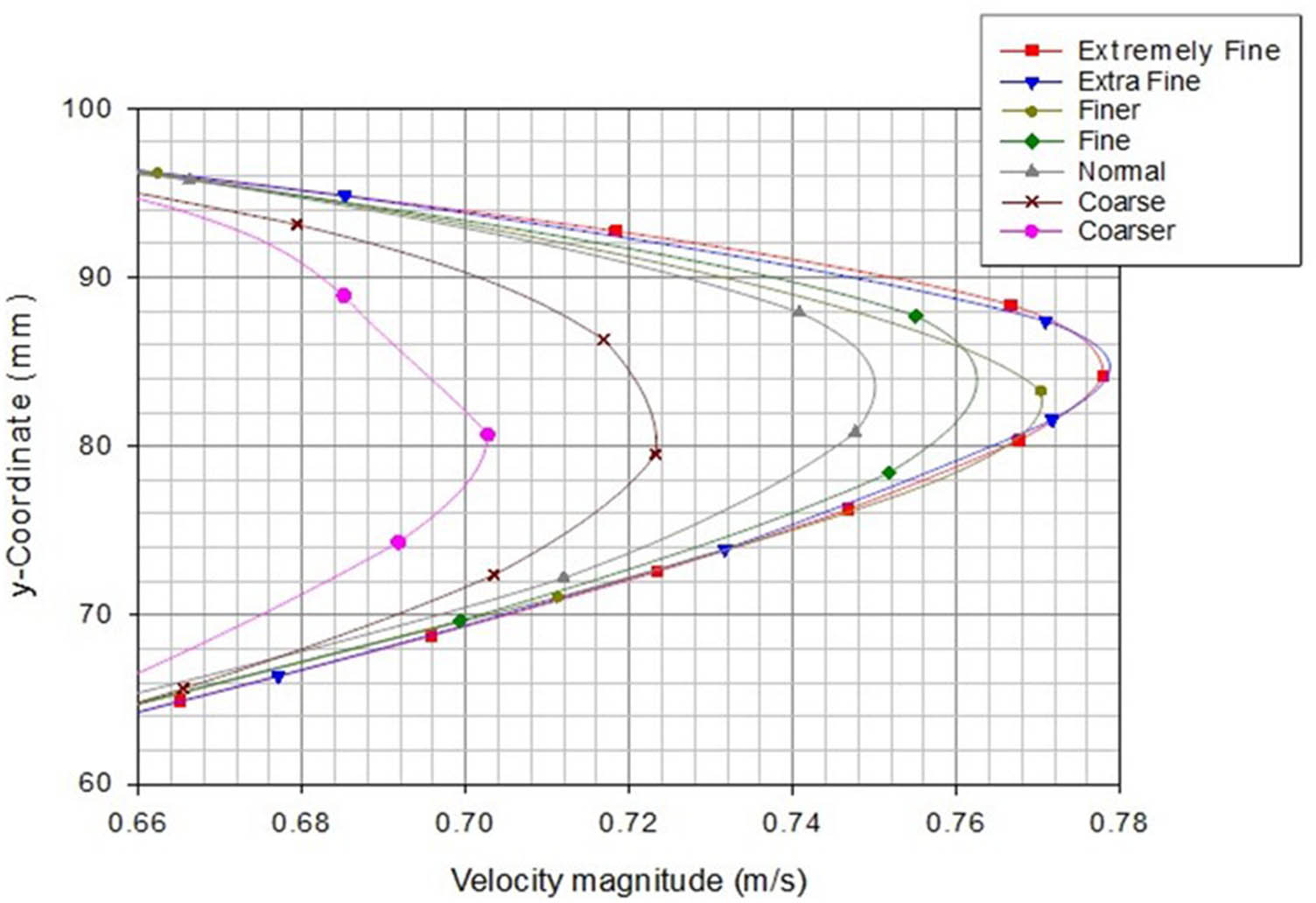
In the grid-independent study, the suitable mesh density was determined such that the simulated results become mesh refinement-independent. To achieve this, a series of simulations with increasingly finer mesh sizes were performed and were rated as “Coarser,” “Coarse,” “Normal,” “Fine,” “Finer,” “Extra Fine,” and “Extremely Fine.” For each case, the average velocity was monitored to assess convergence. The study focused on a critical location just upstream of the flat fin at x = 345 mm, specifically considering only the top half of the channel cross-section, for Re number of 3,000. Table 3 gives the mesh grid number points employed with each level of mesh size from 5,300 elements to “Coarser” mesh size and 238,346 elements for the “Extremely Fine” mesh.
Number of mesh elements for different mesh sizes used in the grid-independent study (Case 1)
| Coarser | Coarse | Normal | Fine | Finer | Extra fine | Extremely fine |
|---|---|---|---|---|---|---|
| 5,300 | 7,850 | 12,546 | 29,006 | 68,978 | 106,678 | 238,346 |
As observed from Figure 4, the results show that after achieving the “Extra Fine” mesh (106,678 elements), the additional refinement to the “Extremely Fine” mesh (238,346 elements) resulted in very minor changes to the average velocity. The lack of significant change guarantees that the “Extra Fine” mesh achieves the optimal trade-off between the accuracy of the solution and the computational efficiency. Due to this, the “Extra Fine” mesh was therefore used for all subsequent simulations in an attempt to achieve the results that are stable, reliable, and mesh-independent.
Average speed convergence for mesh independent study (Case 1) at x = 345 mm.
2.5 Validation of the model
Solution verification has been made with experimental data from the literature in order to assure the accuracy and reliability of FEM simulations. In particular, the coefficient of pressure, C p, for a flat baffled channel without grooves (configuration examined by Demartini et al. [33]) is compared. The validation procedure consisted of the pressure profile investigation at locations within the channel and comparing the results with the experiments. The validation case takes the channel with the parameters below into account: U 0 = 7.8 m/s and D h = 1.67 m. The pressure profile was extracted at the following location in the channel: before the second flat obstacle at x = 345 mm, as shown in Figure 5(a), and after the same obstacle at x = 405 mm, as shown in Figure 5(b). The good agreement between these two sets of data shows that the numerical model is capable of accurately predicting the pressure distribution and the flow characteristics inside a flat-baffled channel without grooves. The present agreement provides validation to build confidence in the application of the numerical model for further investigations for more complex groove and fin configurations within the channel.

Comparison of pressure coefficient profiles at specific positions: (a) before (at x = 345 mm) and (b) after the flat fin at x = 405 mm.
3 Results and discussion
The dynamic pressure values near the obstacles, whether it be (+) or flat fins, are very low (Figure 6). It would appear from this case that the zone of low value in this area remains constant throughout the cases studied. Similarly, the grooves also present a very low value of dynamic pressure for all configurations studied.

Contours of dynamic pressure in various studied cases, Re = 3,000: (a) Case 1, (b) Case 2, (c) Case 3i, (d) Case 3ii, (e) Case 3iii, and (f) Case 4.
Large pressure increases are present around some specific points in the channel. For the first plus-shaped obstacle, a clear dynamic pressure increase is initiated to the left of the lower edge. In the case of the second flat obstacle, an important pressure increase originates left of the upper edge and develops toward the exit as well as near the upper wall.
It also identifies three high-pressure distinct zones. The first zone is in the gap between the end of the first obstacle (+) and the groove below it, around x = 0.223 m, as shown in Figure 7. The second high-pressure zone is between the end of the second obstacle (flat) and the upper groove; for example, see x = 0.375 m. The third is the high-pressure area behind the second baffle (flat), close to the upper wall, reaching toward the exit, on x = 0.554 m.
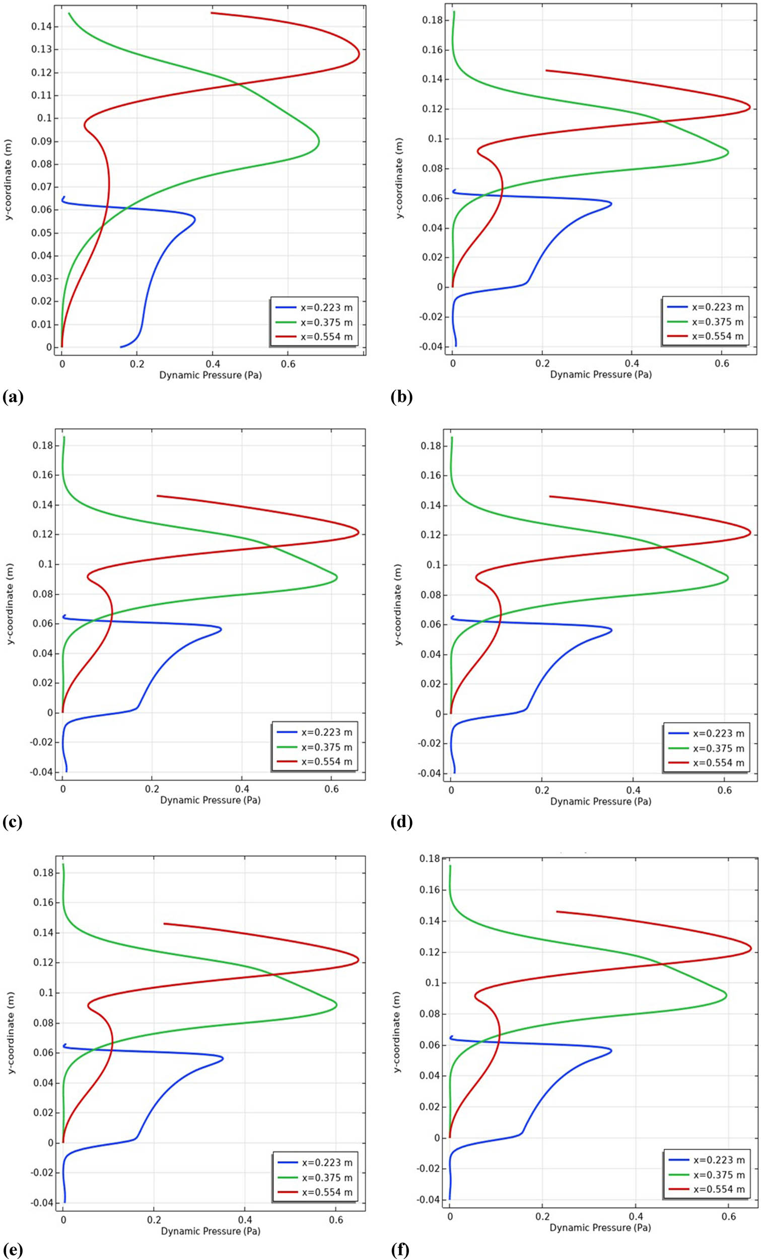
Profiles of dynamic pressure in specific stations for Re = 3,000: (a) Case 1, (b) Case 2, (c) Case 3i, (d) Case 3ii, (e) Case 3iii, and (f) Case 4.
When there are only fins present, the maximum dynamic pressure, as shown in Figure 6, is about 1.02 Pa. When grooves are present, the local dynamic pressure at these locations will become smaller to push down the entire channel pressure. As, for example, in the case of rectangular grooves, with b/c = 1, the pressure drops to 0.907 Pa. The reduction in pressure further decreases with b/c and is at about 0.878 Pa for the last value in the triangular groove, a reduction of about 13.92% from the no-groove case of 1.02 Pa.
Thus, the dynamic pressure distribution in the channel is greatly modified by obstacles and grooves. These groove structures clearly reduce the dynamic pressure, with the triangular groove offering the highest percentage reduction. The three high-pressure regions clearly show that these areas are of significantly higher pressure due to the influence of geometrical and positional features of obstacles.
Streamlines for the same Re number 3,000, in Figure 8, demonstrate how the fin geometry modifies the flow structure among all the considered cases. Indeed, the (+) and flat fins induce significant flow dynamics, where the physics of the flow varies with each different fin geometry. Since uniform axial velocity is enforced at the inlet, the flow there is uniform. This uniformity extends up to where the flow encounters the fins. In all of the cases studied, the flows were normal at locations opposite the fins, where high dynamic pressure prevails.

Streamlines depicting channel flow patterns for Re = 3,000: (a) Case 1, (b) Case 2, (c) Case 3i, (d) Case 3ii, (e) Case 3iii, and (f) Case 4.
The first fin (+) acts to disturb the flow and create an asymmetrical structure around itself. Observe how there are recirculation cells that form around all four sides of this fin. More importantly, though, there is a large recirculation zone to the right of the fin and extending far beyond the vortices that are immediately around the fin. This large vortex is due to the separation of the main flow around the obstruction caused by the fin.
This first obstacle bends the main flow toward the second fin (flat). The flow, after crossing the second fin, gets deflected upward toward the exit near the upper wall. The recirculation zone formed behind this second fin is huge in size and extends to the exit of the channel. This height of the recirculation is equal to that of the flat fin; the length of the recirculation goes to the exit of the channel. It was directly related to the existence and arrangement of the fins that created this unique flow structure.
Adding grooves to this channel gave even more complexity to the flow structure. These grooves promote more recirculation due to the low pressure inside them, which makes a flow pattern far more complicated and complex. Added recirculations and modifications in the path of flow were present.
In summary, the fins introduce large changes in the flow behavior; new recirculation regions are created, and the main flow is streamed through the channel in certain patterns. The grooves add more complexity because the low-pressure area between grooves enhances the generation of recirculations, leading to a much complex flow structure.
The velocity vector field, for different types of fins and grooves, as depicted in Figure 9, presents the complexity of airflow structures at a Re number of 3,000. In general, there is considerable influence on the flow dynamics due to the presence of fins, such as “+”-shaped and flat ones. If grooves come in various configurations, the flow behavior gets even more intricate. The design of the velocity vector field brings out two major types of flows:
Direct flow: This is the primary flow with high velocity and dynamic pressure. The flow crosses the first gap with high values of both velocity and dynamic pressure, and continues into the second gap around the upper wall all the way to the exit. It is the dominant and most important flow in regard to the general airflow of the system.
Reverse flow (recirculation zones): The recirculation zones occur on the fourth side of the “+” fin, downstream of the same fin, and also behind the second fin. These are because of flow separation at the fin ends with corresponding pressure drops. All these zones of recirculation have different dimensions, but the strongest one appears behind the flat fin. Herein, the height of the recirculation is of the same order as the fin height, and the length is from its rear to the exit.
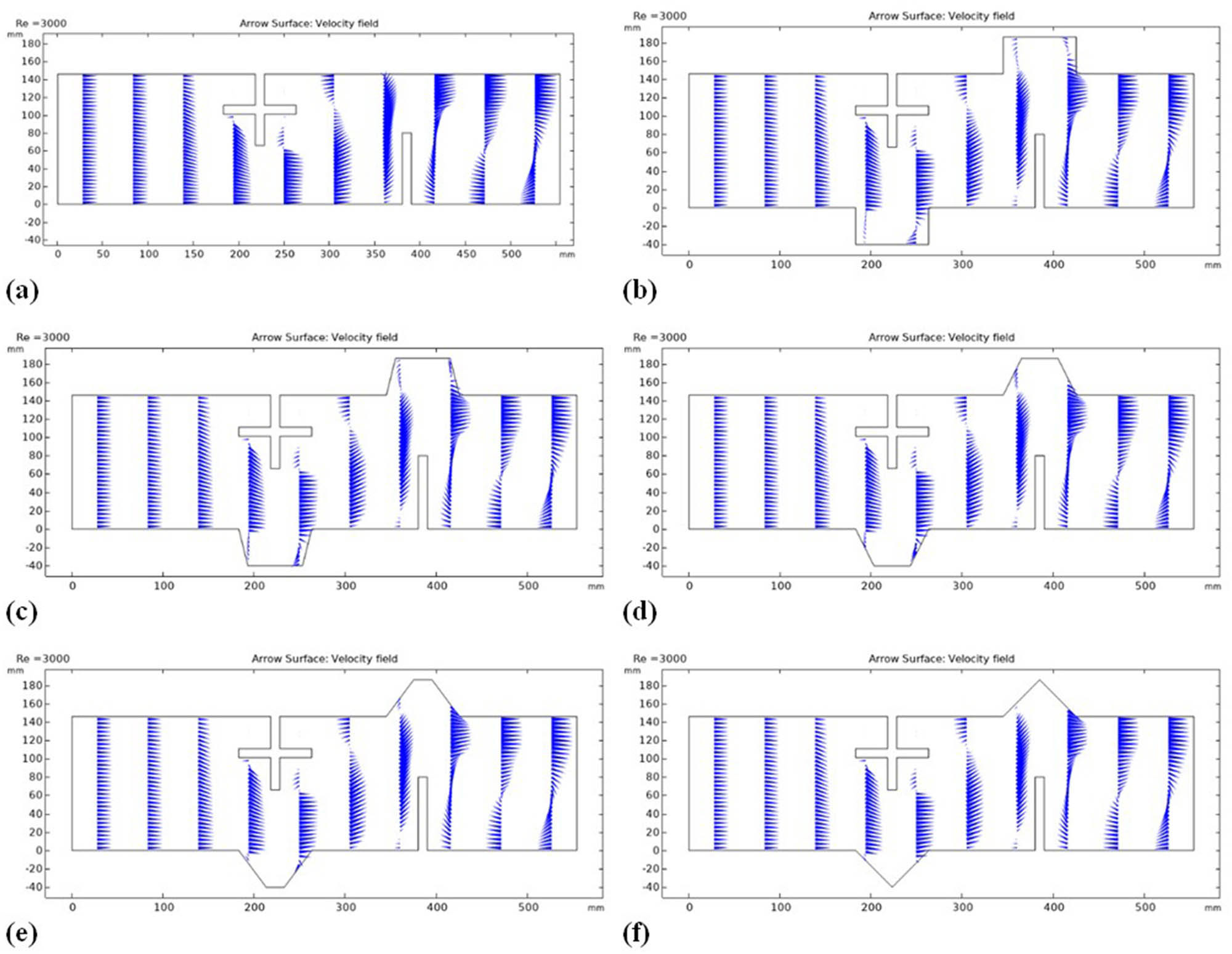
Velocity vector field illustrating flow direction for Re = 3,000: (a) Case 1, (b) Case 2, (c) Case 3i, (d) Case 3ii, (e) Case 3iii, and (f) Case 4.
Introducing grooves creates additional recirculation zones, each groove harboring its recirculation region. The size of the recirculation zones decreases as the ratio b/c reduces from 1 to 0. Rectangular grooves create larger recirculation cells, while triangular grooves create smaller ones.
The above observations represent the strong influence that geometrical parameters of fins and grooves have on the characteristics of flow, such as enhancement and hindrance of direct flow and an increase in different recirculation zones. Indeed, such an understanding is necessary in view of the optimization of fin/groove geometries for effectively improving aerodynamic performance and for suitably controlling pressure drops.
Figure 10 compares the averaged velocity contours, whereas various configurations are compared at the same Re number of 3,000. The presence of fins exhibits clear flow deceleration before the frontal areas of the fins and acceleration through the opposing areas via the gaps. The mean velocity obtained was 1.27 m/s, approximately 4.88 times the inlet velocity of 0.26 m/s. Such a large increment reflects the huge impact of fins to strongly accelerate the flow through gaps, while it has a decelerating effect in front of the fins.
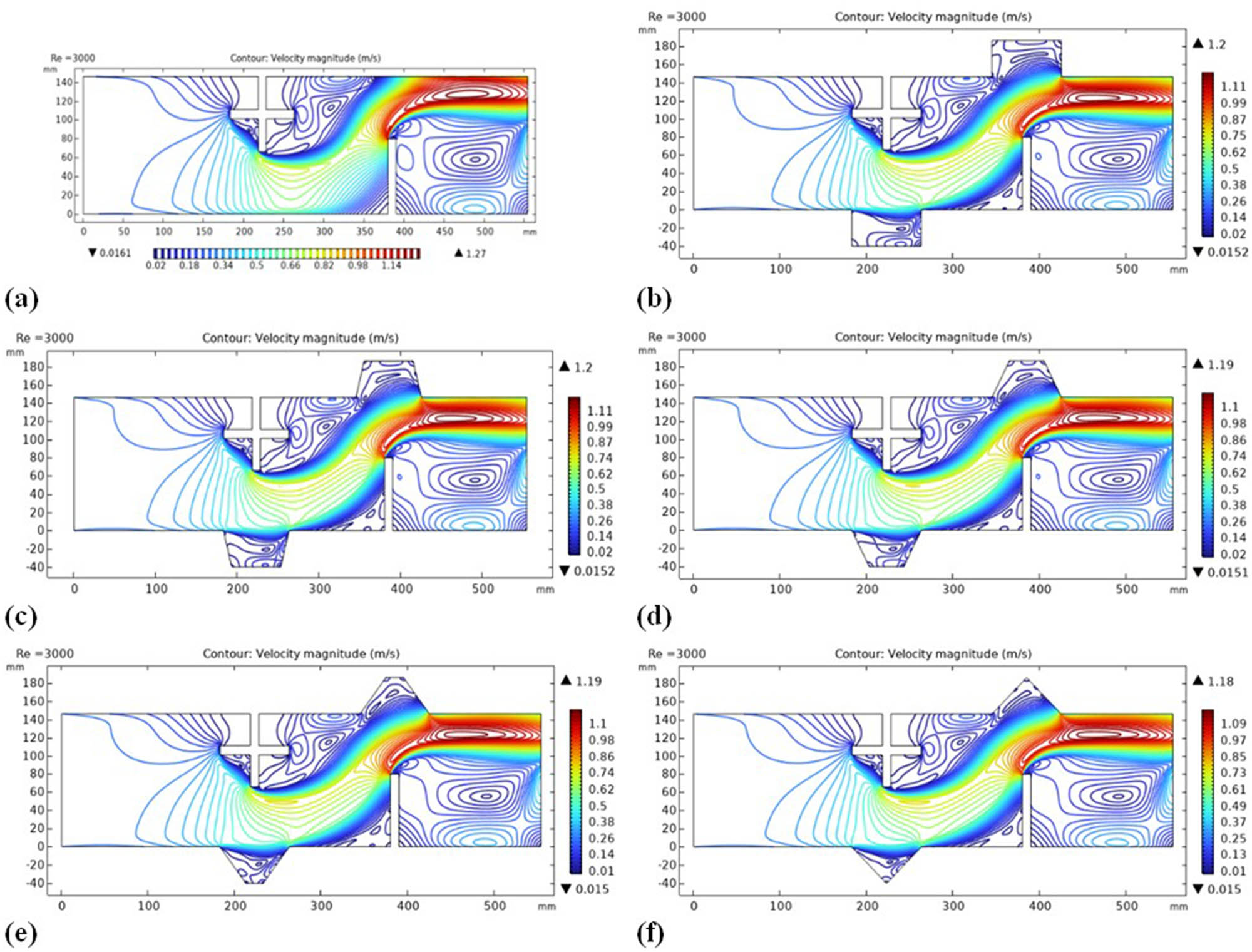
Average velocity contours along the channel length for Re = 3,000: (a) Case 1, (b) Case 2, (c) Case 3i, (d) Case 3ii, (e) Case 3iii, and (f) Case 4.
On the contrary, the addition of grooves in the system causes the velocity to drop noticeably in all the proposed cases. This results from the development of the recirculation cells, which take place as a result of the pressure drops within the grooves. More precisely, for both Case 2 and Case 3i, the average velocity decreased to 1.2 m/s, which is a reduction of about 5.5% from the finned case, which had an average of 1.27 m/s. This was further reduced to 1.19 m/s for Cases 3ii and 3iii, showing about a 6.3% reduction.
The minimum average velocity for the Case 4 triangular grooves was 1.18 m/s, which is a decline of about 7.1% from that of the first finned case. Such a trend would suggest that the groove geometry has an incrementing effect on the flow deceleration, in such a way that the case of a triangular groove would have the most pronounced effect.
Thus, grooves create a regular loss in the average velocity because of the recirculation zones formed and the accompanying pressure drops. Such behavior is in sharp contrast with the behavior of fins, where such accelerating and decelerating effects are strictly localized. The different geometries of grooves further indicate that flow characteristics are sensitive to geometric modifications; hence, the geometry of the groove configuration has to play an important role in the fluid dynamical optimization of the system.
Figure 11 shows the different velocity profiles along the x-direction between grooved and ungrooved channels. Several cases were tried in order to study/analyze the effect of grooves on the flow characteristics inside these channels.

Distribution patterns of x-velocity components in the channel for multiple configurations: (a) Case 1, (b) Case 2, (c) Case 3i, (d) Case 3ii, (e) Case 3iii, and (f) Case 4, Re = 3,000.
In the ungrooved channel, the velocity profile clearly shows the distinct low-velocity zones on both sides of every fin, which extend upstream and downstream. These zones are marked by recirculation zones, evidenced by negative values of the velocity. For instance, in Figure 12, at x = 0.285 m and x = 0.525 m, recirculation cells are obtained. These kinds of recirculation cells disturb the smooth flow, which may affect HT and pressure drop in the channel.

Axial velocity development behind the fins at Re = 3,000: (a) Case 1, (b) Case 2, (c) Case 3i, (d) Case 3ii, (e) Case 3iii, and (f) Case 4, Re = 3,000.
Further, at locations such as x = 0.223 m and x = 0.375 m shown in Figure 13, these recirculation zones are still more intensified within the groove regions. Between the bottom of the first fin (+) and the facing wall, a sharp increase in the x-velocity may be noticed. This can be viewed from Figure 13 at the location x = 0.223 m, where the increase in the above velocity has turned out to be considerably high. Similarly, there is a sharp velocity increase between the end of the flat fin and the opposite wall, especially at x = 0.375 m.

Evaluation of axial velocity through gaps, grooves, and at the exit for Re = 3,000: (a) Case 1, (b) Case 2, (c) Case 3i, (d) Case 3ii, (e) Case 3iii, and (f) Case 4.
The velocity peaks in the area downstream of the latter fin then extends up to the upper wall and toward the channel exit (see, for example, this investigated station, at x = 0.554 m, in Figure 13); the x-velocity reaches a maximum magnitude of 1.29 m/s, which is indicative of a well-developed flow regime as the fluid approaches the channel outlet. Such a peak velocity area may attest to efficient fluid acceleration past the fins and thus a well-achieved convective HT in this part of the channel.
The introduction of grooves changes the velocity profiles slightly. The x-velocity is more important since in grooved scenarios, it assumes lower values, thus reflecting changes in the flow dynamics. For example, the first grooved case decreased to 1.22 m/s in comparison to 1.29 m/s for the ungrooved case. This decrease of nearly 6% continues into other groove geometries, with the velocities hovering at approximately 1.21 m/s.
The developed y-velocity distribution patterns, in Figure 14 at Re = 3,000 variation, both represent negative and positive y-velocity values. It should be noticed that all negative y-velocity values occurred at the three edges of the fin (+). These negative y-velocity values expose a flow with a downward direction, hence indicating that the first fin channels the fluid effectively enough to flow downward through the first gap. In contrast, the positive y-velocity values are concentrated only at the leading edge of the second fin, where flow is directed upward through the second gap. This contrasting pattern underlines the effect of fin geometry on flow directions, a truly complex flow field with upward and downward alternating flows. While for the ungrooved channel, the average y-velocity was 1.16 m/s, with grooves, this velocity distribution changes significantly. The grooves dampen the y-component velocity. It is pretty clear that with the reduction in the ratio b/c from 1 to 0, a related decrease in y-velocity, which quantifies the influence of grooves in modulating the flow dynamics, is observed.

y-velocity patterns in finned channels with and without grooves for Re = 3,000: (a) Case 1, (b) Case 2, (c) Case 3i, (d) Case 3ii, (e) Case 3iii, and (f) Case 4, Re = 3,000.
The actual comparison of the effect between grooved and ungrooved channels can be analyzed through a percentage difference for the y-velocity. This will illustrate how each groove ratio, b/c, affects the flow dynamics. For example, the baseline in this experiment is the ungrooved channel, with a y-velocity of 1.16 m/s, and can be notably changed by introducing grooves. Starting with the grooved channel of a b/c of 1, one obtains a y-velocity of 0.995 m/s, which constitutes a reduction of 14.22% compared to the ungrooved case. Further reduction of the b/c ratio to 0.75 reduces the y-velocity even further to 0.985 m/s, a reduction of 15.09%. The pattern holds constant as the b/c ratio continues to decrease: at 0.5, the y-velocity decreases to 0.981 m/s, hence a 15.43% reduction; at 0.25, the y-velocity decreases to 0.97 m/s, thereby providing a reduction of 16.38%; finally, at 0, it is 0.969 m/s, thus giving a reduction of 16.47%.
It is observed that with a decrease in the b/c ratio, there is a trend of decrease in y-velocity. This may be because grooves have a tendency to enhance flow resistance and turbulence. The grooves disturb the streamline flow, leading to energy losses that reduce the general velocity of flow. Such a response indicates the critical role of groove geometry in shaping the profile of velocity and, consequently, the overall fluid dynamics of the channel.
The complicated interaction of channel geometry and flow characteristics becomes evident in the observed patterns of the y-velocity series. Thus, the flow agitated downward by the first fin and upward by the second fin supports a dynamic and alternating flow field. Furthermore, this flow is modulated by grooves that will reduce the y-velocity while enhancing mixing and HT.
Temperature contours of ungrooved and grooved channels are shown in Figure 15 for different geometries of fin and groove for the same flow rate, fixed as Re = 3,000. The primary flow of low-temperature fluid can be observed through the first gap at x = 0.223 m and the second gap at x = 0.375 m, and thereafter, is discharged from the upper part of the channel at x = 0.554 m. These profiles, as represented in Figure 16, point out regions of high-velocity and dynamic pressure values.

Temperature patterns in finned channels with and without grooves for Re = 3,000: (a) Case 1, (b) Case 2, (c) Case 3i, (d) Case 3ii, (e) Case 3iii, and (f) Case 4, Re = 3,000.

Detailed analysis of temperature across gaps, grooves, and exit at Re = 3,000: (a) Case 1, (b) Case 2, (c) Case 3i, (d) Case 3ii, (e) Case 3iii, and (f) Case 4, Re = 3,000.
The recirculation regions, represented by reverse flow on the rear of both fins, can also be seen at relatively high temperatures, as shown at x = 0.285 m beyond the first fin and also at x = 0.525 m beyond the second fin. The temperature profiles associated with this region are further elaborated, as shown in Figure 17. From the figure, it is evident that the maximum temperature developed in these regions without a groove over the channel is close to 62.2°C.

Temperature development downstream of fins at Re = 3,000: (a) Case 1, (b) Case 2, (c) Case 3i, (d) Case 3ii, (e) Case 3iii, and (f) Case 4, Re = 3,000.
The grooves tended to increase it considerably. Specific examples are shown where rectangular grooves raise the temperature to 74.1°C, representing an increase of around 19.13%. Trapezoidal grooves increase the temperature further: increases to 74.4°C for b/c = 0.75, to 74.8°C for b/c = 0.50, and to 75.6°C for b/c = 0.25, corresponding, respectively, to increases around 19.61, 20.25, and 21.54% over the base value. The triangular grooves at b/c = 0 increase the temperature to 75.1°C. Compared with the ungrooved channel, this gives an enhanced growth of approximately 20.73%.
These results provide evidence that the addition of grooves in the channel significantly alters flow dynamics and, more importantly, improves thermal performance due to increased maximum temperature within the channel. Full temperature profiles across different grooved channels represent the efficiency of geometric modifications to optimize thermal management.
In particular, the rectangular grooves increased the temperature by 11.9°C, trapezoidal grooves with b/c ratios of 0.75, 0.50, and 0.25 increased the temperatures to 12.2, 12.6, and 13.4°C, respectively, and triangular grooves further raised it by 12.9°C. From these fundamental improvements, it can be expected that the geometry is one of the most important factors affecting the performance of the groove in enhancing local HT. Consequently, the increase in temperature is due to the grooves’ effect of improved mixing and disruption of flow that enhances the efficiency of the HT process.
We have analyzed the average temperature at the channel exit for the various configurations in order to compare their heat performances (Table 4). The ungrooved channel had lower performance, with an average outlet temperature of 36.79°C. The introduction of the rectangular grooves raised this temperature to 38.38°C, which is about a 4.32% improvement. Accordingly, trapezoidal grooves added to the average outlet temperature increase of about 38.33–38.41°C or approximately an increase of 4.18–4.40%.
Evaluation of thermal performance in ungrooved and grooved channels, T inlet = 27°C
| Ungrooved and grooved cases | |||||
|---|---|---|---|---|---|
| Case 1 | Case 2 | Case 3i | Case 3ii | Case 3iii | Case 4 |
| b / c ratio | |||||
| / | 1.00 | 0.75 | 0.50 | 0.25 | 0.00 |
| Mean outlet temperature, T out (°C) | |||||
| 36.79 | 38.38 | 38.41 | 38.37 | 38.33 | 38.24 |
| Δ T (°C) = T out – T inlet | |||||
| 9.79 | 11.38 | 11.41 | 11.37 | 11.33 | 11.24 |
Again, the trapezoidal shapes gave the maximum temperature to case 3i of 38.41°C with a b/c ratio of 0.75, which is slightly higher than the case of 3ii by about 0.10% and case 3iii by about 0.21%. On the contrary, the average temperature because of triangular grooves was 38.24°C, which is an enhancement of 3.94% over the ungrooved channel.
Triangle grooves gave some enhancement, but were the poorest performer out of the grooved cases. The temperature increase for the case of rectangular grooves is also about 0.36% higher than triangular grooves, while trapezoidal grooves manifested further enhancements of 0.23–0.44% over triangular grooves.
From the trapezoidal grooved configurations, the groove with a b/c value of 0.75 represented case 3i, which indeed gave the best thermal performance among all cases studied in terms of its efficacy in enhancing the average outlet temperature. This comparative study hence established that groove geometry and configuration are the most critical elements in the optimization of thermal efficiency, while among the trapezoidal grooves, a b/c value of 0.75 provides the most enhanced levels.
Temperature differences between the outlet and inlet for all channel designs were studied to find the best case for various grooved channel geometries. The temperature difference ΔT obtained for a non-grooved channel (Case 1), a channel with rectangular groove of b/c = 1, and three channels with trapezoidal grooves of b/c = 0.75, b/c = 0.5, and b/c = 0.25, and channel with triangular grooves of b/c = 0 is represented by the data portrayed.
Accordingly, the ΔT values are as follows. Case 1: 9.79°C, Case 2: 11.38°C, Case 3i: 11.41°C, Case 3ii: 11.37°C, Case 3iii: 11.33°C, and Case 4: 11.24°C. Thus, the highest thermal performance of Case 3i is given by ΔT = 11.41°C.
To give a clear quantification of the enhancements with respect to the ungrooved channel, Case 1, we have calculated the percentage enhancement in ΔT for each configuration. Thus, Case 2 (rectangular grooves) yields an enhancement of 16.23%, whereas Case 3i (trapezoidal grooves, b/c = 0.75) yields an enhancement of 16.54%, which is thus the optimal geometry. Case 3ii yields an enhancement of 16.14%, Case 3iii gives an enhancement of 15.75%, and Case 4 (triangular grooves) yields an enhancement of 14.81%. Among them, Case 3i with trapezoidal grooves at a b/c ratio of 0.75 is the best, which provides the highest ΔT compared to the other grooved or ungrooved channels.
This part develops the contribution of the size of the first fin, the one in the (+) shape, on thermal performance in a trapezoidal grooved channel. With h = 0.08 m and keeping the second fin flat at h, the first fin is increased through values of 0.25, 0.50, 0.75, 1.00, 1.25, and 1.50 h. The Reynolds number has been maintained as Re = 3,000, whereas the best groove optimum case of b/c = 0.75 was used for this study. The temperature fields for all different fin sizes were scrutinized to select the most effective configuration based on HT enhancement.
Figure 18 presents the temperature fields for all possible fin sizes. With the increase in size of the (+) fin, the fluid temperature within the channel increases gradually due to larger HT surfaces provided by larger fins. From the temperature distribution, one can identify that for fin sizes in the range of 0.25–1.00 h, the enhancement of fluid temperature will be relatively poor. Whereas for larger fin sizes, 1.25 and 1.50 h, the temperature profile improved drastically, thereby enhancing the HT process.

Impact of first fin size (+) on the temperature fields (b/c = 0.75) for Re = 3,000: (a) 0.25 h, (b) 0.50 h, (c) 0.75 h, (d) 1.00 h, (e) 1.25 h, and (f) 1.50 h.
For larger fin sizes, the high temperature regions are primarily located downstream of the first fin, along the second fin, and in the upper and lower grooves. This temperature distribution suggests that larger fins create stronger convective HT.
The mean outlet temperatures (T out) for several “+” fin sizes are listed in Table 5. From the increase of the “+” fin size, the average value of T out increases, indicating that the thermal performance is proportional to the “+” fin size. For the smallest fin size, 0.25 h, the average outlet temperature was 33.83°C, while it reached 46.35°C for the largest fin size of 1.50 h, a notable improvement.
Thermal performance analysis of the fin size ( +) in a trapezoidal grooved channel (b/c = 0.75)
| Fin size (+) | |||||
| 0.25 h | 0.50 h | 0.75 h | 1.00 h | 1.25 h | 1.50 h |
| Mean outlet temperature, T out (°C) | |||||
| 33.83 | 34.62 | 36.00 | 38.41 | 42.03 | 46.35 |
| Δ T (°C) = T out – T inlet | |||||
| 6.83 | 7.62 | 9.00 | 11.41 | 15.03 | 19.35 |
Further clarification is obtained from the temperature difference, ΔT, which increased from 6.83°C for the smallest “+” fin size to 19.35°C for the largest “+” fin size. This significant increase in the temperature difference further indicates how large the dimensions of the “+” fins serve to enhance thermal performance effectively. From the comparison of the thermal performance of all these cases, the “+” fin size of 1.50 h was found to be the optimal configuration. It gives the highest mean outlet temperature of 46.35°C and the largest temperature difference ΔT = 19.35°C. It maximizes the HT efficiency, showing a 183.30% enhancement in ΔT over that from the smallest size.
With a view to further optimizing the performance of this heat exchanger channel, we now focus on the analysis regarding the effect of the size variation of the flat fin, in contrast to the previously studied (+) fin. The height of the (+) fin is kept constant at h, while the height variation in the flat fin increases from 0.25 to 1.50 h. The detailed work is given below for thorough examination of the fluid temperature field, shown in Figure 19, investigation of the average outlet temperature and the temperature difference depicted in Table 6.

Effect of the second fin’s dimensions on temperature distributions (b/c = 0.75) at Re = 3,000: (a) 0.25 h, (b) 0.50 h, (c) 0.75 h, (d) 1.00 h, (e) 1.25 h, and (f) 1.50 h.
Thermal performance comparison for different second fin sizes in a trapezoidal grooved channel (b/c = 0.75)
| Fin size (flat) | |||||
| 0.25 h | 0.50 h | 0.75 h | 1.00 h | 1.25 h | 1.50 h |
| Mean outlet temperature, T out (°C) | |||||
| 34.35 | 35.12 | 36.75 | 38.41 | 40.18 | 40.47 |
| Δ T (°C) = T out – T inlet | |||||
| 7.35 | 8.12 | 9.75 | 11.41 | 13.18 | 13.47 |
In general, the zones of channel temperature are the highest near the surfaces heated. As expected, this temperature distribution improves significantly inside the channel, with an increase in the HT surface area achieved by increasing the size of the flat fin. This effect is more pronounced for the recirculation zones, where a greater area increases the heat spread. The temperature of the fluid also increases significantly at the exit compared to the inlet, proving that heat exchange in this configuration is more effective. It shows the probable gain that may arise from optimization of the fin geometry to achieve better thermal performance for the heat exchanger channels.
As can be seen from Table 6, the data clearly illustrate the thermal performance variation with each of the flat fin sizes. For example, for a 0.25 h flat fin size, T out is 34.35°C, with a ΔT of 7.35°C. Correspondingly, by increasing the flat fin size to 0.50 h, T out is estimated to be 35.12°C and ΔT is estimated to be 8.12°C, which indicates an increase of about 2.24% in the T out and about 10.47% in ΔT compared with a 0.25 h flat fin size. A further increase in size to 0.75 h further increases the T out to 36.75°C and ΔT to 9.75°C, recording a 4.64% increase in T out and a 20.07% increase in ΔT over the flat fin size of 0.50 h. For a flat fin size of 1.00 h, T out is 38.41°C and ΔT is 11.41°C, an increase of 4.51 °C and 17.02% over the 0.75 h flat fin size. Correspondingly, for the 1.25 h flat fin size, T out increases to 40.18°C with a ΔT of 13.18°C, indicating an increase of 4.60% in T out and 15.51% in ΔT compared to the 1.00 h flat fin size. T out becomes the highest at 40.47°C, and ΔT is at 13.47°C, while T out increased by 0.72%, and ΔT by 2.20% for the largest flat fin size at 1.50 h from the 1.25 h flat fin size.
Comparing the performance of all flat fin sizes, it can be realized that an increase in flat fin heights will result in higher HT performances; this is manifested in progressive average outlet temperature and temperature differences. Most improvements are, however, between the smaller size of flat fins, especially from 0.25 to 0.75 h. Beyond a 1.00 h flat fin size, the rate of improvement begins to diminish, and the 1.50 h flat fin has very limited improvement over the 1.25 h flat fin.
When evaluating the integrated impact of fin size on thermal performance, fin sizes ranged from 0.25 to 1.50 h. From the temperature contour plots shown in Figure 20 and in Table 7, we can find the average temperatures for variations mentioned in this study at the outlet. In the present work, we used a trapezoidal groove with a b/c ratio of 0.75, keeping a fixed flow rate of 3,000. From the results presented, it is possible to identify a certain trend: the increase of the fin dimension promotes an increase of the HT surface area, raising the fluid temperature notably. This effect is more dramatic for large dimensions of fins, showing extended temperature increases along the back sides of the fins.

Temperature fields affected by “+” and flat fin sizes (b/c = 0.75) at Re = 3,000: (a) 0.25 h, (b) 0.50 h, (c) 0.75 h, (d) 1.00 h, (e) 1.25 h, and (f) 1.50 h.
An examination of the combined “+” and flat fin sizes’ thermal performance in a trapezoidal grooved channel (b/c = 0.75)
| Fin size | |||||
| 0.25 h | 0.50 h | 0.75 h | 1.00 h | 1.25 h | 1.50 h |
| Mean outlet temperature, T out (°C) | |||||
| 29.32 | 31.11 | 34.28 | 38.41 | 44.06 | 51.17 |
| Δ T (°C) = T out – T inlet | |||||
| 2.32 | 4.11 | 7.28 | 11.41 | 17.06 | 24.17 |
Table 7 gives a detailed analysis of thermal performance using different sizes of fins in the trapezoidal grooved channel. It can be realized that the average value of outlet temperature, T out, remarkably increases from 29.32°C for 0.25 h to up to 51.17°C for 1.50 h. It can be noticed that ΔT has significantly increased between the outlet and inlet temperatures, ranging from 2.32°C for 0.25 h to 24.17°C for 1.50 h. The large increase in ΔT indicates higher HT capability for the larger fin size. Hence, the fin size that would give an optimum thermal performance based on temperature increase and efficiency is 1.50 h. This size provides the largest surface area, enhancing the HT and providing the highest recorded increase in temperature with an overall improved thermal performance.
This optimum setup has an astonishing improvement in performance compared to other setups. Specifically, a single first fin in the shape of a plus (+) at 1.50 h gave a temperature difference of 19.35°C, which showed a significant enhancement but not as high as for both fins in combination. The single second fin in flat shape at 1.50 h gave a temperature difference of 13.47°C. Comparing these respective optimum cases to one another, the combined fins configuration is significantly increased by 24.90% over the first fin alone and by 79.43% over the second fin alone. Thus, their combination at 1.50 h performs not only better than both single-fin configurations but also manifests the synergistic effect of using both-fin types together for the best thermal performance.
4 Conclusions
This numerical research using finite elements has compared comprehensively the hydrothermal performance of turbulent flow within rectangular channels and various groove and fin geometries. The work was conducted in two phases: the first comparison was between the impact of shapes of the grooves, while the second compared the impact of the height of the fin in two different categories of fins (“+” and flat).
Phase I, in which the introduction of grooves significantly improved thermal performance, indicated that all cases with a trapezoidal groove were considerably better than the ungrooved channel. Among all cases, Case 3i, with b/c = 0.75, indicated the best performance by increasing the mean outlet temperature by 38.41 °C, an increase of approximately 16.54% in ΔT.
In Phase II, the variation of fin height with the optimum groove configuration showed taller fins resulting in more HT in all cases. Highest augmentation was achieved when the “+” and flat fins were both 1.50 h in height, with an average outlet temperature of 51.17°C and ΔT of 24.17°C, a 146.88% augmentation over the reference ungrooved channel and 941.81% compared to the minimum fin setup. This definitively illustrates the intense synergy between groove shape and fin height.
4.1 Application
Such results are of the most significance in the optimization of thermal efficiency of solar HEs, especially in applications with compact, high-performance designs required, such as solar collectors, electronics cooling, or compact thermal storage devices.
4.2 Future research perspectives
Further research may explore transient flow characteristics, multiple turbulence models to enhance accuracy, and the use of nanofluids to further enhance thermal conductivity. Experimental validation and extension to non-rectangular or curved geometries would also provide greater usefulness in actual solar thermal applications.
Acknowledgments
The authors acknowledge Princess Nourah bint Abdulrahman University Researchers Supporting Project number (PNURSP2025R826), Princess Nourah bint Abdulrahman University, Riyadh, Saudi Arabia.
-
Funding information: This study was funded by Princess Nourah bint Abdulrahman University Researchers Supporting Project number (PNURSP2025R826), Princess Nourah bint Abdulrahman University, Riyadh, Saudi Arabia.
-
Author contributions: Younes Menni: conceptualization (equal); investigation (equal); writing – original draft (equal); and writing – review and editing (equal). Noureddine Kaid: methodology (equal); software (equal); writing – original draft (equal); and writing – review and editing (equal). Samia Larguech: Data curation (equal); formal analysis (equal); writing – original draft (equal); and writing – review and editing (equal). Badr M. Alshammari: methodology (equal); validation (equal); writing – original draft (equal); writing – review and editing (equal). Lioua Kolsi: resources (equal); software (equal); writing – original draft (equal); and writing – review and editing (equal). All authors have accepted responsibility for the entire content of this manuscript and approved its submission.
-
Conflict of interest: The authors state no conflict of interest.
-
Data availability statement: The datasets generated and/or analyzed during the current study are available from the corresponding author on reasonable request.
References
[1] Singh S, Dhiman P. Thermal and thermohydraulic efficiency of recyclic-type double-pass solar air heaters with fins and baffles. Heat Transf Eng. 2016;37(15):1302–17. 10.1080/01457632.2015.1119619.Search in Google Scholar
[2] Eiamsa-Ard S, Phila A, Thianpong C, Chuwattanakul V, Maruyama N, Hirota M. Evaluation of heat transfer performance of a channel mounted with square-wing perforated V-type baffles. Exp Heat Transf. 2024;38(4):378–404. 10.1080/08916152.2024.2341743.Search in Google Scholar
[3] Esmaeili Z, Rashidi S. Entropy production analysis for nanofluid flow through a channel with perforated transverse twisted-baffles. Energy Sources Part A: Recovery Util Environ Eff. 2022;1–20. 10.1080/15567036.2022.2041131.Search in Google Scholar
[4] Lopez JR, Anand NK, Fletcher LS. Heat transfer in a three-dimensional channel with baffles. Numer Heat Transf Part A Appl. 1996;30(2):189–205. 10.1080/10407789608913835.Search in Google Scholar
[5] Santos NB, de Lemos MJ. Flow and heat transfer in a parallel-plate channel with porous and solid baffles. Numer Heat Transf Part A: Appl. 2006;49(5):471–94. 10.1080/10407780500325001.Search in Google Scholar
[6] Da Silva Miranda BM, Anand NK. Convective heat transfer in a channel with porous baffles. Numer Heat Transf Part A: Appl. 2004;46(5):425–52. 10.1080/10407780490478515.Search in Google Scholar
[7] Yang YT, Tsai KT, Tang HW, Chung SE. Numerical simulations and optimization of porous pin fins in a rectangular channel. Numer Heat Transf Part A: Appl. 2016;70(7):791–808. 10.1080/10407782.2016.1214479.Search in Google Scholar
[8] Kheradmand-Laleh A, Hossainpour S, Keyhani-Asl A, Vatanparast MA. Effect of utilizing staggered semi-porous fins on channel flow heat transfer enhancement. Heat Transf Eng. 2023;44(14):1244–61. 10.1080/01457632.2022.2127047.Search in Google Scholar
[9] Venkatesh G, Meenakshi Reddy R. Experimental and numerical investigation of flow and heat transfer characteristics of teardrop and circular pin fins in a wedge channel. Exp Heat Transf. 2024;1–20. 10.1080/08916152.2024.2392808.Search in Google Scholar
[10] Perão LH, Zdanski PSB, Vaz Jr M. Conjugate heat transfer in channels with heat-conducting inclined fins. Numer Heat Transf Part A: Appl. 2018;73(2):75–93. 10.1080/10407782.2017.1420309.Search in Google Scholar
[11] Aouissi Z, Chabane F. Numerical and experimental study of thermal efficiency of the transversal rectangular baffles with incline angle inside of solar air collector. Energy Sources Part A: Recovery Util Environ Eff. 2022;44(4):8921–42. 10.1080/15567036.2022.2128474.Search in Google Scholar
[12] Chamoli S, Thakur NS. Thermal behavior in rectangular channel duct fitted with v-shaped perforated baffles. Heat Transf Eng. 2015;36(5):471–9. 10.1080/01457632.2014.935218.Search in Google Scholar
[13] Chabane F, Grira F, Moummi N, Brima A. Experimental study of a solar air heater by adding an arrangement of transverse rectangular baffles perpendicular to the air stream. Int J Green Energy. 2019;16(14):1264–77. 10.1080/15435075.2019.1671401.Search in Google Scholar
[14] Jain SK, Misra R, Kumar A, Agrawal GD. Thermal performance investigation of a solar air heater having discrete V-shaped perforated baffles. Int J Ambient Energy. 2022;43(1):243–51. 10.1080/01430750.2019.1636874.Search in Google Scholar
[15] Mukilarasan N, Karthikeyan R, Ramalingam S, Dillikannan D, Ravikumar J, Sampath S, et al. Influence of baffles in heat transfer fluid characteristics using CFD evaluation. Int J Ambient Energy. 2022;43(1):7088–100. 10.1080/01430750.2022.2063175.Search in Google Scholar
[16] Henniche R, Korichi A. Heat transfer enhancement in self-sustained oscillatory flow in a staggered baffled vertical channel under the buoyancy effect. Numer Heat Transfer Part A: Appl. 2017;71(12):1189–204.10.1080/10407782.2017.1353370Search in Google Scholar
[17] Wang Q, Chen G, Chen Q, Zeng M. Review of improvements on shell-and-tube heat exchangers with helical baffles. Heat Transf Eng. 2010;31(10):836–53. 10.1080/01457630903547602.Search in Google Scholar
[18] Sharma S, Das RK, Kulkarni K. Parametric optimization of solar air heater having sine wave baffles as turbulators. Exp Heat Transf. 2024;37(2):182–207. 10.1080/08916152.2022.2108525.Search in Google Scholar
[19] Naqvi SMA, Wang Q. Performance enhancement of shell–tube heat exchanger by clamping anti-vibration baffles with porous media involvement. Heat Transf Eng. 2021;42(18):1523–38. 10.1080/01457632.2020.1807098.Search in Google Scholar
[20] Joye DD, Côté AS. Heat transfer enhancement in annular channels with helical and longitudinal fins. Heat Transf Eng. 1995;16(2):29–34. 10.1080/01457639508939850.Search in Google Scholar
[21] Thomas Renald CJ, Somasundaram P, Matheswaran MM, Gnanasekaran N. Analytical investigation on thermo hydraulic performance augmentation of triangular duct solar air heater integrated with wavy fins. Int J Green Energy. 2023;20(5):544–54. 10.1080/15435075.2022.2111215.Search in Google Scholar
[22] Michael Joseph Stalin P, Rao PN, Palaniappan M, Kumar PM, Udhayakumar K. Effective thermal performance assessment for prismatic triangular solar air heater integrated with fins and turbulators. Numer Heat Transf Part A: Appl. 2024;1–17. 10.1080/10407782.2024.2357592.Search in Google Scholar
[23] Wang C, Zhu JG, Sang ZF. Experimental studies on thermal performance and flow resistance of heat exchangers with helical baffles. Heat Transf Eng. 2009;30(5):353–8. 10.1080/01457630802414540.Search in Google Scholar
[24] Menni Y, Chamkha AJ, Ghazvini M, Ahmadi MH, Ameur H, Issakhov A, et al. Enhancement of the turbulent convective heat transfer in channels through the baffling technique and oil/multiwalled carbon nanotube nanofluids. Numer Heat Transf Part A: Appl. 2020;79(4):311–51. 10.1080/10407782.2020.1842846.Search in Google Scholar
[25] Fourar I, Benmachiche AH. The effect of using circular fins with a V-shaped cut on the weight reduction and the overall performance of a finned tube heat exchanger. Int J Ambient Energy. 2022;43(1):7020–9. 10.1080/01430750.2022.2059005.Search in Google Scholar
[26] Sharma AK, Mahapatra PS, Manna NK, Ghosh K. Mixed convection heat transfer in a grooved channel in the presence of a baffle. Numer Heat Transf Part A: Appl. 2015;67(10):1097–118. 10.1080/10407782.2014.955359.Search in Google Scholar
[27] Yang K, Sui Y, Wang X, Feng Z. Study on flow and heat transfer characteristics in rectangular channels with lantern-shaped pin fin array: Part I-effect of sphere diameter. Numer Heat Transf Part A: Appl. 2023;86(4):813–43. 10.1080/10407782.2023.2251085.Search in Google Scholar
[28] Chabane F, Kherroubi D, Arif A, Moummi N, Brima A. Influence of the rectangular baffle on heat transfer and pressure drop in the solar collector. Energy Sources Part A: Recovery Util Environ Eff. 2020;46(1):8547–63. 10.1080/15567036.2020.1767727.Search in Google Scholar
[29] Tsay YL, Cheng JC, Chang TS. Enhancement of heat transfer from surface-mounted block heat sources in a duct with baffles. Numer Heat Transf: Part A: Appl. 2003;43(8):827–41. 10.1080/713838151.Search in Google Scholar
[30] Facas GN. Natural convection from a buried pipe with external baffles. Numer Heat Transf Part A: Appl. 1995;27(5):595–609. 10.1080/10407789508913720.Search in Google Scholar
[31] Ahmadinejad M, Soleimani A, Gerami A. Performance enhancement of a photovoltaic thermal (PVT) system with sinusoidal fins: A quasi-transient energy-exergy analysis. Int J Green Energy. 2023;20(9):978–96. 10.1080/15435075.2022.2131434.Search in Google Scholar
[32] Shaeri MR, Jen TC. Turbulent heat transfer analysis of a three-dimensional array of perforated fins due to changes in perforation sizes. Numer Heat Transf Part A: Appl. 2012;61(11):807–22. 10.1080/10407782.2012.671046.Search in Google Scholar
[33] Demartini LC, Vielmo HA, Möller SV. Numeric and experimental analysis of the turbulent flow through a channel with baffle plates. J Braz Soc Mech Sci Eng. 2004;26:153–9. 10.1590/S1678-58782004000200006.Search in Google Scholar
[34] Kedar SA, More GV, Watvisave DS, Shinde HM. A critical review on the various techniques for the thermal performance improvement of solar air heaters. Energy Sources Part A: Recovery Util Environ Eff. 2023;45(4):11819–52. 10.1080/15567036.2023.2264228.Search in Google Scholar
[35] Goel AK, Singh SN. Performance studies of a jet plate solar air heater with longitudinal fins. Int J Ambient Energy. 2019;40(2):119–27. 10.1080/01430750.2017.1372808.Search in Google Scholar
[36] Berber A, Gürdal M, Yetimoğlu M. Experimental study on the heat transfer enhancement in a rectangular channel with curved winglets. Exp Heat Transf. 2022;35(6):797–817. 10.1080/08916152.2021.1951897.Search in Google Scholar
[37] Ishaq M, Ul Haq I, Saifullah Syed K. Heat transfer enhancement in finned annulus of elliptic-circular heat exchanger. Numer Heat Transf Part A: Appl. 2023;86(6):1452–80. 10.1080/10407782.2023.2273991.Search in Google Scholar
[38] Omri M, Selimefendigil F, Besbes H, Ladhar L, Alshammari BM, Kolsi L. Analysis of MHD nanofluid forced convection and phase change process in a PCM mounted corrugated and partly elastic partitioned channel system with area expansion. J Eng Res. 2024. 10.1016/j.jer.2024.12.012.Search in Google Scholar
[39] Selimefendigil F, Benabdallah F, Ghachem K, Albalawi H, Alshammari BM, Kolsi L. Single-channel cooling system design by using perforated porous insert and modeling with POD for double conductive panel. Open Phys. 2024;22(1):20240107. 10.1515/phys-2024-0107.Search in Google Scholar
[40] Ben Said L, Kolsi L, Ben Khedher N, Alshammari F, Malekshah EH, Hussein AK. Numerical study of the fluid-structure interaction during CNT-water nanofluid mixed convection in a micro-channel equipped with elastic fins under periodic inlet velocity conditions. Exp Tech. 2023;47:7–15. 10.1007/s40799-021-00527-4.Search in Google Scholar
[41] Si W, Fu C, Tian Y, Chen J, Yuan P, Huang Z, et al. Numerical study of flow and heat transfer in the channel of panel-type radiator with semi-detached inclined trapezoidal wing vortex generators. Open Phys. 2024;22(1):20230180. 10.1515/phys-2023-0180.Search in Google Scholar
[42] Wang W, Zhang B, Cui L, Zheng H, Klemeš JJ, Wang J. Numerical study on heat transfer and flow characteristics of nanofluids in a circular tube with trapezoid ribs. Open Phys. 2021;19(1):224–33. 10.1515/phys-2021-0022.Search in Google Scholar
[43] Kumar MD, Raju CSK, Shah NA, Yook SJ, Gurram D. Support vector machine learning classification of heat transfer rate in tri-hybrid nanofluid over a 3D stretching surface with suction effects for water at 10°C and 50°C. Alex Eng J. 2025;118:556–78. 10.1016/j.aej.2025.01.061.Search in Google Scholar
[44] Kumar MD, Dharmaiah G, Yook SJ, Raju CSK, Shah NA. Deep learning approach for predicting heat transfer in water-based hybrid nanofluid thin film flow and optimization via response surface methodology. Case Stud Therm Eng. 2025;68:105930. 10.1016/j.csite.2025.105930.Search in Google Scholar
[45] Kumar MD, Raju CSK, Sajjan K, Dharmaiah G, Shah NA, Yook SJ. Deep neural network-based prediction and computational fluid dynamics analysis of convective heat transfer in dusty fluid flow over heated surface. Phys Fluids. 2025;37(2):023112. 10.1063/5.0250396.Search in Google Scholar
[46] Launder BE, Spalding DB. The numerical computation of turbulent flows. Comput Methods Appl Mech Eng. 1974;3(2):269–89. 10.1016/0045-7825(74)90029-2.Search in Google Scholar
[47] COMSOL Multiphysics® v. 5.0. www.comsol.com. Stockholm, Sweden: COMSOL AB; 2014.Search in Google Scholar
[48] Siddiqui MHK. Heat transfer augmentation in a heat exchanger tube using a baffle. Int J Heat Fluid Flow. 2007;28(2):318–28. 10.1016/j.ijheatfluidflow.2006.03.020.Search in Google Scholar
[49] Bathe KJ. Finite element method. Wiley Encycl Comput Sci Eng. 2007;1–12. 10.1002/9780470050118.ecse159.Search in Google Scholar
[50] Hinze J. Turbulence. New York: McGraw-Hill; 1975.Search in Google Scholar
[51] Sahel D, Ameur H, Benzeguir R, Kamla Y. Enhancement of heat transfer in a rectangular channel with perforated baffles. Appl Therm Eng. 2016;101:156–64. 10.1016/j.applthermaleng.2016.02.136.Search in Google Scholar
© 2025 the author(s), published by De Gruyter
This work is licensed under the Creative Commons Attribution 4.0 International License.
Articles in the same Issue
- Research Articles
- Single-step fabrication of Ag2S/poly-2-mercaptoaniline nanoribbon photocathodes for green hydrogen generation from artificial and natural red-sea water
- Abundant new interaction solutions and nonlinear dynamics for the (3+1)-dimensional Hirota–Satsuma–Ito-like equation
- A novel gold and SiO2 material based planar 5-element high HPBW end-fire antenna array for 300 GHz applications
- Explicit exact solutions and bifurcation analysis for the mZK equation with truncated M-fractional derivatives utilizing two reliable methods
- Optical and laser damage resistance: Role of periodic cylindrical surfaces
- Numerical study of flow and heat transfer in the air-side metal foam partially filled channels of panel-type radiator under forced convection
- Water-based hybrid nanofluid flow containing CNT nanoparticles over an extending surface with velocity slips, thermal convective, and zero-mass flux conditions
- Dynamical wave structures for some diffusion--reaction equations with quadratic and quartic nonlinearities
- Solving an isotropic grey matter tumour model via a heat transfer equation
- Study on the penetration protection of a fiber-reinforced composite structure with CNTs/GFP clip STF/3DKevlar
- Influence of Hall current and acoustic pressure on nanostructured DPL thermoelastic plates under ramp heating in a double-temperature model
- Applications of the Belousov–Zhabotinsky reaction–diffusion system: Analytical and numerical approaches
- AC electroosmotic flow of Maxwell fluid in a pH-regulated parallel-plate silica nanochannel
- Interpreting optical effects with relativistic transformations adopting one-way synchronization to conserve simultaneity and space–time continuity
- Modeling and analysis of quantum communication channel in airborne platforms with boundary layer effects
- Theoretical and numerical investigation of a memristor system with a piecewise memductance under fractal–fractional derivatives
- Tuning the structure and electro-optical properties of α-Cr2O3 films by heat treatment/La doping for optoelectronic applications
- High-speed multi-spectral explosion temperature measurement using golden-section accelerated Pearson correlation algorithm
- Dynamic behavior and modulation instability of the generalized coupled fractional nonlinear Helmholtz equation with cubic–quintic term
- Study on the duration of laser-induced air plasma flash near thin film surface
- Exploring the dynamics of fractional-order nonlinear dispersive wave system through homotopy technique
- The mechanism of carbon monoxide fluorescence inside a femtosecond laser-induced plasma
- Numerical solution of a nonconstant coefficient advection diffusion equation in an irregular domain and analyses of numerical dispersion and dissipation
- Numerical examination of the chemically reactive MHD flow of hybrid nanofluids over a two-dimensional stretching surface with the Cattaneo–Christov model and slip conditions
- Impacts of sinusoidal heat flux and embraced heated rectangular cavity on natural convection within a square enclosure partially filled with porous medium and Casson-hybrid nanofluid
- Stability analysis of unsteady ternary nanofluid flow past a stretching/shrinking wedge
- Solitonic wave solutions of a Hamiltonian nonlinear atom chain model through the Hirota bilinear transformation method
- Bilinear form and soltion solutions for (3+1)-dimensional negative-order KdV-CBS equation
- Solitary chirp pulses and soliton control for variable coefficients cubic–quintic nonlinear Schrödinger equation in nonuniform management system
- Influence of decaying heat source and temperature-dependent thermal conductivity on photo-hydro-elasto semiconductor media
- Dissipative disorder optimization in the radiative thin film flow of partially ionized non-Newtonian hybrid nanofluid with second-order slip condition
- Bifurcation, chaotic behavior, and traveling wave solutions for the fractional (4+1)-dimensional Davey–Stewartson–Kadomtsev–Petviashvili model
- New investigation on soliton solutions of two nonlinear PDEs in mathematical physics with a dynamical property: Bifurcation analysis
- Mathematical analysis of nanoparticle type and volume fraction on heat transfer efficiency of nanofluids
- Creation of single-wing Lorenz-like attractors via a ten-ninths-degree term
- Optical soliton solutions, bifurcation analysis, chaotic behaviors of nonlinear Schrödinger equation and modulation instability in optical fiber
- Chaotic dynamics and some solutions for the (n + 1)-dimensional modified Zakharov–Kuznetsov equation in plasma physics
- Fractal formation and chaotic soliton phenomena in nonlinear conformable Heisenberg ferromagnetic spin chain equation
- Single-step fabrication of Mn(iv) oxide-Mn(ii) sulfide/poly-2-mercaptoaniline porous network nanocomposite for pseudo-supercapacitors and charge storage
- Novel constructed dynamical analytical solutions and conserved quantities of the new (2+1)-dimensional KdV model describing acoustic wave propagation
- Tavis–Cummings model in the presence of a deformed field and time-dependent coupling
- Spinning dynamics of stress-dependent viscosity of generalized Cross-nonlinear materials affected by gravitationally swirling disk
- Design and prediction of high optical density photovoltaic polymers using machine learning-DFT studies
- Robust control and preservation of quantum steering, nonlocality, and coherence in open atomic systems
- Coating thickness and process efficiency of reverse roll coating using a magnetized hybrid nanomaterial flow
- Dynamic analysis, circuit realization, and its synchronization of a new chaotic hyperjerk system
- Decoherence of steerability and coherence dynamics induced by nonlinear qubit–cavity interactions
- Finite element analysis of turbulent thermal enhancement in grooved channels with flat- and plus-shaped fins
- Modulational instability and associated ion-acoustic modulated envelope solitons in a quantum plasma having ion beams
- Statistical inference of constant-stress partially accelerated life tests under type II generalized hybrid censored data from Burr III distribution
- On solutions of the Dirac equation for 1D hydrogenic atoms or ions
- Entropy optimization for chemically reactive magnetized unsteady thin film hybrid nanofluid flow on inclined surface subject to nonlinear mixed convection and variable temperature
- Stability analysis, circuit simulation, and color image encryption of a novel four-dimensional hyperchaotic model with hidden and self-excited attractors
- A high-accuracy exponential time integration scheme for the Darcy–Forchheimer Williamson fluid flow with temperature-dependent conductivity
- Novel analysis of fractional regularized long-wave equation in plasma dynamics
- Development of a photoelectrode based on a bismuth(iii) oxyiodide/intercalated iodide-poly(1H-pyrrole) rough spherical nanocomposite for green hydrogen generation
- Investigation of solar radiation effects on the energy performance of the (Al2O3–CuO–Cu)/H2O ternary nanofluidic system through a convectively heated cylinder
- Quantum resources for a system of two atoms interacting with a deformed field in the presence of intensity-dependent coupling
- Studying bifurcations and chaotic dynamics in the generalized hyperelastic-rod wave equation through Hamiltonian mechanics
- A new numerical technique for the solution of time-fractional nonlinear Klein–Gordon equation involving Atangana–Baleanu derivative using cubic B-spline functions
- Interaction solutions of high-order breathers and lumps for a (3+1)-dimensional conformable fractional potential-YTSF-like model
- Hydraulic fracturing radioactive source tracing technology based on hydraulic fracturing tracing mechanics model
- Numerical solution and stability analysis of non-Newtonian hybrid nanofluid flow subject to exponential heat source/sink over a Riga sheet
- Numerical investigation of mixed convection and viscous dissipation in couple stress nanofluid flow: A merged Adomian decomposition method and Mohand transform
- Effectual quintic B-spline functions for solving the time fractional coupled Boussinesq–Burgers equation arising in shallow water waves
- Analysis of MHD hybrid nanofluid flow over cone and wedge with exponential and thermal heat source and activation energy
- Solitons and travelling waves structure for M-fractional Kairat-II equation using three explicit methods
- Impact of nanoparticle shapes on the heat transfer properties of Cu and CuO nanofluids flowing over a stretching surface with slip effects: A computational study
- Computational simulation of heat transfer and nanofluid flow for two-sided lid-driven square cavity under the influence of magnetic field
- Irreversibility analysis of a bioconvective two-phase nanofluid in a Maxwell (non-Newtonian) flow induced by a rotating disk with thermal radiation
- Hydrodynamic and sensitivity analysis of a polymeric calendering process for non-Newtonian fluids with temperature-dependent viscosity
- Exploring the peakon solitons molecules and solitary wave structure to the nonlinear damped Kortewege–de Vries equation through efficient technique
- Modeling and heat transfer analysis of magnetized hybrid micropolar blood-based nanofluid flow in Darcy–Forchheimer porous stenosis narrow arteries
- Activation energy and cross-diffusion effects on 3D rotating nanofluid flow in a Darcy–Forchheimer porous medium with radiation and convective heating
- Insights into chemical reactions occurring in generalized nanomaterials due to spinning surface with melting constraints
- Influence of a magnetic field on double-porosity photo-thermoelastic materials under Lord–Shulman theory
- Soliton-like solutions for a nonlinear doubly dispersive equation in an elastic Murnaghan's rod via Hirota's bilinear method
- Analytical and numerical investigation of exact wave patterns and chaotic dynamics in the extended improved Boussinesq equation
- Nonclassical correlation dynamics of Heisenberg XYZ states with (x, y)-spin--orbit interaction, x-magnetic field, and intrinsic decoherence effects
- Exact traveling wave and soliton solutions for chemotaxis model and (3+1)-dimensional Boiti–Leon–Manna–Pempinelli equation
- Unveiling the transformative role of samarium in ZnO: Exploring structural and optical modifications for advanced functional applications
- On the derivation of solitary wave solutions for the time-fractional Rosenau equation through two analytical techniques
- Analyzing the role of length and radius of MWCNTs in a nanofluid flow influenced by variable thermal conductivity and viscosity considering Marangoni convection
- Advanced mathematical analysis of heat and mass transfer in oscillatory micropolar bio-nanofluid flows via peristaltic waves and electroosmotic effects
- Exact bound state solutions of the radial Schrödinger equation for the Coulomb potential by conformable Nikiforov–Uvarov approach
- Some anisotropic and perfect fluid plane symmetric solutions of Einstein's field equations using killing symmetries
- Nonlinear dynamics of the dissipative ion-acoustic solitary waves in anisotropic rotating magnetoplasmas
- Curves in multiplicative equiaffine plane
- Exact solution of the three-dimensional (3D) Z2 lattice gauge theory
- Propagation properties of Airyprime pulses in relaxing nonlinear media
- Symbolic computation: Analytical solutions and dynamics of a shallow water wave equation in coastal engineering
- Wave propagation in nonlocal piezo-photo-hygrothermoelastic semiconductors subjected to heat and moisture flux
- Comparative reaction dynamics in rotating nanofluid systems: Quartic and cubic kinetics under MHD influence
- Laplace transform technique and probabilistic analysis-based hypothesis testing in medical and engineering applications
- Physical properties of ternary chloro-perovskites KTCl3 (T = Ge, Al) for optoelectronic applications
- Gravitational length stretching: Curvature-induced modulation of quantum probability densities
- The search for the cosmological cold dark matter axion – A new refined narrow mass window and detection scheme
- A comparative study of quantum resources in bipartite Lipkin–Meshkov–Glick model under DM interaction and Zeeman splitting
- PbO-doped K2O–BaO–Al2O3–B2O3–TeO2-glasses: Mechanical and shielding efficacy
- Nanospherical arsenic(iii) oxoiodide/iodide-intercalated poly(N-methylpyrrole) composite synthesis for broad-spectrum optical detection
- Sine power Burr X distribution with estimation and applications in physics and other fields
- Numerical modeling of enhanced reactive oxygen plasma in pulsed laser deposition of metal oxide thin films
- Dynamical analyses and dispersive soliton solutions to the nonlinear fractional model in stratified fluids
- Computation of exact analytical soliton solutions and their dynamics in advanced optical system
- An innovative approximation concerning the diffusion and electrical conductivity tensor at critical altitudes within the F-region of ionospheric plasma at low latitudes
- An analytical investigation to the (3+1)-dimensional Yu–Toda–Sassa–Fukuyama equation with dynamical analysis: Bifurcation
- Swirling-annular-flow-induced instability of a micro shell considering Knudsen number and viscosity effects
- Review Article
- Examination of the gamma radiation shielding properties of different clay and sand materials in the Adrar region
- Erratum
- Erratum to “On Soliton structures in optical fiber communications with Kundu–Mukherjee–Naskar model (Open Physics 2021;19:679–682)”
- Special Issue on Fundamental Physics from Atoms to Cosmos - Part II
- Possible explanation for the neutron lifetime puzzle
- Special Issue on Nanomaterial utilization and structural optimization - Part III
- Numerical investigation on fluid-thermal-electric performance of a thermoelectric-integrated helically coiled tube heat exchanger for coal mine air cooling
- Special Issue on Nonlinear Dynamics and Chaos in Physical Systems
- Analysis of the fractional relativistic isothermal gas sphere with application to neutron stars
- Abundant wave symmetries in the (3+1)-dimensional Chafee–Infante equation through the Hirota bilinear transformation technique
- Successive midpoint method for fractional differential equations with nonlocal kernels: Error analysis, stability, and applications
- Novel exact solitons to the fractional modified mixed-Korteweg--de Vries model with a stability analysis