
Nonlinear comprehensive evaluation method based on information entropy and discrimination optimization
-
Guanjun Xu
 and
Xijun Zeng
and
Xijun Zeng

Abstract
In the comprehensive evaluation of multiple indicators, the existence of nonlinear relationships often makes the discrimination of traditional evaluation methods unstable or difficult to accurately reflect the complex relationship between indicators. The outcome of a comprehensive evaluation is to assign a quantitative value to each evaluation object for selection or ranking. The discriminability in the evaluation results is an important measure of the effectiveness of the comprehensive evaluation. In response to the issues of uncertain discriminability or poor stability in commonly used comprehensive evaluation methods, a comprehensive evaluation method prioritizing discriminability is proposed. Based on the principle that information entropy can reflect the degree of variation in the evaluation dataset, a model for quantitatively analyzing the discriminability of evaluation indicators is provided, and the conclusion that low-discriminability indicators will reduce the overall discriminability of the comprehensive evaluation is proven. Accordingly, weighted indicators, qualification indicators, and invalid indicators are defined. By identifying and eliminating low-discriminability qualification indicators and invalid indicators, and retaining weighted indicators, the evaluation results ensure good discriminability while maintaining the comprehensiveness of the evaluation. Through empirical analysis, the scientificity and effectiveness of this method in processing multi-dimensional and nonlinear data are verified.
1 Introduction
Comprehensive evaluation refers to the overall and holistic assessment of an object system described by a multi-attribute system structure, i.e., for the entire set of evaluation objects, a certain method is used to assign a quantitative value to each evaluation object based on the given conditions, and then to select the best or rank them [1]. This helps decision-makers accurately grasp the essence patterns of the evaluation objects, providing strong support for scientific decision-making. Comprehensive evaluation methods are widely applied in various fields such as education, economy, environment, society [2], and engineering evaluation [3,4]. Comprehensive evaluation methods are based on the construction of an evaluation indicator system and apply mathematical models to quantify evaluation results. The commonly used comprehensive evaluation method is the simple additive weighting model [5]. The basic principle of this method is to allocate corresponding weights according to the importance and influence of each evaluation indicator on the evaluation target, thereby obtaining objective and reasonable quantitative evaluation results [6]. This requires that the comprehensive evaluation method, while systematically reflecting the multi-dimensional characteristics of the evaluation objects around the evaluation target, also ensures that the evaluation results have good discriminability, i.e., it can effectively distinguish the comprehensive levels of the evaluation objects through quantified results with certain differences, especially the level differences between different grades of evaluation objects [7]. Comprehensiveness and discriminability [8] are to some extent mutually restrictive. Generally, due to the personalized differences of each indicator of the evaluation objects, the discriminability of comprehensive evaluation decreases with the increase of evaluation indicators. How to balance the two is an important aspect to consider in comprehensive evaluation methods.
Common comprehensive evaluation methods include subjective weighting methods, objective weighting methods, and combined evaluation methods [9]. The weight determination of subjective weighting methods is based on the subjective judgment of experts [10] and does not depend on the evaluation indicator dataset, providing good stability. However, the evaluation process does not incorporate information from the evaluation dataset, and the discriminability of the evaluation results is uncertain. Objective weighting methods determine the weights based on the degree of variation in the evaluation indicator dataset. Generally, the larger the indicator weight, the greater the discriminability of its dataset. Therefore, the evaluation results have good discriminability. However, in this method, the indicator weights, which are the core of the evaluation method, change with the evaluation dataset, resulting in poor stability. Moreover, in many cases, evaluation indicators with a large degree of variation in the dataset are not necessarily the most important indicators that reflect the evaluation target. Combined evaluation methods [11,12] are a research hotspot in comprehensive evaluation. Combined evaluation methods integrate subjective and objective weighting methods. Therefore, their weights to some extent reflect the discriminability of the evaluation indicator dataset. However, since these methods are more problem-oriented and the models are more complex, they lack universality and simplicity [13]. The discriminability of the evaluation results is highly related to the positioning of the objective weighting method in the model and is also uncertain.
Based on the aforementioned comparison, although objective weighting methods have good discriminability, their instability makes them difficult to apply in routine comprehensive evaluations. Subjective weighting methods and combined evaluation methods have good stability, but the discriminability of these two methods is uncertain and needs further improvement. The research content of this article is to construct an evaluation method with good discriminability and comprehensiveness, based on the given comprehensive evaluation indicator system, indicator weights, and evaluation dataset. Inspired by the entropy weight method, the principle that information entropy can reflect the degree of variation in the evaluation dataset is applied to define the discriminability of evaluation indicators. Conclusions on how weighted low-discriminability evaluation indicators reduce the discriminability of comprehensive evaluation results are provided, leading to a comprehensive evaluation method prioritizing discriminability. By involving important indicators in the evaluation, the comprehensiveness of the evaluation is reflected, and by eliminating low-discriminability indicators, the discriminability of the evaluation results is ensured. The method presented in this study, which has been validated through both a material selection case analysis and synthetic evaluation datasets, exhibits good evaluation discriminability and effectiveness.
2 Quantitative analysis of evaluation indicator discriminability
The fundamental approach of the proposed method is to sequentially weight important evaluation indicators based on their discriminability priority quantification values, given an evaluation indicator system, indicator weights, and an evaluation dataset. By identifying and eliminating low-discriminability evaluation indicators, the method ensures that the evaluation results have good discriminability. The following analysis focuses on the quantification of discriminability and the impact of evaluation indicators on discriminability, and provides a method for indicator classification.
2.1 Quantification of discriminability
The qualitative description of discriminability is frequently mentioned in comprehensive evaluations, and there are various methods for its quantification. The traditional method for quantifying discriminability is the discriminability index, which is applied in educational measurement to assess whether test items can effectively distinguish the ability levels of different students [14]. Let the evaluation dataset be x and the maximum score be T. Select a certain percentage of the highest scores from x as the high-score group, and calculate its average value x H. Similarly, select the same percentage of the lowest scores as the low-score group, and calculate its average value x L. Common percentages used are 27 and 33%. The quantitative definition of the discriminability index is as follows:
Guo et al. [15] proposed using the range or variance to measure the discriminability of comprehensive evaluations. Subsequently, other scholars have proposed quantification methods such as standard deviation and deviation [16,17]. To comprehensively reflect the discriminability between any two evaluation objects, Li and Gao [8,18] improved the aforementioned methods and proposed a discriminability function defined by all evaluation data. The method first sorts the comprehensive evaluation result dataset from low to high, obtaining x * = (x 1 *, x 2 *,…, x n *), and the quantification is calculated as follows:
The aforementioned methods for quantifying discriminability require sorting of the evaluation results, which makes them difficult to apply in the general theoretical derivation of discriminability. In the concept of the entropy weight method, the smaller the information entropy of a dataset, the greater its degree of variation, which implies a better discriminability. Let the normalized standard vector be x = (x
1, x
2,…, x
n
), where x
i
∈ [0, 1] and
Definition: For the normalized standard vector x = (x 1, x 2,…, x n ) with information entropy H(x), the discriminability is defined as follows:
where x is the normalized standard vector of the evaluation indicator dataset, hereinafter referred to as the indicator vector; D(x) is called the indicator discriminability; when x is the normalized standard vector of the comprehensive evaluation result dataset, hereinafter referred to as the comprehensive evaluation vector; D(x) is called the comprehensive evaluation discriminability.
From Eq. (3), it is known that D(x) ∈ [0, 1]. When x = (1/n, 1/n,…, 1/n), D(x) = 0. For ∀i ∈ {1, 2,…,n}, when x
i = 1, for example, x = (1, 0,…,0), in the calculation of information entropy, it is defined that 0ln0 =
2.2 Impact of evaluation indicators on comprehensive evaluation discriminability
In this section, it is demonstrated under the discriminability definition given by Eq. (3) that in comprehensive evaluations, weighting with low indicators discriminability dataset will reduce the comprehensive evaluation discriminability. Additionally, a lower bound for the rate of decrease in comprehensive evaluation discriminability is estimated. This estimation theoretically ensures the feasibility of the method presented in this article. The following analysis is conducted for an m-dimensional comprehensive evaluation problem with indicator vectors p 1, p 2,…,p m and corresponding weights ω 1, ω 2,…,ω m .
Lemma:
The discriminability
D(•) defined by (3) is concave, i.e., for
m
groups of indicator vectors in comprehensive evaluation given by
p
i
= (p
1,i
, p
2,i
,…,p
n,i
), for any set of weights
ω
i
∈ (0, 1) with
Proof: For any set of weights
Let
Since
By summing the above inequality for j from 1 to n, we get:
Therefore,
That is
Theorem 1:
If an evaluation indicator with very low indicator discriminability is added, it will reduce the comprehensive evaluation discriminability. Suppose the original weighted comprehensive evaluation discriminability is
D(p
0), and a new evaluation indicator vector
p
1
with very low indicator discriminability is added, i.e., D(p
1) < D(p
0). Then, for any
Proof: From the lemma, we have
Since
it follows that
Therefore
Theorem 2:
Let the comprehensive evaluation discriminability be
D(p
0), and a new indicator vector
p
1
is added. For any
Proof: From the lemma, we have
This implies
Rearranging the terms, we get
Dividing both sides by
i.e.,
According to Theorem 2, the lower bound of the discriminability decline rate is directly proportional to the parameter (1 − η). When η < 1, the smaller the value of η, the closer the lower bound of the discriminability decline rate approaches ω 1 * when a new indicator is added. In practical evaluations, the discriminability D(x) varies with different datasets of the evaluation objects. Therefore, it is reasonable to assess the impact of evaluation indicators on the discriminability of evaluation results using the relative value of the discriminability ratio η.
If an evaluation indicator with indicator discriminability greater than the original comprehensive evaluation discriminability is added, then based on the ranking distribution of the new indicator vector, there are two scenarios: ① if the ranking distribution is consistent with the original comprehensive evaluation vector’s ranking distribution, it will enhance the comprehensive evaluation discriminability, and ② if the ranking distribution is in the opposite direction to the original comprehensive evaluation vector’s ranking distribution, although it will significantly reduce the comprehensive evaluation discriminability, it will, however, effectively reflect the comprehensiveness of the evaluation. Therefore, evaluation indicators with higher indicator discriminability are considered ideal indicator types.
2.3 Indicator classification method
Based on the prior conclusions, it is necessary to select indicator with higher indicator discriminability for weighting in order to ensure the comprehensive evaluation discriminability. In the following, a qualitative description of the classification of evaluation indicators is provided:
Weighted indicators: indicators with higher indicator discriminability. The most ideal weighted indicators are those with relatively larger weights. Weighted indicators participate in the quantitative calculation of comprehensive evaluations.
Qualification indicators: indicators with lower indicator discriminability but relatively larger weights. Generally, these indicators are highly relevant to the evaluation objectives. They can be set at different levels, such as excellent and good, as mandatory qualification conditions that the evaluation objects must meet.
Invalid indicators: Indicators with both lower indicator discriminability and smaller weights. Such indicators have a minimal impact on the results of comprehensive evaluations and can be excluded from the comprehensive evaluation process, serving only as a reference for evaluation.
For both qualification and invalid indicators, the evaluating entity needs to check the scientific nature of the quantification of the evaluation dataset and consider whether to improve the quantification method to enhance their indicator discriminability.
The weight and discriminability of an indicator are both positively correlated with the importance of the evaluation indicator, and they exhibit a multiplicative effect. A synergy model can be applied to define the discriminability priority quantification value, which is defined as ω
i
D(p
i
) [19]. Indicators with larger values of this quantification are prioritized for weighted quantification in the evaluation process. Suppose p
1, p
2,…, p
m
are the vectors of evaluation indicators sorted by the discriminability priority quantification value, i.e., ω
1
D(p
1) ≥ ω
2
D(p
2) ≥ … ≥ ω
m
D(p
m
). Weight each weighted indicator in sequence. Let the comprehensive evaluation vector of the first k weighted indicators be p
0 =
Based on the aforementioned analysis, the quantitative method for classifying the three types of indicators is as follows: let the threshold of η be α. When η ≥ α, the newly added indicator has high indicator discriminability and is classified as a weighted indicator. When η < α, the newly added indicator has low indicator discriminability, and a threshold β for the weight of the indicator is introduced. In practical applications, β can be taken as 1/(2m), which is half of the average weight of the indicators: if ω k+1 ≥ β, it indicates that the weight of the indicator is large, and the lower bound of the rate of decrease in comprehensive evaluation discriminability after weighting this indicator is approximately ω k+1, which will significantly reduce the comprehensive evaluation discriminability, and it is classified as a qualification indicator; if ω k+1 < β, it indicates that the weight of the indicator is small, and the indicator is classified as an invalid indicator.
Next, numerical experiments are carried out to determine the suitable initial value of the threshold α for η. In the experiments, η is taken as 0.05, 0.1, 0.15, 0.2, 0.25, and 0.3. Multiple sets of evaluation datasets are randomly generated to examine the influence of the indicator discriminability and weight of the newly added evaluation indicators on the comprehensive evaluation discriminability. In the experiments, the weight ω of the newly added indicators ranges from 0.05 to 0.3, and the changes in the rate of decrease of comprehensive evaluation discriminability Δ are depicted in Figure 1.
![Figure: 1
Percentage decrease of discriminability with the newly added indicator: (a) proposed discriminability, (b) the lower bound estimated by Theorem 2, (c) discriminability index, and (d) discriminability function of reference [8].](/document/doi/10.1515/nleng-2025-0154/asset/graphic/j_nleng-2025-0154_fig_001.jpg)
Percentage decrease of discriminability with the newly added indicator: (a) proposed discriminability, (b) the lower bound estimated by Theorem 2, (c) discriminability index, and (d) discriminability function of reference [8].
Based on the experiments, the following conclusions can be drawn: ① the discriminability defined by Eq. (3) (as shown in Figure 1a) and those defined by Eqs. (1) and (2) (as shown in Figure 1c and d) both exhibit an approximately linear change trend with respect to η and the weight ω of the newly added indicator. This indicates a high degree of consistency among the different definitions of discriminability quantification. ② Figure 1a and b shows that as η decreases and the weight ω of the newly added evaluation indicator increases, the rate of decrease in comprehensive evaluation discriminability increases approximately linearly, which is consistent with the estimation of Theorem 2. However, the actual rate of decrease is higher than the estimated lower bound, and the error increases as η decreases. ③ From Figure 1a, it can also be observed that when η ≥ 0.25, the ratio of the rate of decrease in comprehensive evaluation discriminability to the weight of the newly added indicator is less than 1, i.e., the rate of decrease in comprehensive evaluation discriminability after adding a new indicator is relatively limited. Therefore, taking α = 0.25 as the initial value for the threshold of η is reasonably justified.
The initial threshold value of α = 0.25 for η is validated using the Cohen’s kappa consistency test. In the experiment, 1,000,000 datasets are generated, each comprising a 100 × 10 random matrix as the evaluation data and a 1 × 10 random vector as the corresponding weights. Each dataset represents the evaluations of 100 objects based on 10 evaluation indicators, with a data scale consistent with the order of magnitude of the number of evaluation objects and indicators commonly used in practical evaluations. The columns of the random matrix are composed of: two sets of low-discrimination indicators following the distributions N(100, 1) and N(100, 10), two sets of high-discrimination indicators following the distributions N(100, 90) and N(100, 99), and six sets of medium-discrimination indicators following the distribution N(100, 50).
The evaluation objects are sorted by their evaluation results and evenly divided into five categories: Grade A (top 20%), Grade B (20 to 40%), Grade C (40 to 60%), Grade D (60 to 80%), and the remaining Grade E. For each dataset, the original evaluation method is first applied, followed by weighting the evaluation indicators based on their discriminability priority quantification values. The kappa value κ is then calculated between the classification results of the weighted method and the original method. If κ ≥ 0.95, the improved evaluation method is deemed effective, and the corresponding η value is recorded. For the 1,000,000 datasets, the probability distribution of η is derived, and the threshold value of α ≈ 0.25 is calculated such that P(η > a) = 95%. The η distribution of the experiment is shown in Figure 2.
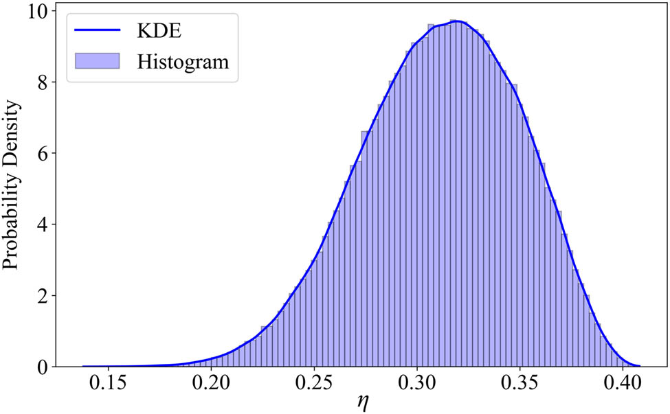
η distribution of κ ≥ 0.95.
3 Process of nonlinear comprehensive evaluation method based on information entropy and discrimination optimization
The proposed method is essentially an improvement of known evaluation methods given the evaluation dataset and indicator weights. By eliminating qualification and invalid indicators from the evaluation indicators and weighting only the weighted indicators, it ensures that the evaluation has good comprehensive evaluation discriminability.
In specific applications of comprehensive evaluation, if there are a large number of qualification and invalid indicators, it can affect the comprehensiveness of the evaluation. In such cases, the first step is to check the scientific nature of the quantification of the datasets corresponding to the qualification and invalid indicators. The second step is to introduce a parameter decrease rate coefficient λ (set λ = 0.8 to ensure the continuity and stability of the threshold variation.) for dynamic adjustment of the parameters α and β. Specifically, if the cumulative weight of invalid indicators exceeds 0.2, update the threshold α ← λα to increase the number of weighted indicators, and update the threshold β ← λβ to reduce the number of invalid indicators, thereby meeting the requirements for the comprehensiveness of the evaluation. The pseudocode of the proposed method is illustrated in Figure 3.
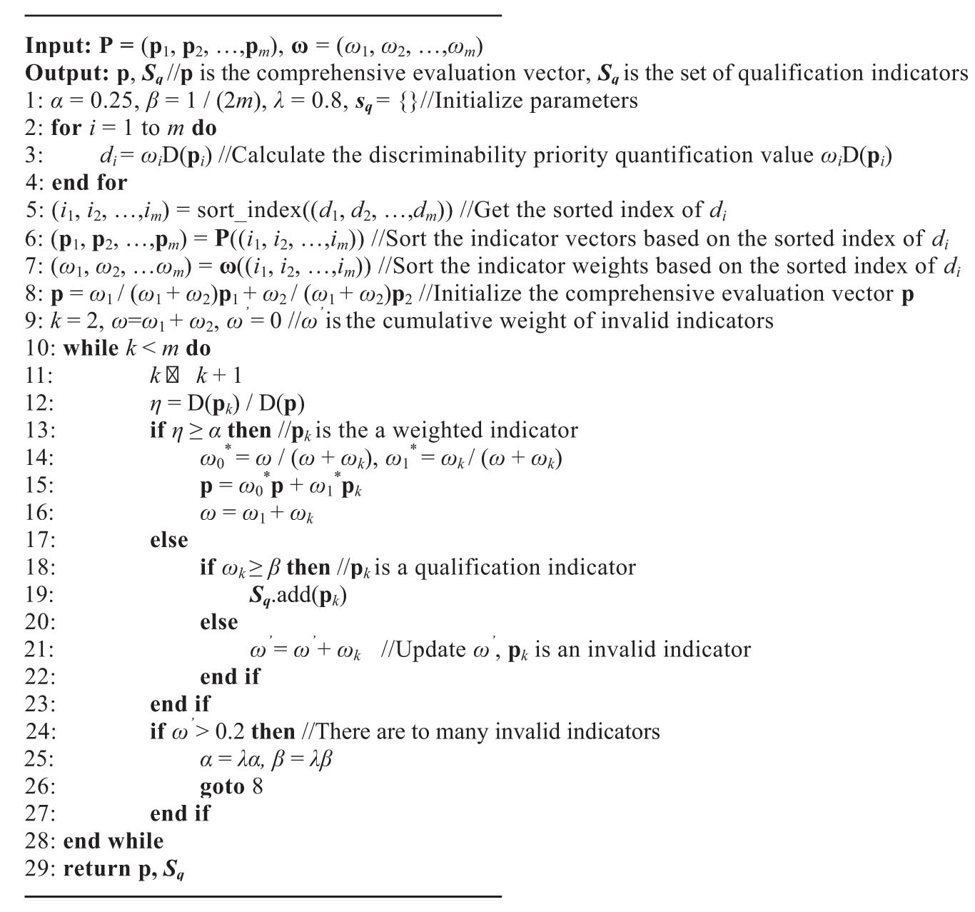
Pseudocode of the proposed method.
4 Case study
In this section, the proposed method is applied to comprehensive evaluations using both material selection evaluation data and synthetic evaluation data. The results are compared with those from conventional methods to verify whether the proposed method meets the expected standards in terms of discriminability and effectiveness of the evaluation.
4.1 Die-casting magnesium alloys selection evaluation
The material selection process involves numerous factors, necessitating a comprehensive evaluation of materials based on various performance aspects. Taking the selection of magnesium alloy materials as an example, this section evaluates five widely used magnesium alloys – AZ91, AM60, AM20, AE42, and AS41 – from the AZ (Mg–Al–Zn), AM (Mg–Al–Mn), AS (Mg–Al–Si), and AE (Mg–Al–Re) series, based on 21 indicators across three aspects: service performance, technological performance, and eco-economic performance. The weights of the indicators are shown in Table 1, and the specific indicator values can be found in ref. [4].
Evaluation indicators and weights for die-casting magnesium alloy selection
| No. | Primary indicator | Secondary indicator | Weight | No. | Primary indicator | Secondary indicator | Weight |
|---|---|---|---|---|---|---|---|
| 1 | Service performance | Oxidation activity | 0.1531 | 11 | Technological performance | Resistance to cold defects | 0.0401 |
| 2 | Corrosion resistance | 0.1435 | 12 | Air-tightness | 0.0453 | ||
| 3 | Impact toughness (J) | 0.0653 | 13 | Hot cracking sensitivity | 0.0212 | ||
| 4 | Strength (MPa) | 0.0799 | 14 | Flowability | 0.0119 | ||
| 5 | Stiffness (GPa) | 0.0480 | 15 | Non-Adhesion to molds | 0.0119 | ||
| 6 | Elongation | 0.0480 | 16 | Machinability | 0.0071 | ||
| 7 | Polishability | 0.0292 | 17 | Surface treatment capability | 0.0918 | ||
| 8 | Damping capability | 0.0118 | 18 | Plating performance | 0.0290 | ||
| 9 | Thermal conductivity | 0.0036 | 19 | Eco-economic performance | Environmental friendliness | 0.0327 | |
| 10 | Electrical conductivity | 0.0545 | 20 | Recyclability and reusability | 0.0394 | ||
| 21 | Economic viability | 0.0327 |
In the original evaluation, there were 21 secondary indicators. However, only 14 weighted indicators were actually involved in the evaluation. Among them, indicators 2, 12, 17, 19, and 20 are qualification indicators, while indicators 8 and 15 are invalid indicators. Table 2 presents the comparative results of the comprehensive evaluation of the five die-casting magnesium alloys. In addition to the discriminability defined by Eq. (3), the discriminability index defined by Eq. (1) (with a weight of 33%) and the discriminability function defined by Eq. (2) were introduced for comparative analysis. The improvement percentages of the three types of discriminability definitions are 210, 55, and 87%, respectively.
Comparative result of the comprehensive evaluation of die-casting magnesium alloys
| Magnesium alloy | AZ91 | AM60 | AM20 | AE42 | AS41 |
|---|---|---|---|---|---|
| Proposed method | 0.2527 | 0.2167 | 0.1642 | 0.2161 | 0.1503 |
| Original method | 0.2336 | 0.2165 | 0.1763 | 0.2102 | 0.1633 |
| Comprehensive ranking | 1 | 2 | 4 | 3 | 5 |
| Qualification indicators (Grade ≥ 4) | Meets | Meets | Meets | Meets | Meets |
As shown in Table 2 and Figure 4, the comprehensive evaluation ranking results obtained using the proposed method are consistent with those of the original evaluation. However, the discriminability of the evaluation results is significantly enhanced. Consequently, the proposed method can accurately identify invalid indicators in comprehensive evaluations. If no qualification or invalid indicators are identified during the evaluation process, the proposed method will not alter the evaluation results. This also indicates that the original method already possesses good comprehensive evaluation discriminability.
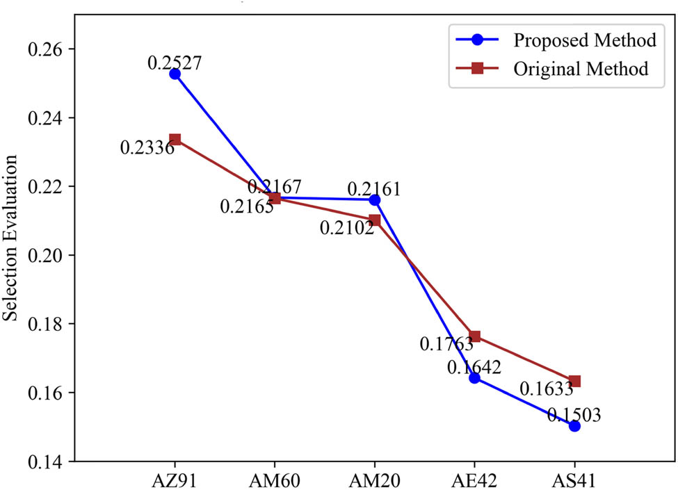
Comparison of the comprehensive evaluation of die-casting magnesium alloys.
4.2 Synthetic data comprehensive evaluation
In accordance with the experimental design for analyzing the rationality of the initial threshold value α = 0.25 presented in Section 2.3, 10,00,000 sets of randomly generated data are used as simulated evaluation data for further experiments on discriminability enhancement and evaluation validity.
The median values of discriminability enhancement for the proposed discriminability, the discriminability from Reference [8], the 27% discriminability index, and the 33% discriminability index are 26.2, 11.5, 9.6, and 9.6%, respectively. The results of the discriminability enhancement distributions are presented in Figure 5.
![Figure 5
Discriminability improvement of synthetic data evaluation. (a) Proposed discriminability improvement (%). (b) Ref. [8] discriminability improvement (%). (c) Discriminability index (27%) improvement. (d) Discriminability index (33%) improvement.](/document/doi/10.1515/nleng-2025-0154/asset/graphic/j_nleng-2025-0154_fig_005.jpg)
Discriminability improvement of synthetic data evaluation. (a) Proposed discriminability improvement (%). (b) Ref. [8] discriminability improvement (%). (c) Discriminability index (27%) improvement. (d) Discriminability index (33%) improvement.
The validity of the proposed method is demonstrated through a Cohen’s kappa consistency test comparing the evaluation results of the proposed method and the original method on synthetic data. Figure 6 shows that among all the test data, 60.8% have κ = 1, 94.48% have κ ≥ 0.95, and 99.9% have κ ≥ 0.8.
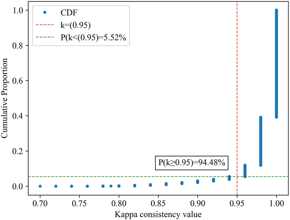
Cumulative distribution function of synthetic data Cohen’s kappa consistency test.
5 Conclusion
This article first defines a discriminability quantification method based on information entropy, which has a clear physical meaning and does not require sorting of evaluation results during the calculation process, making it easier to derive related conclusions theoretically. Moreover, the indicator discriminability can reflect the scientific nature of the evaluation indicator quantification to a certain extent. Subsequently, it is proven that the comprehensive evaluation discriminability decreases as low-discriminability evaluation indicators are added, and the lower bound estimation of the rate of decrease in comprehensive evaluation discriminability is provided, laying the theoretical foundation for the method presented in this article. Qualitative analysis and numerical experiments are conducted to establish the classification criteria for weighted indicators, qualification indicators, and invalid indicators. Based on this, a nonlinear comprehensive evaluation method based on information entropy and discrimination optimization is proposed, which involves weighting only the weighted indicators to calculate the evaluation results. Finally, this method is applied to case studies of comprehensive evaluation using die-casting magnesium alloys performance data and randomly generated data. Through qualitative analysis and practical application, it is evident that the proposed method has a definite comprehensive evaluation discriminability and reliable effectiveness. In numerical experiments, the deviation in the high-scoring partition significantly increases, effectively reducing the chances of repeated scores in comprehensive evaluations, making it particularly suitable for selective comprehensive evaluations. In future research, the indicator classification method and the selection of method parameters can be further optimized using machine learning algorithms [20].
Acknowledgments
The authors acknowledge the Ministry of Education Humanities and Social Sciences Project (Grant: 23YJA880061), the First Batch of Teaching Reform Projects in the 14th Five-Year Plan of Higher Vocational Education in Zhejiang Province (Grant: jg20230410), and the Second Batch of Teaching Reform Projects in the 14th Five-Year Plan of Higher Vocational Education in Zhejiang Province (Grant: jg20240410).
-
Funding information: The authors state no funding involved.
-
Author contributions: Guanjun Xu: funding acquisition, conceptualization, investigation, methodology, writing – original draft. Xijun Zeng: data curation, formal analysis, validation, writing – review and editing. All authors have accepted responsibility for the entire content of this manuscript and approved its submission.
-
Conflict of interest: The authors state no conflict of interest.
-
Data availability statement: The data sets used and/or analyzed during the current study are available from the corresponding author on reasonable request.
References
[1] Riedel SL, Pitz GF. Utilization-oriented evaluation of decision support systems. IEEE Trans Man Cybern. 1986;16(6):980–96.10.1109/TSMC.1986.4309016Search in Google Scholar
[2] Du D, Pang QH. Modern comprehensive evaluation method and case selection. Beijing: Tsinghua University Press; 2021.Search in Google Scholar
[3] Sun JS, Wang X, Zeng DZ, Yang J, Li ZL, Luo JC, et al. A method for evaluating the applicability of nickel-based alloy tubing/casing in high-temperature, high-pressure, and high-sulfur gas wells. Nat Gas Ind J. 2024;44(11):1–10.Search in Google Scholar
[4] Zhao JH, Duan YL, Chu WH. Improve analysis hierarchy process and fuzzy synthetic judgment on the selection of die casting magnesium alloys. Die Cast Res. 2008;29(6):735–8.Search in Google Scholar
[5] Kaliszewski I, Podkopaev D. Simple additive weighting - A metamodel for multiple criteria decision analysis methods. Expert Syst Appl. 2016;54:155–61.10.1016/j.eswa.2016.01.042Search in Google Scholar
[6] Butler JD, Morrice DJ, Mullarkey PW. A multiple attribute utility theory approach to ranking and selection. Manag Sci. 2001;47(6):800–16.10.1287/mnsc.47.6.800.9812Search in Google Scholar
[7] Peng ZL, Zhang Q, Yang SL. Overview of comprehensive evaluation theory and methodology. Chin J Manag Sci. 2015;23(SI):245–56.Search in Google Scholar
[8] Li XQ, Gao XH. Research on the optimal dimensionless model in comprehensive evaluation methods. Stat Decis. 2024;40(5):44–9.Search in Google Scholar
[9] Li H, Zhu JP. Research progress on comprehensive evaluation methods. Stat Decis. 2012;9:7–11.Search in Google Scholar
[10] Saaty TL. Axiomatic foundation of the analytic hierarchy process. Manag Sci. 1986;32(7):841–55.10.1287/mnsc.32.7.841Search in Google Scholar
[11] Zhang MF. Combination evaluation methods and applications. Beijing: Science Press; 2018.Search in Google Scholar
[12] Steiger NM, Wilson JR. An improved batch means procedure for simulation output analysis. Manag Sci. 2002;48(12):1569–86.10.1287/mnsc.48.12.1569.438Search in Google Scholar
[13] Weick KE. Theory construction as disciplined imagination. Acad Manag Rev. 1989;14(4):516–31.10.2307/258556Search in Google Scholar
[14] Cureton EE. The upper and lower twenty-seven percent rule. Psychometrika. 1957;22:293–6.10.1007/BF02289130Search in Google Scholar
[15] Guo YJ, Ma FM, Dong QX. Analysis of the influence of dimensionless methods on deviation maximization method. J Manag Sci China. 2011;14(5):19–28.Search in Google Scholar
[16] Zhang R, Liu SF, Liu B. A general algorithm for objective weighting based on deviation maximization. Stat Decis. 2007;24:29–31.Search in Google Scholar
[17] Li ZR, Ma XJ, Peng ZL. Research on combination evaluation methods based on deviation maximization. Chin J Manag Sci. 2013;21(1):174–9.Search in Google Scholar
[18] Li XQ, Gao XH. Research on discriminability and stability of comprehensive evaluation results. Stat Decis. 2022;38(16):16–21.Search in Google Scholar
[19] Li YN. Research on the distinguish degree and weight designing of evaluation system based on entropy theory [dissertation]. Nanjing: Nanjing University of Aeronautics and Astronautics; 2008.Search in Google Scholar
[20] Luo WY, Li M, Cai JJ. Research on multi-period development evaluation model for online learning based on XGBoost algorithm. Educ Inf Technol. 2024;24(6):49–54.Search in Google Scholar
© 2025 the author(s), published by De Gruyter
This work is licensed under the Creative Commons Attribution 4.0 International License.
Articles in the same Issue
- Research Articles
- Generalized (ψ,φ)-contraction to investigate Volterra integral inclusions and fractal fractional PDEs in super-metric space with numerical experiments
- Solitons in ultrasound imaging: Exploring applications and enhancements via the Westervelt equation
- Stochastic improved Simpson for solving nonlinear fractional-order systems using product integration rules
- Exploring dynamical features like bifurcation assessment, sensitivity visualization, and solitary wave solutions of the integrable Akbota equation
- Research on surface defect detection method and optimization of paper-plastic composite bag based on improved combined segmentation algorithm
- Impact the sulphur content in Iraqi crude oil on the mechanical properties and corrosion behaviour of carbon steel in various types of API 5L pipelines and ASTM 106 grade B
- Unravelling quiescent optical solitons: An exploration of the complex Ginzburg–Landau equation with nonlinear chromatic dispersion and self-phase modulation
- Perturbation-iteration approach for fractional-order logistic differential equations
- Variational formulations for the Euler and Navier–Stokes systems in fluid mechanics and related models
- Rotor response to unbalanced load and system performance considering variable bearing profile
- DeepFowl: Disease prediction from chicken excreta images using deep learning
- Channel flow of Ellis fluid due to cilia motion
- A case study of fractional-order varicella virus model to nonlinear dynamics strategy for control and prevalence
- Multi-point estimation weldment recognition and estimation of pose with data-driven robotics design
- Analysis of Hall current and nonuniform heating effects on magneto-convection between vertically aligned plates under the influence of electric and magnetic fields
- A comparative study on residual power series method and differential transform method through the time-fractional telegraph equation
- Insights from the nonlinear Schrödinger–Hirota equation with chromatic dispersion: Dynamics in fiber–optic communication
- Mathematical analysis of Jeffrey ferrofluid on stretching surface with the Darcy–Forchheimer model
- Exploring the interaction between lump, stripe and double-stripe, and periodic wave solutions of the Konopelchenko–Dubrovsky–Kaup–Kupershmidt system
- Computational investigation of tuberculosis and HIV/AIDS co-infection in fuzzy environment
- Signature verification by geometry and image processing
- Theoretical and numerical approach for quantifying sensitivity to system parameters of nonlinear systems
- Chaotic behaviors, stability, and solitary wave propagations of M-fractional LWE equation in magneto-electro-elastic circular rod
- Dynamic analysis and optimization of syphilis spread: Simulations, integrating treatment and public health interventions
- Visco-thermoelastic rectangular plate under uniform loading: A study of deflection
- Threshold dynamics and optimal control of an epidemiological smoking model
- Numerical computational model for an unsteady hybrid nanofluid flow in a porous medium past an MHD rotating sheet
- Regression prediction model of fabric brightness based on light and shadow reconstruction of layered images
- Dynamics and prevention of gemini virus infection in red chili crops studied with generalized fractional operator: Analysis and modeling
- Qualitative analysis on existence and stability of nonlinear fractional dynamic equations on time scales
- Fractional-order super-twisting sliding mode active disturbance rejection control for electro-hydraulic position servo systems
- Analytical exploration and parametric insights into optical solitons in magneto-optic waveguides: Advances in nonlinear dynamics for applied sciences
- Bifurcation dynamics and optical soliton structures in the nonlinear Schrödinger–Bopp–Podolsky system
- Review Article
- Haar wavelet collocation method for existence and numerical solutions of fourth-order integro-differential equations with bounded coefficients
- Special Issue: Nonlinear Analysis and Design of Communication Networks for IoT Applications - Part II
- Silicon-based all-optical wavelength converter for on-chip optical interconnection
- Research on a path-tracking control system of unmanned rollers based on an optimization algorithm and real-time feedback
- Analysis of the sports action recognition model based on the LSTM recurrent neural network
- Industrial robot trajectory error compensation based on enhanced transfer convolutional neural networks
- Research on IoT network performance prediction model of power grid warehouse based on nonlinear GA-BP neural network
- Interactive recommendation of social network communication between cities based on GNN and user preferences
- Application of improved P-BEM in time varying channel prediction in 5G high-speed mobile communication system
- Construction of a BIM smart building collaborative design model combining the Internet of Things
- Optimizing malicious website prediction: An advanced XGBoost-based machine learning model
- Economic operation analysis of the power grid combining communication network and distributed optimization algorithm
- Sports video temporal action detection technology based on an improved MSST algorithm
- Internet of things data security and privacy protection based on improved federated learning
- Enterprise power emission reduction technology based on the LSTM–SVM model
- Construction of multi-style face models based on artistic image generation algorithms
- Research and application of interactive digital twin monitoring system for photovoltaic power station based on global perception
- Special Issue: Decision and Control in Nonlinear Systems - Part II
- Animation video frame prediction based on ConvGRU fine-grained synthesis flow
- Application of GGNN inference propagation model for martial art intensity evaluation
- Benefit evaluation of building energy-saving renovation projects based on BWM weighting method
- Deep neural network application in real-time economic dispatch and frequency control of microgrids
- Real-time force/position control of soft growing robots: A data-driven model predictive approach
- Mechanical product design and manufacturing system based on CNN and server optimization algorithm
- Application of finite element analysis in the formal analysis of ancient architectural plaque section
- Research on territorial spatial planning based on data mining and geographic information visualization
- Fault diagnosis of agricultural sprinkler irrigation machinery equipment based on machine vision
- Closure technology of large span steel truss arch bridge with temporarily fixed edge supports
- Intelligent accounting question-answering robot based on a large language model and knowledge graph
- Analysis of manufacturing and retailer blockchain decision based on resource recyclability
- Flexible manufacturing workshop mechanical processing and product scheduling algorithm based on MES
- Exploration of indoor environment perception and design model based on virtual reality technology
- Tennis automatic ball-picking robot based on image object detection and positioning technology
- A new CNN deep learning model for computer-intelligent color matching
- Design of AR-based general computer technology experiment demonstration platform
- Indoor environment monitoring method based on the fusion of audio recognition and video patrol features
- Health condition prediction method of the computer numerical control machine tool parts by ensembling digital twins and improved LSTM networks
- Establishment of a green degree evaluation model for wall materials based on lifecycle
- Quantitative evaluation of college music teaching pronunciation based on nonlinear feature extraction
- Multi-index nonlinear robust virtual synchronous generator control method for microgrid inverters
- Manufacturing engineering production line scheduling management technology integrating availability constraints and heuristic rules
- Analysis of digital intelligent financial audit system based on improved BiLSTM neural network
- Attention community discovery model applied to complex network information analysis
- A neural collaborative filtering recommendation algorithm based on attention mechanism and contrastive learning
- Rehabilitation training method for motor dysfunction based on video stream matching
- Research on façade design for cold-region buildings based on artificial neural networks and parametric modeling techniques
- Intelligent implementation of muscle strain identification algorithm in Mi health exercise induced waist muscle strain
- Optimization design of urban rainwater and flood drainage system based on SWMM
- Improved GA for construction progress and cost management in construction projects
- Evaluation and prediction of SVM parameters in engineering cost based on random forest hybrid optimization
- Museum intelligent warning system based on wireless data module
- Optimization design and research of mechatronics based on torque motor control algorithm
- Special Issue: Nonlinear Engineering’s significance in Materials Science
- Experimental research on the degradation of chemical industrial wastewater by combined hydrodynamic cavitation based on nonlinear dynamic model
- Study on low-cycle fatigue life of nickel-based superalloy GH4586 at various temperatures
- Some results of solutions to neutral stochastic functional operator-differential equations
- Ultrasonic cavitation did not occur in high-pressure CO2 liquid
- Research on the performance of a novel type of cemented filler material for coal mine opening and filling
- Testing of recycled fine aggregate concrete’s mechanical properties using recycled fine aggregate concrete and research on technology for highway construction
- A modified fuzzy TOPSIS approach for the condition assessment of existing bridges
- Nonlinear structural and vibration analysis of straddle monorail pantograph under random excitations
- Achieving high efficiency and stability in blue OLEDs: Role of wide-gap hosts and emitter interactions
- Construction of teaching quality evaluation model of online dance teaching course based on improved PSO-BPNN
- Enhanced electrical conductivity and electromagnetic shielding properties of multi-component polymer/graphite nanocomposites prepared by solid-state shear milling
- Optimization of thermal characteristics of buried composite phase-change energy storage walls based on nonlinear engineering methods
- A higher-performance big data-based movie recommendation system
- Nonlinear impact of minimum wage on labor employment in China
- Nonlinear comprehensive evaluation method based on information entropy and discrimination optimization
- Application of numerical calculation methods in stability analysis of pile foundation under complex foundation conditions
- Research on the contribution of shale gas development and utilization in Sichuan Province to carbon peak based on the PSA process
- Characteristics of tight oil reservoirs and their impact on seepage flow from a nonlinear engineering perspective
- Nonlinear deformation decomposition and mode identification of plane structures via orthogonal theory
- Numerical simulation of damage mechanism in rock with cracks impacted by self-excited pulsed jet based on SPH-FEM coupling method: The perspective of nonlinear engineering and materials science
- Cross-scale modeling and collaborative optimization of ethanol-catalyzed coupling to produce C4 olefins: Nonlinear modeling and collaborative optimization strategies
- Unequal width T-node stress concentration factor analysis of stiffened rectangular steel pipe concrete
- Special Issue: Advances in Nonlinear Dynamics and Control
- Development of a cognitive blood glucose–insulin control strategy design for a nonlinear diabetic patient model
- Big data-based optimized model of building design in the context of rural revitalization
- Multi-UAV assisted air-to-ground data collection for ground sensors with unknown positions
- Design of urban and rural elderly care public areas integrating person-environment fit theory
- Application of lossless signal transmission technology in piano timbre recognition
- Application of improved GA in optimizing rural tourism routes
- Architectural animation generation system based on AL-GAN algorithm
- Advanced sentiment analysis in online shopping: Implementing LSTM models analyzing E-commerce user sentiments
- Intelligent recommendation algorithm for piano tracks based on the CNN model
- Visualization of large-scale user association feature data based on a nonlinear dimensionality reduction method
- Low-carbon economic optimization of microgrid clusters based on an energy interaction operation strategy
- Optimization effect of video data extraction and search based on Faster-RCNN hybrid model on intelligent information systems
- Construction of image segmentation system combining TC and swarm intelligence algorithm
- Particle swarm optimization and fuzzy C-means clustering algorithm for the adhesive layer defect detection
- Optimization of student learning status by instructional intervention decision-making techniques incorporating reinforcement learning
- Fuzzy model-based stabilization control and state estimation of nonlinear systems
- Optimization of distribution network scheduling based on BA and photovoltaic uncertainty
- Tai Chi movement segmentation and recognition on the grounds of multi-sensor data fusion and the DBSCAN algorithm
- Special Issue: Dynamic Engineering and Control Methods for the Nonlinear Systems - Part III
- Generalized numerical RKM method for solving sixth-order fractional partial differential equations