Qualitative analysis on existence and stability of nonlinear fractional dynamic equations on time scales
-
Kottakkaran Sooppy Nisar
 ,
Chandran Anusha
,
Chandran Anusha

Abstract
This study explores the qualitative analysis of
where
1 Introduction
A branch of mathematics that focuses on analyzing the integral and derivative operations for functions with fractional orders is known as fractional calculus, and it has gained momentum in recent years. It will be utilized in simulations and certain practical situations [1–8]. Indeed, it offers a multitude of valuable resources for resolving differential and integral equations, along with numerous other challenges related to specialized mathematical physics functions, including their expansions and advancements in both single and multiple variables [9–13]. In recent times, there has been an application of fractional differential equations (FDEs), for various practical issues, such as developing mathematical equations to describe the operation. In addition, FDEs along the integral boundary conditions are prevalent for various natural phenomena originating from diverse fields including fluid dynamics, chemical kinetics, electronics and bio models. Hence, numerous authors have investigated FDEs using various methodologies. The initial-boundary conditions are addressed using fixed point theorems and nonlinear functional analysis.
In 1990, Hilger proposed the introduction of time scales for combination and expansion upon existing differential equations (DEs), discrete equations, and other systems of DE defined upon a closed subset of real number line that is not empty [14–17]. The formulation of the initial value problem’s existence and uniqueness for DE on time scales is presented by Hilger along some practical uses. Combination of separate closed real intervals on time scales functions is a perfect structure to examine population dynamics. For past few years, there has been an increasing focus on time-dependent DEs (e.g., [18–21]). Time scales refer to a unified mathematical framework that integrates both discrete and continuous time, allowing for the examination of dynamic systems across varying types of intervals. This approach generalizes traditional DEs to include models that evolve in either continuous or discrete manners, thus broadening the scope of analysis in fractional dynamic systems. Similarly, integral boundary conditions require that solutions to DEs satisfy particular integral constraints rather than pointwise conditions at the boundaries. This is particularly relevant in real-world applications, where boundary conditions are often influenced by cumulative or averaged effects over time.
To decode both DEs and difference equations simultaneously, the dynamic equation is employed within a single domain known as time scale
Gogoi et al. [39], by application of the fixed point techniques, discussed the existence of solution of a nonlinear fractional dynamic equation with initial and boundary conditions on time scales. Motivated by the aforementioned work, using time scale we discuss the existence and stability results of a nonlinear fractional dynamic equation along the integral boundary condition,
where
2 Preliminaries
In the set of real numbers
for
A left dense-continuous function does not exist in
Definition 2.1
[40] If for every left dense point of
Space of ld-continuous function is set of every function from
Remark 2.2
Space function
for
Definition 2.3
[41] Consider
Definition 2.4
RL
Remark 2.5
From Definition 2.4, we also obtain
Definition 2.6
[43] Assume
Definition 2.7
[43] Assume a bounded set
Lemma 2.8
[44] Consider
Lemma 2.9
[45] Assume
Lemma 2.10
[46] (Krasnoselskii fixed point theorem) Assume a Banach space S. Consider
Lemma 2.11
[47] For
where
Definition 2.12
[47] Eq. (1.1) is known as Ulam–Hyer’s (UH) stable when there appears a constant
3 Main sequels
For the results of Eq. (1.1), we need some assumptions;
A function
There appears a constant
There appears a constant
A function
There appears a constant
There appears a constant
For
Assume a set
Theorem 3.1
Let ld-continuous function be
where
Proof
RL integral equation defines
which implies
Then, by Lemma 2.9, we have
Hence,
From integral boundary condition of Eq. (1.1) we have
Hence, we obtain
Subsequently, we obtain
Hence, the result follows.
Theorem 3.2
Assume (A1)–(A5) hold and
Eq. (1.1) contains unique solution.
Proof
For
Define
Here,
By using Lemma (2.8), we have
Hence,
Therefore,
Hence,
where
Therefore,
Theorem 3.3
Assume (A1) and (A2) hold, Eq. (1.1) contains atleast one solution, with assumptions is satisfied with
Proof
To prove the result, we take two maps
Here
Step 2: For each
Step 3: Define an operator
Here,
By using Lemma (2.8), we obtain
Hence,
Step 4: To prove the operator
Since functions
Therefore,
Step 5: Let
As
Theorem 3.4
Consider (A1)–(A5) and inequality (2.1) hold. Eq. (1.1) is UH stable.
Proof
Let
then by Theorem (1.1), we have
Then
Hence,
Thus,
where
Therefore, Eq. (1.1) is UH stable.
Setting
Therefore, Eq. (1.1) is generalized UH stable. Based on assumptions (A1)–(A5) and the validity of inequality (2.1), the unique solution
4 Nonlinear fractional dynamic equations (NFDE) with nonlocal condition
The research of nonlocal problems is driven by physical issues. As an illustration, it is employed to ascertain certain unidentified physical factors involved in inverse heat conduction problems. Byszewski first formulated and demonstrated the outcome regarding the presence and singularity of solutions to abstract Cauchy problems with nonlocal initial conditions. Many studies have discussed the subject of existence and uniqueness results in different kinds of nonlinear DEs. Initially, Byzewski formulated the nonlocal condition, where he mentioned [48], theorems about the existence and uniqueness of solutions of a semilinear evolution non-local Cauchy problem. Chang and Li [49] discussed the existence results for impulsive dynamic equations on time scales with nonlocal initial conditions. Subashini et al. [50] discussed the new results on nonlocal functional integro-DEs via Hilfer fractional derivative. Gogoi et al. [51] discussed the impulsive fractional dynamic equation with nonlocal initial condition on time scales. Inspired by the above work, we discuss the results for NFDE with nonlocal condition.
where
There appears a constant
There exists a constant
ensuring that the nonlocal term is bounded and does not introduce instability into the solution.
where
Theorem 4.1
Assume
Proof
Assume
By using the technique used in theorem 3.2, one can show that
5 Example
The following example serves as an illustration for our theoretical findings. To obtain the nonlinear problem (1.1) numerical solution, we will also provide the path of the proposed numerical scheme.
Example 5.1
Assume a fractional dynamic equation having the nonlinear integral boundary condition on time scale
where
satisfying the condition
Therefore, Eq. (5.1) has a solution at the interval
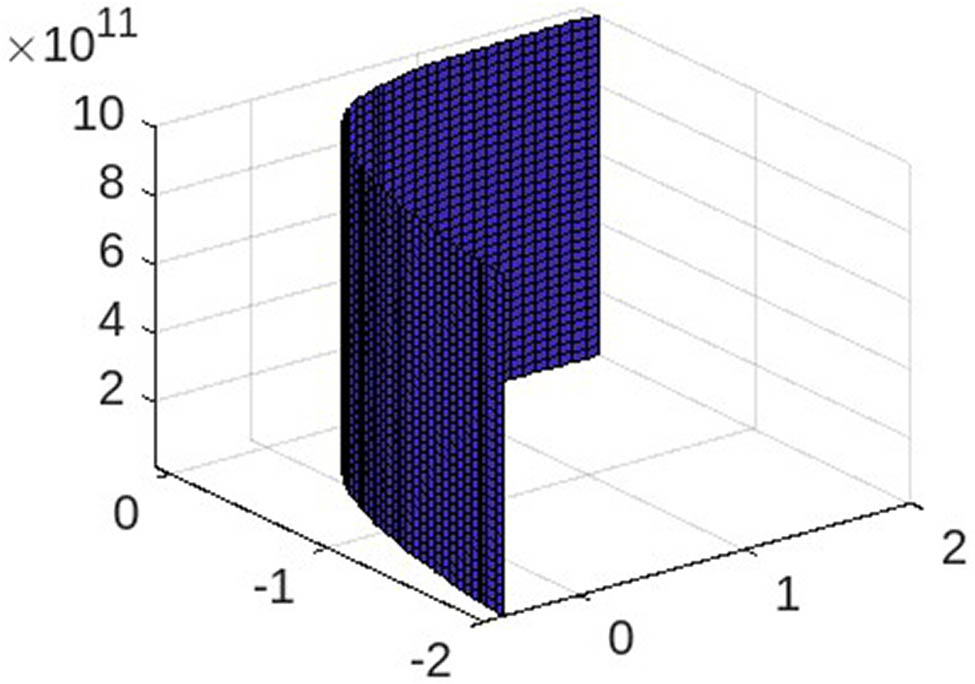
Graph of the approximate solution of
6 Conclusion
This study explores nonlinear fractional dynamic systems governed by RL nabla FDEs with integral boundary conditions. We established the existence, uniqueness, and stability of solutions using Krasnoselskii’s fixed point theorem and the Banach contraction principle, enhancing the applicability of our results to real-world systems. Our MATLAB-supported example highlights the practical implications of these findings.
These contributions deepen the understanding of fractional dynamic systems, offering insights for mathematicians and engineers in complex modeling. Future research will focus on advanced numerical methods, innovative control strategies, and applications in emerging technologies, laying a strong foundation for further advancements in fractional calculus.
Acknowledgments
The authors extend their appreciation to Prince Sattam bin Abdulaziz University, Saudi Arabia for funding this research work through the project number (PSAU/2025/R/1446).
-
Funding information: Authors state no funding involved.
-
Author contributions: All authors have accepted responsibility for the entire content of this manuscript and approved its submission.
-
Conflict of interest: Authors state no conflict of interest.
-
Data availability statement: All data generated or analysed during this study are included in this published article.
References
[1] Hioual A, Ouannas A, Grassi G, Oussaeif TE. Nonlinear nabla variable-order fractional discrete systems: Asymptotic stability and application to neural networks. J Comput Appl Math. 2023;423:114939. Suche in Google Scholar
[2] Jothimani K, Ravichandran C, Kumar V, Djemai M, Nisar KS. Interpretation of trajectory control and optimization for the nondense fractional system. Int J Appl Comput Math. 2022;8(6):273. Suche in Google Scholar
[3] Mohammed PO, Baleanu D, Abdeljawad T, Al-Sarairah E, Hamed YS. Monotonicity and extremality analysis of difference operators in Riemann–Liouville family. AIMS Math. 2023;8;5303–17. Suche in Google Scholar
[4] Ravichandran C, Sowbakiya V, Nisar KS. Study on existence and data dependence results for fractional order differential equations. Chaos Solitons Fractals. 2022;160:112232. Suche in Google Scholar
[5] Paul SK, Mishra LN, Mishra VN, Baleanu D. An effective method for solving nonlinear integral equations involving the Riemann–Liouville fractional operator. AIMS Math. 2023;8:17448–69. Suche in Google Scholar
[6] Nisar KS, Anusha C, Ravichandran C. A non-linear fractional neutral dynamic equations: existence and stability results on time scales. AIMS Math. 2024;9(1):1911–25. Suche in Google Scholar
[7] Kaliraj K. An investigation of fractional mixed functional integro-differential equations with impulsive conditions. Discontinuity Nonlinearity Complexity. 2024;13(01):189–202. Suche in Google Scholar
[8] Munusamy K, Ravichandran C, Nisar KS, Munjam SR. Investigation on continuous dependence and regularity solutions of functional integrodifferential equations. Results Control Optim. 2024;14:100376. Suche in Google Scholar
[9] Zhu J, Wu L. Fractional Cauchy problem with Caputo nabla derivative on time scales. In: Abstract and applied analysis. Vol. 2015. No. 1. Egypt: Hindawi Publishing Corporation; 2015. p. 486054. Suche in Google Scholar
[10] Benchohra M, Ouaar F. Existence results for nonlinear fractional differential equations with integral boundary conditions. Bull Math Anal Appl. 2010;2(4):7–15. Suche in Google Scholar
[11] Mohiuddine SA, Das A, Alotaibi A. Existence of solutions for nonlinear integral equations in tempered sequence spaces via generalized Darbo-type theorem. J Funct Spaces. 2022;2022(1):4527439. Suche in Google Scholar
[12] Veeresha P, Prakasha DG, Ravichandran C, Akinyemi L, Nisar KS. Numerical approach to generalized coupled fractional Ramani equations. Int J Modern Phys B. 2022;36(05):2250047. Suche in Google Scholar
[13] Wei Y, Zhao X, Wei Y, Chen Y. Lyapunov stability analysis for incommensurate nabla fractional order systems. J Syst Sci Complexity. 2023;36(2):555–76. Suche in Google Scholar
[14] Kumar V, Djemai M, Defoort M, Malik M. Total controllability results for a class of time-varying switched dynamical systems with impulses on time scales. Asian J Control. 2022;24(1):474–82. Suche in Google Scholar
[15] Kumar V, Malik M. Controllability results of fractional integro-differential equation with non-instantaneous impulses on time scales. IMA J Math Control Inform. 2021;38(1):211–31. Suche in Google Scholar
[16] Kumar V, Malik M. Existence and stability results of nonlinear fractional differential equations with nonlinear integral boundary condition on time scales. Appl Appl Math Int J (AAM). 2020;15(3):10. Suche in Google Scholar
[17] Kumar V, Malik M. Existence stability and controllability results of fractional dynamic system on time scales with application to population dynamics. Int J Nonl Sci Numer Simulat. 2021;22(6):741–66. Suche in Google Scholar
[18] Agarwal RP, O’Regan D. Nonlinear boundary value problems on time scales. Nonl Anal Theory Methods Appl. 2001;44(4):527–35. Suche in Google Scholar
[19] Bendouma B, Cherif AB, Hammoudi A. Existence of solutions for nonlocal nabla conformable fractional thermistor problem on time scales. Mem Differ Equ Math Phys. 2023;88:73–87. Suche in Google Scholar
[20] Benkhettou N, Hammoudi A, Torres DF. Existence and uniqueness of solution for a fractional Riemann–Liouville initial value problem on time scales. J King Saud Univ-Sci. 2016;28(1):87–92. Suche in Google Scholar
[21] Kaliraj K, Priya PL, Ravichandran C. An explication of finite-time stability for fractional delay model with neutral impulsive conditions. Qualitative Theory Dynam Syst. 2022;21(4):161. Suche in Google Scholar
[22] Agarwal R, Bohner M, O’Regan D, Peterson A. Dynamic equations on time scales: a survey. J Comput Appl Math. 2002;141(1–2):1–26. Suche in Google Scholar
[23] Mahdi NK, Khudair AR. Stability of nonlinear q-fractional dynamical systems on time scale. Partial Differ Equ Appl Math. 2023;7:100496. Suche in Google Scholar
[24] Bohner M, Peterson A. Dynamic equations on time scales: An introduction with applications. Boston: Springer Science & Business Media; 2001. Suche in Google Scholar
[25] Bohner M, Peterson AC. Advances in dynamic equations on time scales. Birkäuser Boston. Inc ., Boston, MA. 2003. Suche in Google Scholar
[26] Sarkar N, Sen M, Saha D, Hazarika B. A qualitative study on fractional logistic integro-differential equations in an arbitrary time scale. Kragujevac J Math. 2026;50(3):403–14. Suche in Google Scholar
[27] Tian Z. Analysis and research on chaotic dynamics behaviour of wind power time series at different time scales. J Ambient Intel Human Comput. 2023;14(2):897–921. Suche in Google Scholar
[28] Ilhan E, Veeresha P, Baskonus HM. Fractional approach for a mathematical model of atmospheric dynamics of CO2 gas with an efficient method. Chaos Solitons Fractals. 2021;152:111347. Suche in Google Scholar
[29] Veeresha P. The efficient fractional order based approach to analyze chemical reaction associated with pattern formation. Chaos Solitons Fractals. 2022;165:112862. Suche in Google Scholar
[30] Sherly K, Veeresha P. Mathematical model for effective CO2 emission control with forest biomass using fractional operator. Model Earth Syst Environ. 2024;10(4):5469–88. Suche in Google Scholar
[31] Baishya C, Achar SJ, Veeresha P, Kumar D. Dynamical analysis of fractional yellow fever virus model with efficient numerical approach. J Comput Anal Appl. 2023;31(1):140–57.Suche in Google Scholar
[32] Boutiara A, Abdo MS, Benbachir M. Existence results for ψ-Caputo fractional neutral functional integro-differential equations with finite delay. Turkish J Math. 2020;44(6):2380–401. Suche in Google Scholar
[33] Wahash HA, Abdo M, Panchal SK. Existence and stability of a nonlinear fractional differential equation involving a ψ-Caputo operator. Adv Theory Nonl Anal Appl. 2020;4(4):266–78. Suche in Google Scholar
[34] Derbazi C, Baitiche Z, Abdo MS, Abdeljawad T. Qualitative analysis of fractional relaxation equation and coupled system with ψ-Caputo fractional derivative in Banach spaces. AIMS Math. 2021;6(3):2486–509. Suche in Google Scholar
[35] Goufo EF, Ravichandran C, Birajdar GA. Self-similarity techniques for chaotic attractors with many scrolls using step series switching. Math Model Anal. 2021;26(4):591–611. Suche in Google Scholar
[36] Nisar KS, Jagatheeshwari R, Ravichandran C, Veeresha P. High performance computational method for fractional model of solid tumour invasion. Ain Shams Eng J. 2023;14(12):102226. Suche in Google Scholar
[37] Ma YK, Dineshkumar C, Vijayakumar V, Udhayakumar R, Shukla A, Nisar KS. Approximate controllability of Atangana-Baleanu fractional neutral delay integrodifferential stochastic systems with nonlocal conditions. Ain Shams Eng J. 2023;14(3):101882. Suche in Google Scholar
[38] Ma YK, Dineshkumar C, Vijayakumar V, Udhayakumar R, Shukla A, Nisar KS. Hilfer fractional neutral stochastic Sobolev-type evolution hemivariational inequality: Existence and controllability. Ain Shams Eng J. 2023;14(9):102126. Suche in Google Scholar
[39] Gogoi B, Saha UK, Hazarika B. Existence of solution of a nonlinear fractional dynamic equation with initial and boundary conditions on time scales. J Anal. 2024;32(1):85–102. Suche in Google Scholar
[40] Gogoi B, Saha UK, Hazarika B, Torres DF, Ahmad H. Nabla fractional derivative and fractional integral on time scales. Axioms. 2021;10(4):317. Suche in Google Scholar
[41] Guseinov GS. Integration on time scales. J Math Anal Appl. 2003;285(1):107–27. Suche in Google Scholar
[42] Anastassiou GA. Foundations of nabla fractional calculus on time scales and inequalities. Comput Math Appl. 2010;59(12):3750–62. Suche in Google Scholar
[43] Tikare S, Tisdell CC. Nonlinear dynamic equations on time scales with impulses and nonlocal conditions. J Class Anal. 2020;16(2):125–40. Suche in Google Scholar
[44] Feng M, Zhang X, Li X, Ge W. Necessary and sufficient conditions for the existence of positive solution for singular boundary value problems on time scales. Adv Differ Equ. 2009;2009:1–4. Suche in Google Scholar
[45] Sahir MJ. Coordination of classical and dynamic inequalities complying on time scales. Eur J Math Anal. 2023;3:12. Suche in Google Scholar
[46] Morsy A, Nisar KS, Ravichandran C, Anusha C. Sequential fractional order neutral functional Integro differential equations on time scales with Caputo fractional operator over Banach spaces. AIMS Math. 2023;8(3):5934–49. Suche in Google Scholar
[47] Wang J, Fec M, Zhou Y. Ulam’s type stability of impulsive ordinary differential equations. J Math Anal Appl. 2012;395(1):258–64. Suche in Google Scholar
[48] Byszewski L. Theorems about the existence and uniqueness of solutions of a semilinear evolution nonlocal Cauchy problem. J Math Anal Appl. 1991;162(2):494–505. Suche in Google Scholar
[49] Chang YK, Li WT. Existence results for impulsive dynamic equations on time scales with nonlocal initial conditions. Math Comput Model. 2006;43(3–4):377–84. Suche in Google Scholar
[50] Subashini R, Jothimani K, Nisar KS, Ravichandran C. New results on nonlocal functional integro-differential equations via Hilfer fractional derivative. Alexandr Eng J. 2020;59(5):2891–9. Suche in Google Scholar
[51] Gogoi B, Hazarika B, Saha UK. Impulsive fractional dynamic equation with non-local initial condition on time scales. 2022 Jun 29. arXiv: http://arXiv.org/abs/arXiv:2207.01517. Suche in Google Scholar
© 2025 the author(s), published by De Gruyter
This work is licensed under the Creative Commons Attribution 4.0 International License.
Artikel in diesem Heft
- Research Articles
- Generalized (ψ,φ)-contraction to investigate Volterra integral inclusions and fractal fractional PDEs in super-metric space with numerical experiments
- Solitons in ultrasound imaging: Exploring applications and enhancements via the Westervelt equation
- Stochastic improved Simpson for solving nonlinear fractional-order systems using product integration rules
- Exploring dynamical features like bifurcation assessment, sensitivity visualization, and solitary wave solutions of the integrable Akbota equation
- Research on surface defect detection method and optimization of paper-plastic composite bag based on improved combined segmentation algorithm
- Impact the sulphur content in Iraqi crude oil on the mechanical properties and corrosion behaviour of carbon steel in various types of API 5L pipelines and ASTM 106 grade B
- Unravelling quiescent optical solitons: An exploration of the complex Ginzburg–Landau equation with nonlinear chromatic dispersion and self-phase modulation
- Perturbation-iteration approach for fractional-order logistic differential equations
- Variational formulations for the Euler and Navier–Stokes systems in fluid mechanics and related models
- Rotor response to unbalanced load and system performance considering variable bearing profile
- DeepFowl: Disease prediction from chicken excreta images using deep learning
- Channel flow of Ellis fluid due to cilia motion
- A case study of fractional-order varicella virus model to nonlinear dynamics strategy for control and prevalence
- Multi-point estimation weldment recognition and estimation of pose with data-driven robotics design
- Analysis of Hall current and nonuniform heating effects on magneto-convection between vertically aligned plates under the influence of electric and magnetic fields
- A comparative study on residual power series method and differential transform method through the time-fractional telegraph equation
- Insights from the nonlinear Schrödinger–Hirota equation with chromatic dispersion: Dynamics in fiber–optic communication
- Mathematical analysis of Jeffrey ferrofluid on stretching surface with the Darcy–Forchheimer model
- Exploring the interaction between lump, stripe and double-stripe, and periodic wave solutions of the Konopelchenko–Dubrovsky–Kaup–Kupershmidt system
- Computational investigation of tuberculosis and HIV/AIDS co-infection in fuzzy environment
- Signature verification by geometry and image processing
- Theoretical and numerical approach for quantifying sensitivity to system parameters of nonlinear systems
- Chaotic behaviors, stability, and solitary wave propagations of M-fractional LWE equation in magneto-electro-elastic circular rod
- Dynamic analysis and optimization of syphilis spread: Simulations, integrating treatment and public health interventions
- Visco-thermoelastic rectangular plate under uniform loading: A study of deflection
- Threshold dynamics and optimal control of an epidemiological smoking model
- Numerical computational model for an unsteady hybrid nanofluid flow in a porous medium past an MHD rotating sheet
- Regression prediction model of fabric brightness based on light and shadow reconstruction of layered images
- Dynamics and prevention of gemini virus infection in red chili crops studied with generalized fractional operator: Analysis and modeling
- Qualitative analysis on existence and stability of nonlinear fractional dynamic equations on time scales
- Fractional-order super-twisting sliding mode active disturbance rejection control for electro-hydraulic position servo systems
- Analytical exploration and parametric insights into optical solitons in magneto-optic waveguides: Advances in nonlinear dynamics for applied sciences
- Bifurcation dynamics and optical soliton structures in the nonlinear Schrödinger–Bopp–Podolsky system
- User profiling in university libraries by combining multi-perspective clustering algorithm and reader behavior analysis
- Review Article
- Haar wavelet collocation method for existence and numerical solutions of fourth-order integro-differential equations with bounded coefficients
- Special Issue: Nonlinear Analysis and Design of Communication Networks for IoT Applications - Part II
- Silicon-based all-optical wavelength converter for on-chip optical interconnection
- Research on a path-tracking control system of unmanned rollers based on an optimization algorithm and real-time feedback
- Analysis of the sports action recognition model based on the LSTM recurrent neural network
- Industrial robot trajectory error compensation based on enhanced transfer convolutional neural networks
- Research on IoT network performance prediction model of power grid warehouse based on nonlinear GA-BP neural network
- Interactive recommendation of social network communication between cities based on GNN and user preferences
- Application of improved P-BEM in time varying channel prediction in 5G high-speed mobile communication system
- Construction of a BIM smart building collaborative design model combining the Internet of Things
- Optimizing malicious website prediction: An advanced XGBoost-based machine learning model
- Economic operation analysis of the power grid combining communication network and distributed optimization algorithm
- Sports video temporal action detection technology based on an improved MSST algorithm
- Internet of things data security and privacy protection based on improved federated learning
- Enterprise power emission reduction technology based on the LSTM–SVM model
- Construction of multi-style face models based on artistic image generation algorithms
- Research and application of interactive digital twin monitoring system for photovoltaic power station based on global perception
- Special Issue: Decision and Control in Nonlinear Systems - Part II
- Animation video frame prediction based on ConvGRU fine-grained synthesis flow
- Application of GGNN inference propagation model for martial art intensity evaluation
- Benefit evaluation of building energy-saving renovation projects based on BWM weighting method
- Deep neural network application in real-time economic dispatch and frequency control of microgrids
- Real-time force/position control of soft growing robots: A data-driven model predictive approach
- Mechanical product design and manufacturing system based on CNN and server optimization algorithm
- Application of finite element analysis in the formal analysis of ancient architectural plaque section
- Research on territorial spatial planning based on data mining and geographic information visualization
- Fault diagnosis of agricultural sprinkler irrigation machinery equipment based on machine vision
- Closure technology of large span steel truss arch bridge with temporarily fixed edge supports
- Intelligent accounting question-answering robot based on a large language model and knowledge graph
- Analysis of manufacturing and retailer blockchain decision based on resource recyclability
- Flexible manufacturing workshop mechanical processing and product scheduling algorithm based on MES
- Exploration of indoor environment perception and design model based on virtual reality technology
- Tennis automatic ball-picking robot based on image object detection and positioning technology
- A new CNN deep learning model for computer-intelligent color matching
- Design of AR-based general computer technology experiment demonstration platform
- Indoor environment monitoring method based on the fusion of audio recognition and video patrol features
- Health condition prediction method of the computer numerical control machine tool parts by ensembling digital twins and improved LSTM networks
- Establishment of a green degree evaluation model for wall materials based on lifecycle
- Quantitative evaluation of college music teaching pronunciation based on nonlinear feature extraction
- Multi-index nonlinear robust virtual synchronous generator control method for microgrid inverters
- Manufacturing engineering production line scheduling management technology integrating availability constraints and heuristic rules
- Analysis of digital intelligent financial audit system based on improved BiLSTM neural network
- Attention community discovery model applied to complex network information analysis
- A neural collaborative filtering recommendation algorithm based on attention mechanism and contrastive learning
- Rehabilitation training method for motor dysfunction based on video stream matching
- Research on façade design for cold-region buildings based on artificial neural networks and parametric modeling techniques
- Intelligent implementation of muscle strain identification algorithm in Mi health exercise induced waist muscle strain
- Optimization design of urban rainwater and flood drainage system based on SWMM
- Improved GA for construction progress and cost management in construction projects
- Evaluation and prediction of SVM parameters in engineering cost based on random forest hybrid optimization
- Museum intelligent warning system based on wireless data module
- Optimization design and research of mechatronics based on torque motor control algorithm
- Special Issue: Nonlinear Engineering’s significance in Materials Science
- Experimental research on the degradation of chemical industrial wastewater by combined hydrodynamic cavitation based on nonlinear dynamic model
- Study on low-cycle fatigue life of nickel-based superalloy GH4586 at various temperatures
- Some results of solutions to neutral stochastic functional operator-differential equations
- Ultrasonic cavitation did not occur in high-pressure CO2 liquid
- Research on the performance of a novel type of cemented filler material for coal mine opening and filling
- Testing of recycled fine aggregate concrete’s mechanical properties using recycled fine aggregate concrete and research on technology for highway construction
- A modified fuzzy TOPSIS approach for the condition assessment of existing bridges
- Nonlinear structural and vibration analysis of straddle monorail pantograph under random excitations
- Achieving high efficiency and stability in blue OLEDs: Role of wide-gap hosts and emitter interactions
- Construction of teaching quality evaluation model of online dance teaching course based on improved PSO-BPNN
- Enhanced electrical conductivity and electromagnetic shielding properties of multi-component polymer/graphite nanocomposites prepared by solid-state shear milling
- Optimization of thermal characteristics of buried composite phase-change energy storage walls based on nonlinear engineering methods
- A higher-performance big data-based movie recommendation system
- Nonlinear impact of minimum wage on labor employment in China
- Nonlinear comprehensive evaluation method based on information entropy and discrimination optimization
- Application of numerical calculation methods in stability analysis of pile foundation under complex foundation conditions
- Research on the contribution of shale gas development and utilization in Sichuan Province to carbon peak based on the PSA process
- Characteristics of tight oil reservoirs and their impact on seepage flow from a nonlinear engineering perspective
- Nonlinear deformation decomposition and mode identification of plane structures via orthogonal theory
- Numerical simulation of damage mechanism in rock with cracks impacted by self-excited pulsed jet based on SPH-FEM coupling method: The perspective of nonlinear engineering and materials science
- Cross-scale modeling and collaborative optimization of ethanol-catalyzed coupling to produce C4 olefins: Nonlinear modeling and collaborative optimization strategies
- Unequal width T-node stress concentration factor analysis of stiffened rectangular steel pipe concrete
- Special Issue: Advances in Nonlinear Dynamics and Control
- Development of a cognitive blood glucose–insulin control strategy design for a nonlinear diabetic patient model
- Big data-based optimized model of building design in the context of rural revitalization
- Multi-UAV assisted air-to-ground data collection for ground sensors with unknown positions
- Design of urban and rural elderly care public areas integrating person-environment fit theory
- Application of lossless signal transmission technology in piano timbre recognition
- Application of improved GA in optimizing rural tourism routes
- Architectural animation generation system based on AL-GAN algorithm
- Advanced sentiment analysis in online shopping: Implementing LSTM models analyzing E-commerce user sentiments
- Intelligent recommendation algorithm for piano tracks based on the CNN model
- Visualization of large-scale user association feature data based on a nonlinear dimensionality reduction method
- Low-carbon economic optimization of microgrid clusters based on an energy interaction operation strategy
- Optimization effect of video data extraction and search based on Faster-RCNN hybrid model on intelligent information systems
- Construction of image segmentation system combining TC and swarm intelligence algorithm
- Particle swarm optimization and fuzzy C-means clustering algorithm for the adhesive layer defect detection
- Optimization of student learning status by instructional intervention decision-making techniques incorporating reinforcement learning
- Fuzzy model-based stabilization control and state estimation of nonlinear systems
- Optimization of distribution network scheduling based on BA and photovoltaic uncertainty
- Tai Chi movement segmentation and recognition on the grounds of multi-sensor data fusion and the DBSCAN algorithm
- Special Issue: Dynamic Engineering and Control Methods for the Nonlinear Systems - Part III
- Generalized numerical RKM method for solving sixth-order fractional partial differential equations