
Hydrodynamic and sensitivity analysis of a polymeric calendering process for non-Newtonian fluids with temperature-dependent viscosity
-
Fateh Ali
 ,
Muhammad Zahid
,
Muhammad Zahid

Abstract
Non-Newtonian fluids, particularly those with high viscosity and complex flow behavior, present unique challenges in manufacturing processes. The modeling of their flow dynamics is crucial to achieve the desired outcomes in industrial applications. This study aims to theoretically model and analyze the flow dynamics of the Eyring–Powell fluid under varying temperature conditions using lubrication approximation theory and perturbation method. To simplify the mathematical formulation of fluid flow motion, lubrication approximation theory is applied. Using a perturbation method, the dimensionless governing equations are solved to derive expressions for velocity, pressure gradient, and pressure distributions. Numerical integration is then used to calculate critical engineering parameters, such as power input and roll-separating force, offering practical insights for optimizing the manufacturing process. Additionally, using the response surface method, Nusselt number
Nomenclature
- U
-
velocity of the rollers
-
-
half of the nip region
-
-
viscosity parameter
-
-
radii of the roll
- ρ
-
fluid density
-
-
dimensionless leave off distance
-
-
perturb (small) parameter
- Br
-
Brinckmann number
-
-
roll separation force
-
-
power input
-
-
final sheet thickness
-
-
pressure gradient
-
-
pressure profile
-
-
temperature profile
1 Introduction
A fluid’s resistance to flow is highly influenced by temperature, pressure, and shear rate, all of which play crucial roles in determining the fluid’s behavior. The kinetic energy of fluid particles generates temperature within the fluid, and higher temperatures can significantly alter fluid properties, with viscosity being particularly sensitive to temperature increases. In fluids with variable viscosity, viscosity responds rapidly to changes in temperature, resulting in alterations to the fluid’s flow structure. Research on non-Newtonian fluids with temperature-dependent viscosity has been of significant interest for many years due to its importance in diverse industrial applications. This area encompasses a broad spectrum of phenomena relevant to processes such as oil drilling, food processing, and polymer manufacturing, where effective heat transfer is critical to operational efficiency and product quality. In these industrial settings, variations in viscosity can profoundly impact process efficiency and effectiveness. For example, understanding how viscosity varies with temperature can improve control over mixing uniformity and product consistency in fluid mixing applications. Thus, precise modeling and simulation of viscosity variations are essential for theoretical insights and for improving the design and efficiency of commercial operations, such as calendering [1].
The process of pulling molten polymer through the nip area in the middle of two sets of rotating rollers to create a sheet with a specific thickness is known as calendering. This process is integral to various industries, including textile, metal, paper, plastic, and tire manufacturing, where consistent material properties and controlled thickness are essential. Originating in the mid-nineteenth century, calendering technology was publicly demonstrated by inventors Edwin Chaffee and Charles Goodyear, marking a pivotal advancement in material processing. The first quantitative analysis of calendering, undertaken by [2] in 1938, introduced the application of lubrication approximation theory (LAT) within Newtonian hydrodynamics to address flow behavior at low Reynolds numbers, a regime typically encountered in calendering due to slow flow rates and narrow gaps. This analysis paved the way for more complex modeling approaches. Paslay’s [3] work on the Maxwell model in calendering further advanced the theoretical framework, assuming Weissenberg numbers less than one to account for the viscoelastic response of polymeric fluids under flow. Experimental insights also contributed significantly to calendering science. In 1951, Bergen and Scott [4] conducted pioneering measurements of internal pressure distribution within the calendering system, providing critical empirical data for model validation. Gaskell’s [5] study expanded upon this by offering the first theoretical analysis involving Bingham plastic and Newtonian fluids, noting that the interval width between rolls is negligible compared to the roll radii factor, which has considerable implications for flow stability and film uniformity. Thermal effects in calendering were subsequently addressed by Kiparissides and Vlachopoulos [6], who used a power-law fluid model to explore heat transfer dynamics. Their work involved solving the flow equations via the finite element method (FEM), showing strong agreement with experimental observations by Bergen and Scott, and highlighting the importance of temperature control in calendering applications. Tadmor and Gogos [7] and Brazinsky et al. [8] extended these analyses specifically for viscous power-law fluids commonly encountered in polymer processing, thus providing a comprehensive view of calendering flow behavior. Alston and Astill’s [9] study advanced the computational methods used in calendering analysis by employing a hyperbolic tangent model, combined in the company of Gauss–Legendre cartesian and cascade repetition, to quantify spread height and peak roller pressure, as well as their interdependencies. Theoretical advancements in the coating process have been extensively discussed in textbooks; interested readers may refer to these sources for further details [7,10,11]. Later, in 1988, Zheng and Tanner [12] applied the Phan–Thien–Tanner model to further elucidate the viscoelastic flow characteristics within the calendering mechanism, underscoring the impact of non-Newtonian behavior on the procedure.
Newtonian and power-law fluids in calendering were thoroughly examined by Mitsoulis et al. in a two-dimensional, non-isothermal framework. Mitsoulis et al. [13] using the FEM without employing the LAT. Later, Arcos et al. [14] explored the supremacy of various constants on sheet broadness in calendering using a temperature-dependent power-law fluid model, observing a 6.11% reduction in thickness compared to isothermal conditions. Sofou and Mitsoulis [15] extended this inquiry by simulating the finite sheet thickness calendering process for viscoplastic fluids modeled with the Herschel–Bulkley framework. A notable contribution by Hatzikiriakos [16] presented a numerical simulation focusing on the calendering of viscoplastic fluids, providing insights into material behavior under different calendering conditions. Arcos et al. [17] further advanced the understanding of calendering by employing a Newtonian fluid model that incorporated thermosensitive viscosity effects on sheet broadness. Within a separate investigation of non-isothermal flows in Casson fluids, Zahid et al. [18] addressed the complex thermal dynamics present in the calendering process. The work by Hernández et al. [19] examined a particular impact of pressure-dependent viscosity on sheet broadness at the exit of the calendering procedure, highlighting how pressure variations influence final product dimensions. Additionally, Arcos et al. [20] developed a theoretical model for calendering utilizing a more comprehensible Phan–Thien–Tanner essential equation beneath the lubrication approximation theory estimation. In investigating viscoelastic fluid dynamics, Ali et al. [21] scrutinize the effects of finitely extensible nonlinear elastic peterlin fluid (FENE-P) moisture in calendering, demonstrating significant viscoelastic influences on the process. Calcagno et al. [22] developed an analytical model for predicting pressure and tension profiles during calendering using Newtonian and power-law fluid assumptions. Their results aligned most closely with experimental findings when employing the Newtonian model. Most recently, Zahid et al. [23] presented a theoretical investigation on calendering with variable viscosity for third-grade model, analyzing how specific material properties influence the thickness of calendered sheets.
Most theoretical works in this dynamic research field concentrate on adhesive moisture; others are usually Newtonian. Numerous academics have included non-Newtonian vapors in their physically modeled issues, indicative of their widespread application in commercial settings. Here, theoretical investigation of non-Newtonian fluid dynamics is of primary interest [24]. A specific innumerable implementation of non-Newtonian in the technical, industrial, and commercial production sectors has increased interest in their study. Several authors have shown that non-Newtonian fluids apply to research [25]. Several studies have illustrated the various uses of non-Newtonian vapors. Several fluids collapse under this section, encompassing paper pulp, mayonnaise, cleaning agent, seashore, plastic melts, milk, and slurries. The Navier–Stokes identification can narrate the drizzle deportment of Newtonian fluids. Despite that, viscoelastic fluids’ flow behavior with all of its essential qualities is not in a position to be sufficiently narrated by a unique equation. Consequently, scientists and academics have proposed several non-Newtonian constitutive models. The viscoelastic fluid, power-law fluid, Cassion fluid, distinctive class fluid imitation, Sisko fluid, FENE-P fluid, Oldroyd family’s fluid, micropolar fluid, along with Eyring–Powell fluid, are a few examples of these patterns. We selected a specific Eyring–Powell fluid version, a non-Newtonian fluid imitation first presented among several fluid models [26,27]. This model performs better than previous viscoelastic fluid models in assorted areas. There are two main reasons why it offers many benefits. First, it uses the kinetic theory of object interactions instead of depending on the experimental formulas. Second, as is typical of Newtonian fluids, Eyring–Powell modeling responds to high and low shear rates. Researchers have talked a lot about the critical components of the Eyring–Powell fluid.
In the immediate years, there has been an extended use of experimental techniques to investigate the connections in the middle of free and response variables in complex systems. The hybrid statistical–mathematical approach known as response surface methodology (RSM) has gained significant traction among these methods. The primary objective of RSM is response optimization, which is particularly valuable for solving problems in heat transfer and fluid dynamics, as it aids in optimizing desired flow patterns. For instance, Darbari et al. [28] wore RSM to scrutinize a certain consequence of temperature and velocity on the standard Nusselt together with Reynolds numbers of nanofluids. Their study focused on nanofluids flowing through a straight, circular conduit under a steady thermal flux in the laminar regime. The RSM analysis revealed that temperature and velocity substantially impacted the dependent variables, with a notable interaction effect between these factors. As a result, RSM has become a widely adopted tool across various research domains for analyzing and optimizing complex interactions between multiple variables.
As far as we know and the scientific literature review, no attempt has yet been undertaken to analyze the calendering process using the Eyring–Powell model with viscosity temperature-dependent. Thus, the current work’s goal is to ascertain how, throughout the calendering process, the fluid parameter influences the leave distance, power input, velocity, final sheet thickness, and other quantities of engineering interest.
An examination of the structure and content of the literature mentioned earlier reveals several critical observations:
Numerous studies have explored the calendering process involving various non-Newtonian fluids, often assuming constant thermophysical properties. However, there remains a notable gap in research that explicitly addresses the impact of temperature-dependent viscosity, particularly in the context of Eyring–Powell fluids.
A significant number of studies fail to comprehensively analyze key engineering characteristics, such as sheet thickness, Nusselt number, shear stress, roll/sheet separating force, and power transmitted from the roll to the fluid. These parameters are crucial for optimizing industrial processes and ensuring high-quality outcomes.
Additionally, there is limited focus on the concurrent optimization of critical performance parameters, such as heat transfer rate, sheet thickness, and shear stress rate, which play a pivotal role in achieving efficient and effective manufacturing processes.
In light of these gaps identified through the literature review, the primary objectives of the present study are as follows:
To construct a robust mathematical model for the calendering process using an Eyring–Powell fluid with temperature-dependent viscosity, incorporating Reynold’s viscosity model to account for variable viscosity effects.
To investigate the influence of temperature-dependent viscosity on the dynamics of the calendering process, emphasizing its implications for real-world applications.
To examine the effects of pertinent parameters on critical engineering factors, including coating thickness, shear stress rate, heat transfer coefficient, roll/sheet separating force, and power transmitted from the roll to the fluid.
To identify and address the limitations associated with achieving dual optimization goals of the maximizing the heat transfer rate while minimizing the shear stress rate through the application of advanced optimization techniques.
Comparison of existing studies on the calendering process was made using different non-Newtonian fluid models and contributions of the present study.
| Author(s) | Fluid model | Process type | Limitations | Findings |
|---|---|---|---|---|
| Javed et al. [29] | Ellis fluid | Calendering | Did not consider temperature effects | Investigated coating performance at constant viscosity |
| Javed et al. [30] | Johnson–Segalman fluid | Calendering | Neglected magnetic field interactions | Did not consider variable viscosity |
| Abbas and Khaliq [31] | Cu–water nanofluid | Calendering | Did not consider RSM | Explored effects of different parameters on velocity and temperature, etc. |
| This study | Eyring–Powell fluid | Calendering | Ignore MHD and slip effects | Novelty: incorporates temperature-dependent viscosity with hybrid perturbation + RSM analysis for calendering process |
2 Problem description and governing equations
The following presumptions are expressed:
Figure 1 shows the calendering process sketch in which a non-Newtonian model’s thin film separates two rolls.
Since many materials used in calendering are frequently non-Newtonian, the Eyring–Powell model is considered to have temperature-dependent viscosity.
The radius of each calendar is
Figure 1 shows a small separation region between calendars known as the nip area, with a gap length of
Certain roll surfaces occur concerning a sustained temperature
Due to the symmetry of the physical model, we consider the upper side of this configuration only for convenience.

Illustrative depiction of the calendering procedure.
Without body forces, the momentum, mass, and energy equations are as follows [1,32]:
where
The following is the material derivative:
Scientists and engineers frequently reduce mathematical models to produce helpful approximations when working with complex physical systems. This procedure aims to improve comprehension of the physical system by emphasizing essential elements such as velocities, forces, fluxes, and other pertinent elements. We employ lubrication approximation theory in light of the aforementioned presumptions. The lubrication approximation theory indicates that the most significant dynamic events occur in the nip region, providing a basis for a thorough investigation.
The velocity profile of a balanced, incompressible, two-dimensional flow with laminar features can be noted as follows:
where a specific velocity component within the
2.1 Rheological model
The viscoelastic Eyring–Powell model’s description of the rheological characteristics is examined in this work. The following equations provide the Eyring–Powell model [33,34,35] in mathematical representation:
where
where
With the use of Eqs. (5) and (6), the constituent appearance of the governing equations is written as follows:
By applying the Taylor augmentation to the inverse hyperbolic expression in Eq. (6), we obtain the non-zero shear stress component in the simplified version as follows:
The following are the boundary conditions (BCs) in the proportion configuration linked to Eqs. (10)–(12):
For the
The pressure, velocity, and fluid temperature profiles are represented by the letters
We do an order of magnitude study to quickly determine the typical temperature, pressure, and velocity scales. The following scales for
Considering a particular mass conservation identity, Eq. (1), as well as a certain connection outlined over Eq. (15), we conclude that
According to a specific connection exceeding the longitudinal predictable length, represented by
2.2 Non-dimensionalities, together with the lubrication approximation theory
Non-dimensional restriction can simplify complicated fluid flow problems and provide insightful information; they are highly significant in various scientific and engineering domains. Physical occurrences. This segment offers the dimensionless identities required to work through the non-isothermal calendering process. We identify the following non-dimensional variables based on the order of magnitude analysis from earlier [10]:
Eqs. (9)–(13) are modified to provide the two-dimensional equations in dimensionless form by applying Eq. (17):
Because of Eq. (22), Eqs. (19) and (21) yield
The following are the relationships for the non-dimensional variables over Eq. (23) as well as (24):
where
3 Viscosity model
Unique patterns are selected to depict a specific fluid according to its viscosity. In particular, the viscosity is a function of the fluid’s temperature, and the imitation, as mentioned earlier, is known as a specific Reynolds model.
3.1 Reynolds model
To describe a given Reynolds dummy, a dummy with fluctuating viscosity, we shall ascertain a particular viscosity worth in terms of temperature as follows:
where (
Based on the previously described presumptions, the equation relating to motion and heat is defined as
BCs are [10]
The expression for flow rate in dimensionless form, which will help to find the value of pressure gradient, can be corresponded in the formation as [10]:
The approach of Eq. (28) along with (29) represents the prominent lubrication estimation [17] for Eyring–Powell fluid accompanied by thermosensitive viscosity. It must be esteemed that these identities are coupled and nonlinear. So, in the following section, we prevail the proportionate velocity, pressure gradient, pressure, and temperature profiles by solving Eqs. (28) and (29) with the help of BCs given in Eq. (30) using the perturbation method.
4 Asymptotic solution for
We
≪
1
To find the sheet thickness, pressure, detachment point, temperature distribution, and dimensionless velocity profile, Eqs. (28) and (29) have no exact solution; we try to determine an asymptotic solution, using
where the leading-order solutions
4.1 Zero-order problem and its solution
The first-order partition value dilemma
BCs are
The solution of Eq. (37) with help of BCs given in Eq. (38) is as follows:
The zeroth-order pressure gradient is as follows:
From the aforementioned equation, the zero-order pressure is
The exceeding mathematical form is uncoordinated in
For this value of
4.2 First-order complication and its emulsion
The first-order boundary value obstacle
BCs [10] are
The solution of Eq. (43) with aforementioned BCs is
The aforementioned identity requires an unrevealed pressure gradient
5 Temperature distribution
We are now using the velocity distribution in Eq. (29), and with the help of Eq. (30), we obtain the following system of ordinary problems for the temperature profile.
5.1 Zero-order problem and its solution
BCs are
Solution is
5.2 First-order problem
BCs are
The expression for the first-order temperature is not presented here due to its large size. However, the solution to the first-order problem can be obtained by combining the zero-order and first-order approximations for the velocity, temperature profile, pressure gradient, and pressure distribution. Similarly, the detachment point and other engineering quantities are calculated using the numerical algorithm presented in Tables 16 and 17. Next, we will present the mathematical expression for the operational variable.
6 Operating variables
All other significant values can be easily obtained after determining the expressions for velocity, pressure gradient, and pressure distribution. These calculations are made for a particular engineering operating variable.
It is specified that a given roll-separating force
where
A calculation of the power transferred [29] to the fluid by roll involves integrating the result of the roll’s surface spread over its surface, which is acquired by establishing the shear stress:
where
7 RSM
The RSM-based statistical approach has been presented to ascertain the relative contributions of independent and dependent components. Operate a miniature numeral of planned experiments; RSM is a strategy for creating models, conducting tests, assessing abundant elements’ influence, and regulating the ideal circumstances for desired answers. RSM is useful in illustrating the correspondence between a designated set of feed-in variables, a particular response over a defined region of interest, and the input values that will result in a maximum or minimum response. Today, RSM is utilized in many different domains and applications, including the biological, clinical, and social sciences, in addition to the physical and engineering sciences, where it was first established to identify ideal operating conditions for the chemical industry. It generates a link between input factors and output responses using analytical and numerical simulations. Two input variables are the
where the physical components are
A specific central composite design (CCD) is the preponderance well-received of the second-order models employed by RSM. In 1951, Box and Wilson put out the idea. The published literature suggests using a three-level, face-centered CCD inside a particular RSM framework. Full replication is used, which includes factors at the medium (0), high (1), and low (−1) levels of specific specified parameters in the innovative composition.
A particular investigational design and CCD-RSM succession proposed the combined scurry, displayed in Table 1 with the 13 numerical runs utilizing CFD
Parameters with their symbols and levels
| Codes | Variables | Level | ||
|---|---|---|---|---|
| Low (−1) | Intermediate (0) | High (+1) | ||
|
|
We | 0.10 | 0.50 | 0.90 |
|
|
|
0.50 | 2.50 | 4.50 |
7.1 Analysis of variance (ANOVA)
Table 2 lists a particular result of specific numerical tests (
Experimental outline and responses
| Factor 1 | Factor 2 | Response 1 | Response 2 | Response 3 | |||
|---|---|---|---|---|---|---|---|
| Std | Run | Space type | A: We | B: m | Nusselt number | Sheet thickness | Shear stress |
| 6 | 1 | Axial | 0.9 | 2.5 | −0.116348 | 1.23242 | −0.4996 |
| 13 | 2 | Center | 0.5 | 2.5 | −0.0986044 | 1.22944 | −0.42778 |
| 7 | 3 | Axial | 0.5 | 0.5 | −0.108189 | 1.236 | −0.45664 |
| 8 | 4 | Axial | 0.5 | 4.5 | −0.0885624 | 1.22264 | −0.4 |
| 11 | 5 | Center | 0.5 | 2.5 | −0.0986044 | 1.22944 | −0.42778 |
| 10 | 6 | Center | 0.5 | 2.5 | −0.0986044 | 1.22944 | −0.42778 |
| 5 | 7 | Axial | 0.1 | 2.5 | −0.0808603 | 1.22648 | −0.35635 |
| 2 | 8 | Factorial | 0.9 | 0.5 | −0.133602 | 1.24438 | −0.55987 |
| 12 | 9 | Center | 0.5 | 2.5 | −0.0986044 | 1.22944 | −0.42778 |
| 3 | 10 | Factorial | 0.1 | 4.5 | −0.0788519 | 1.22512 | −0.35138 |
| 1 | 11 | Factorial | 0.1 | 0.5 | −0.0827773 | 1.22777 | −0.36119 |
| 4 | 12 | Factorial | 0.9 | 4.5 | −0.0982729 | 1.22018 | −0.44461 |
| 9 | 13 | Center | 0.5 | 2.5 | −0.0986044 | 1.22944 | −0.42778 |
Tables 3–5 display the ANOVA results, which are utilized to identify the correlations between the independent input components and the
ANOVA for quadratic model for Nusselt number
| Source | Sum of squares | Df | Mean square | f-value | p-value | |
|---|---|---|---|---|---|---|
| Model | 0.0027 | 5 | 0.0005 | 84515.75 | <0.0001 | Significant |
| A-We | 0.0019 | 1 | 0.0019 | 2.929 × 1005 | <0.0001 | |
| B-m | 0.0006 | 1 | 0.0006 | 90847.65 | <0.0001 | |
| AB | 0.0002 | 1 | 0.0002 | 38761.66 | <0.0001 | |
| A 2 | 0.0000 | 1 | 0.0000 | 0.0000 | 1.0000 | |
| B 2 | 1.441 × 10−07 | 1 | 1.441 × 10−07 | 22.66 | 0.0021 | |
| Residual | 4.452 × 10−08 | 7 | 6.360 × 10−09 | |||
| Lack of fit | 4.452 × 10−08 | 3 | 1.484 × 10−08 | |||
| Pure error | 0.0000 | 4 | 0.0000 | |||
| Cor total | 0.0027 | 12 | 0.0005 |
ANOVA for quadratic model for sheet thickness
| Source | Sum of squares | df | Mean square | F-value | p-value | |
|---|---|---|---|---|---|---|
| Model | 0.0004 | 5 | 0.0001 | 96017.21 | <0.0001 | Significant |
| A-We | 0.0001 | 1 | 0.0001 | 56727.36 | <0.0001 | |
| B-m | 0.0003 | 1 | 0.0003 | 2.959 × 1005 | <0.0001 | |
| AB | 0.0001 | 1 | 0.0001 | 1.274 × 1005 | <0.0001 | |
| A 2 | 1.639 × 10−09 | 1 | 1.639 × 10−09 | 1.80 | 0.2217 | |
| B 2 | 2.967 × 10−08 | 1 | 2.967 × 10−08 | 32.56 | 0.0007 | |
| Residual | 6.379 × 10−09 | 7 | 9.112 × 10⁻¹⁰ | |||
| Lack of fit | 6.379 × 10−09 | 3 | 2.126 × 10−09 | |||
| Pure error | 0.0000 | 4 | 0.0000 | |||
| Cor total | 0.0004 | 12 |
ANOVA for 2FI model for shear stress
| Source | Sum of squares | Df | Mean square | F-value | p-value | |
|---|---|---|---|---|---|---|
| Model | 0.0398 | 3 | 0.0133 | 6205.91 | <0.0001 | Significant |
| A-We | 0.0316 | 1 | 0.0316 | 14747.34 | <0.0001 | |
| B-m | 0.0055 | 1 | 0.0055 | 2571.42 | <0.0001 | |
| AB | 0.0028 | 1 | 0.0028 | 1298.97 | <0.0001 | |
| Residual | 0.0000 | 9 | 2.140 × 10−06 | |||
| Lack of fit | 0.0000 | 5 | 3.852 × 10−06 | |||
| Pure error | 0.0000 | 4 | 0.0000 | |||
| Cor total | 0.0399 | 12 |
A specific accuracy of a given constructed regression model is validated by examining the ANOVA, refer to Tables 3–5. By evaluating p and F values, the discrepancy in a given data and the dummy significance are determined. The detailed discussion about p and f values for the Nusselt number is that the Forecast R
2 of 0.9998 is in coherent agreement with the conformed R
2 of 1.0000; i.e., the difference is slighter than 0.2. Adeq precision standard the signal-to-noise ratio. A ratio greater than 4 is desirable. The ratio 1012.741 signifies an adequate signal. This paradigm can facilitate map-reading inside the design space. The model F-value of 84515.75 designates the model’s significance. It is approximately 0.01% likely that an F-value of this size would result from random noise. P-values slighter than 0.0500 designates statistical significance for the model terms.
Fit statistics summary
| Std. dev. | 0.0001 | R 2 | 1.0000 |
| Mean | −0.0985 | Adjusted R 2 | 1.0000 |
| C.V. % | 0.0810 | Predicted R 2 | 0.9998 |
| Adeq precision | 1012.7410 |
Fit statistics
| Std. dev. | 0.0000 | R 2 | 1.0000 |
| Mean | 1.23 | Adjusted R 2 | 1.0000 |
| C.V. % | 0.0025 | Predicted R 2 | 0.9999 |
| Adeq precision | 1179.1611 |
Fit statistics
| Std. dev. | 0.0015 | R 2 | 0.9995 |
| Mean | −0.4283 | Adjusted R 2 | 0.9994 |
| C.V. % | 0.3415 | Predicted R 2 | 0.9978 |
| Adeq precision | 253.3947 |
For sheet thickness, the predicted R 2 of 0.9999 is in practicable concurrence with a particular adjusted R 2 of 1.0000; i.e., the differentiation is slighter than 0.2. Adeq precision estimates the signal-to-noise ratio. A ratio more substantial than 4 is recommendable. The ratio 1179.161 suggested a requisite signal. The design area can be traverse with the help of this dummy. The model F-value of 96017.21 designates that a specific dummy is notable. The prospect of obtaining an F-value of this enormousness due to random clamor is about 0.01%. P-values beneath 0.0500 signify that the model terms are scientifically notable. A, B, AB, and B 2 are dominant terms in the model. Values beyond 0.1000 manifest that the model terms lack significance. Model depletion may amplify your model if numerous irrelevant words are present (excluding those necessary for hierarchy support).
For shear stress, the predicted R 2 of 0.9978 is in practicable concurrence with the adjusted R 2 of 0.9994; i.e., the distinction is slighter than 0.2. Adeq precision quantifies the signal-to-noise ratio. A proportion over 4 is preferable. The ratio of 253.395 is evidence of an ample signal. This model is pertinent for traversing the design interval. The model F-value of 6205.91 stipulates that the model is significant. The probability of an F-value of this enormousness arising from random noise is about 0.01%. P-values below 0.0500 signify that the model terms are statistically significant. A, B, and AB are dominant terms in the model. Values beyond 0.1000 signify that the model terms lack modification. Model reduction may enhance your model if numerous inconsequential terms are present, except those necessary for hierarchical support.
7.2 Regression models of responses
Figures 2–4, independently, show the surplus and normal probability charts for

Residual plots for
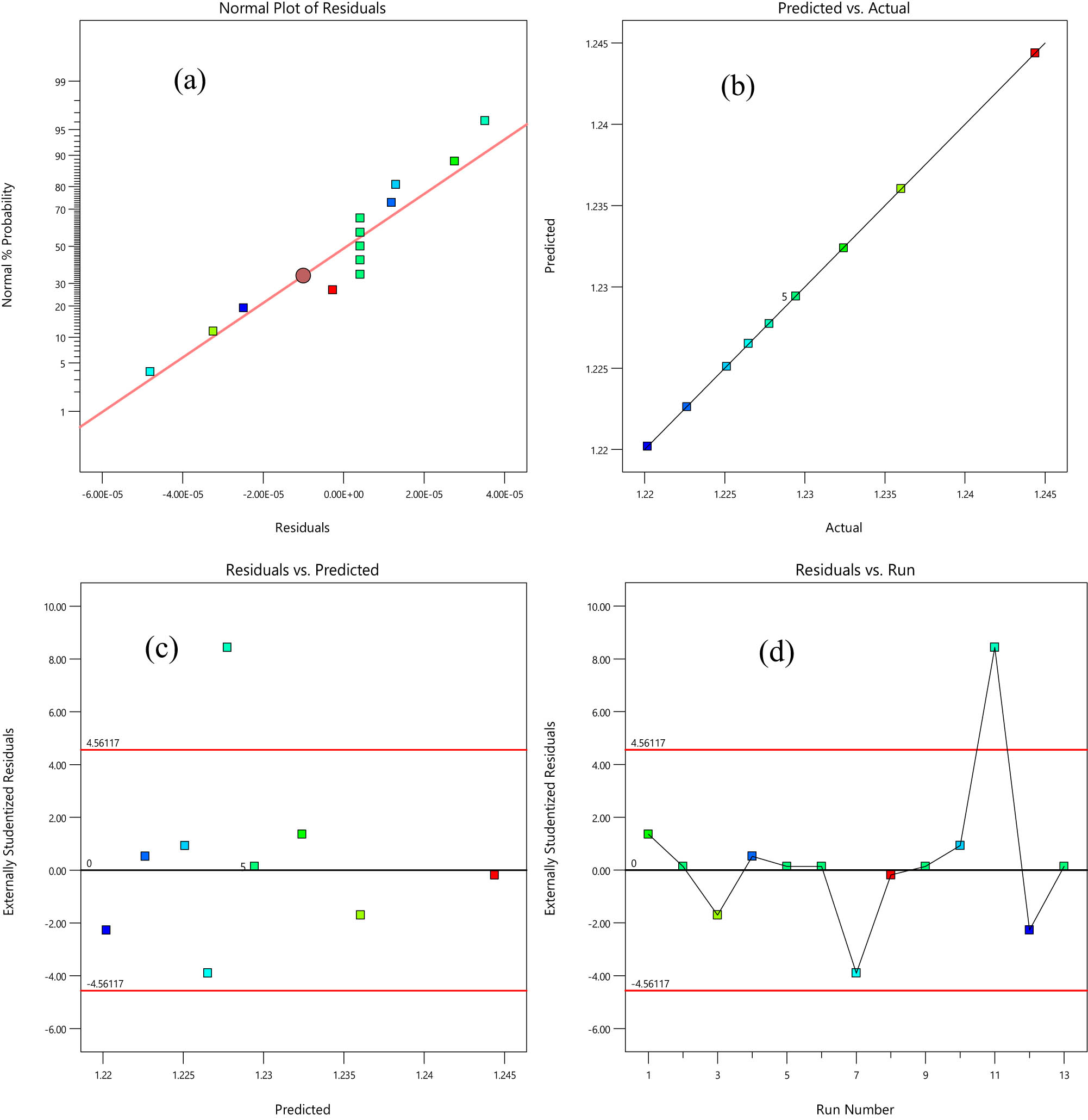
Residual plots for sheet thickness: (a) normal probability, (b) goodness of fit, (c) studentized residuals against predicted, and (d) studentized residuals against run number.

Residual plots for share stress: (a) normal probability, (b) goodness of fit, (c) studentized residuals against predicted, and (d) studentized residuals against run number.
The forecast values vs particular actual ones for
Based on a mathematical framework developed through RSM, response surface plots given in Figure 5(a)–(f) provide a two- and three-dimensional visualization of the relationship in the middle of independent variables along with a specific response variable in the systems. These plots illustrate how variations in the independent variables, represented on the

Contour and 3D surface response plot of
In the calendering process, optimization focuses on achieving key targets: maximizing a particular heat transfer rate (represented by the

Optimum solution with desirability.
Residual plots are essential diagnostic tools in regression analysis. They allow for the examination of model assumptions. By analyzing residuals, one can assess the goodness-of-fit of a model and identify potential areas for improvement or data issues, such as outliers or patterns that the model fails to capture. So, the residual plots for the

Residual plots for Nusselt number.

Residual plots for sheet thickness.

Residual plots for shear stress.
Finally, the ANOVA and model summary for
ANOVA for
| Source | DF | Adj SS | Adj MS | F-value | P-value |
|---|---|---|---|---|---|
| Model | 4 | 0.002688 | 0.000672 | 28496.93 | 0.000 |
| Linear | 2 | 0.002441 | 0.001221 | 51765.22 | 0.000 |
| We | 1 | 0.001863 | 0.001863 | 79023.59 | 0.000 |
| M | 1 | 0.000578 | 0.000578 | 24506.84 | 0.000 |
| Square | 1 | 0.000000 | 0.000000 | 1.04 | 0.338 |
| We*We | 1 | 0.000000 | 0.000000 | 1.04 | 0.338 |
| 2-way interaction | 1 | 0.000247 | 0.000247 | 10456.25 | 0.000 |
| We*m | 1 | 0.000247 | 0.000247 | 10456.25 | 0.000 |
| Error | 8 | 0.000000 | 0.000000 | ||
| Lack of fit | 4 | 0.000000 | 0.000000 | * | * |
| Pure error | 4 | 0.000000 | 0.000000 | ||
| Total | 12 |
Model dummary appropriate to
| S | R-sq | R-sq(adj) | R-sq(pred) |
|---|---|---|---|
| 0.0001536 | 99.99% | 99.99% | 99.97% |
ANOVA for sheet thickness
| Source | DF | Adj SS | Adj MS | F-value | P-value |
|---|---|---|---|---|---|
| Model | 5 | 0.000437 | 0.000087 | 96017.21 | 0.000 |
| Linear | 2 | 0.000321 | 0.000161 | 176338.09 | 0.000 |
| We | 1 | 0.000052 | 0.000052 | 56727.36 | 0.000 |
| M | 1 | 0.000270 | 0.000270 | 295948.82 | 0.000 |
| Square | 2 | 0.000000 | 0.000000 | 16.68 | 0.002 |
| We*We | 1 | 0.000000 | 0.000000 | 1.80 | 0.222 |
| m*m | 1 | 0.000000 | 0.000000 | 32.56 | 0.001 |
| 2-way interaction | 1 | 0.000116 | 0.000116 | 127376.52 | 0.000 |
| We*m | 1 | 0.000116 | 0.000116 | 127376.52 | 0.000 |
| Error | 7 | 0.000000 | 0.000000 | ||
| Lack of fit | 3 | 0.000000 | 0.000000 | * | * |
| Pure error | 4 | 0.000000 | 0.000000 | ||
| Total | 12 | 0.000437 |
Model abstract for sheet thickness
| S | R-sq | R-sq(adj) | R-sq(pred) |
|---|---|---|---|
| 0.0000302 | 100.00% | 100.00% | 99.99% |
ANOVA for shear stress
| Source | DF | Adj SS | Adj MS | F-value | P-value |
|---|---|---|---|---|---|
| Model | 5 | 0.039849 | 0.007970 | 3872.01 | 0.000 |
| Linear | 2 | 0.037064 | 0.018532 | 9003.54 | 0.000 |
| We | 1 | 0.031561 | 0.031561 | 15333.46 | 0.000 |
| M | 1 | 0.005503 | 0.005503 | 2673.62 | 0.000 |
| Square | 2 | 0.000005 | 0.000002 | 1.18 | 0.362 |
| We*We | 1 | 0.000001 | 0.000001 | 0.41 | 0.540 |
| m*m | 1 | 0.000002 | 0.000002 | 1.09 | 0.331 |
| 2-way interaction | 1 | 0.002780 | 0.002780 | 1350.60 | 0.000 |
| We*m | 1 | 0.002780 | 0.002780 | 1350.60 | 0.000 |
| Error | 7 | 0.000014 | 0.000002 | ||
| Lack of fit | 3 | 0.000014 | 0.000005 | * | * |
| Pure error | 4 | 0.000000 | 0.000000 | ||
| Total | 12 | 0.039863 |
Model abstract for shear stress
| S | R-sq | R-sq(adj) | R-sq(pred) |
|---|---|---|---|
| 0.0014347 | 99.96% | 99.94% | 99.64% |
7.3 Sensitivity analysis
Nusselt number, sheet thickness, and shear stress are important in hydrodynamics and calendering processes. Regression Eqs. (52) and (55) are the basis for calculating the sensitivity. The term “sensitivity functions” refers to the restricted derivatives of a certain response variable with regard to the factor variables. They exist as follows:
where
Sensitivity analysis data for
|
|
B:m |
|
|
|
|
|
|
|---|---|---|---|---|---|---|---|
| −1 | 0.5 | −0.013697 | 0.010827 | 0.0002467 | 0.010827 | −0.059346 | 0.010827 |
| 2.5 | 0.002005 | 0.011741 | −0.010527 | 0.011741 | −0.006622 | 0.011741 | |
| 4.5 | 0.017707 | 0.012655 | −0.0213 | 0.012655 | 0.046103 | 0.012655 | |
| 0 | 0.5 | −0.013697 | 0.013967 | 0.0002662 | 0.013967 | −0.059346 | 0.013967 |
| 2.5 | 0.002005 | 0.014881 | −0.010507 | 0.014881 | −0.006622 | 0.014881 | |
| 4.5 | 0.017707 | 0.015795 | −0.02128 | 0.015795 | 0.046103 | 0.015795 | |
| 1 | 0.5 | −0.013697 | 0.017107 | 0.0002857 | 0.017107 | −0.059346 | 0.017107 |
| 2.5 | 0.002005 | 0.018021 | −0.010488 | 0.018021 | −0.006622 | 0.018021 | |
| 4.5 | 0.017707 | 0.018935 | −0.021261 | 0.018935 | 0.046103 | 0.018935 |

Sensitivity analysis of
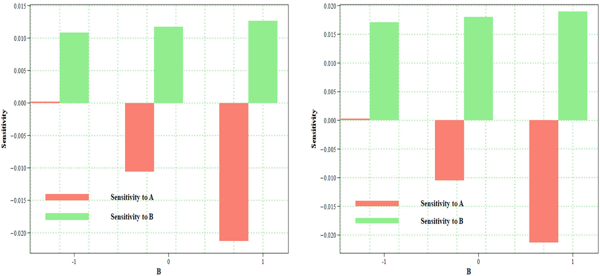
Sensitivity analysis of
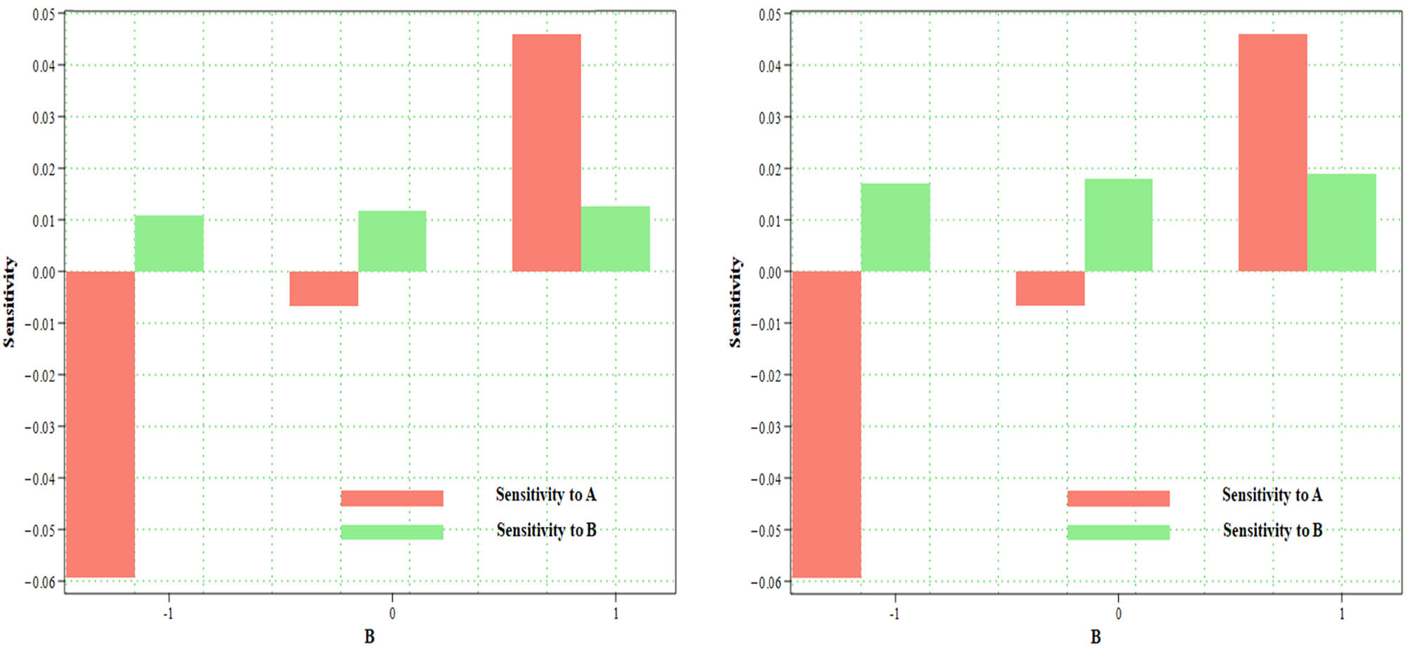
Sensitivity analysis of
8 Results and discussions
This section explains how the involved parameters for an incompressible EP fluid model whose viscosity is temperature-dependent during the calendering process affect the flow velocity, pressure gradient, power input pressure, and streamline graphically. The tables show a certain numeric result for the roll-separating force, leave of point, and the final sheet thickness for the various values of involved parameters.
Physical parameters are involved in the coating process [36].
| Parameters | Values | Unit |
|---|---|---|
|
|
1.2 × 10⁻⁴ – 7.6 × 10⁻⁶ |
|
|
|
0.2–5 |
|
|
|
0.1…0.15 |
|
|
|
850…1,200 |
|
|
|
0.1. 0.9 | |
|
|
0.5…4.5 | |
|
|
0.1…0.9 |
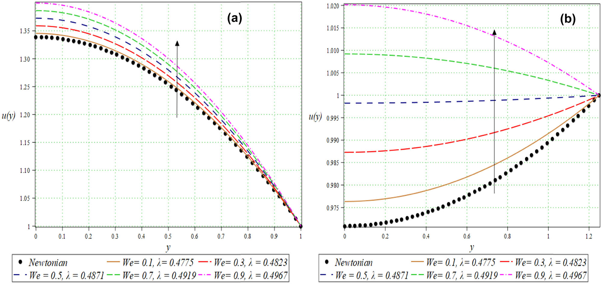
The impact of several parameters on velocity profile


Temperature distribution opposed to

Temperature distribution opposed to
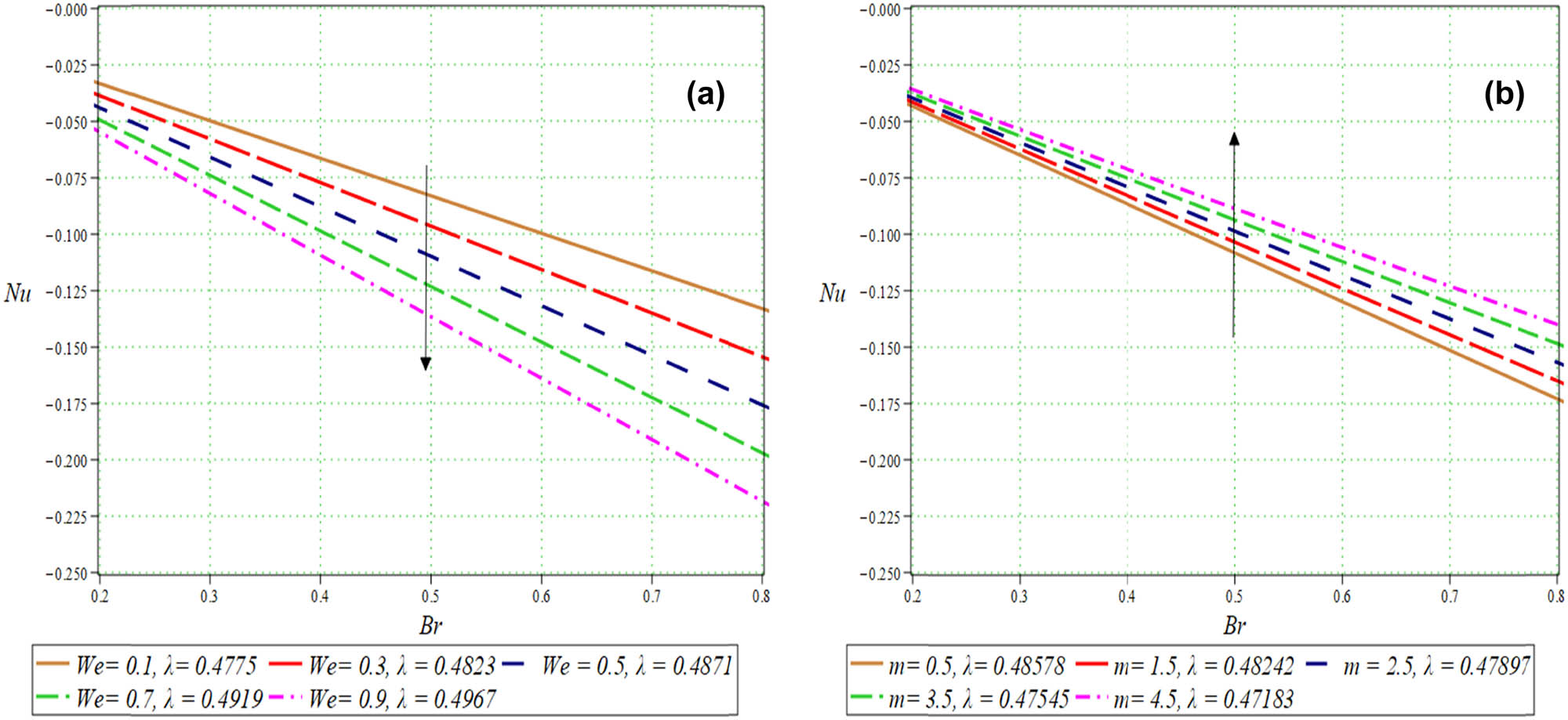
Figure 14(a) illustrates the significant impact of the temperature-dependent viscosity parameter
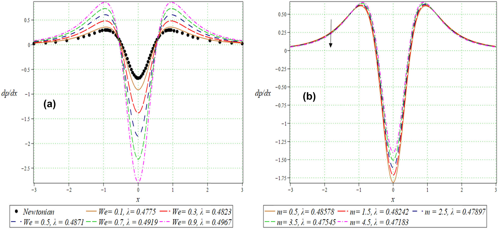
The pressure gradient
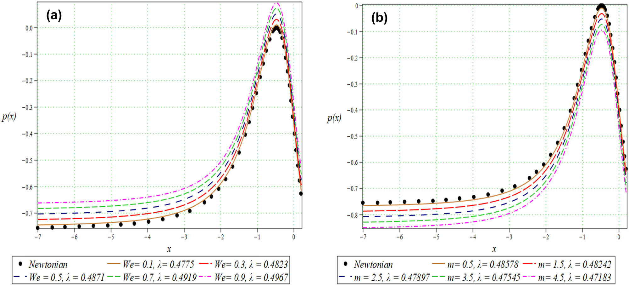
The pressure profile, which is the variation of pressure across the roll gap, is influenced by the
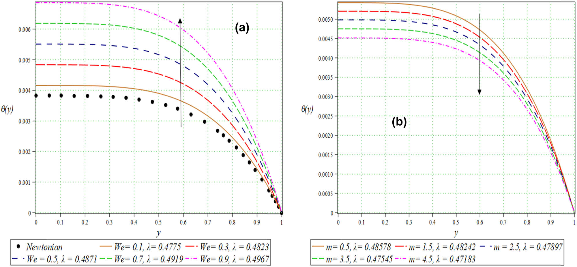
The temperature profile
In Figure 20(a), we observe the consequence of increasing a specific
Effect of
|
|
|
|
|
|---|---|---|---|
| 0.1 | 0.47752 | 1.2280 | −6.754281 |
| 0.2 | 0.47992 | 1.2303 | −6.756111 |
| 0.3 | 0.48232 | 1.2326 | −6.757941 |
| 0.4 | 0.48472 | 1.2349 | −6.759770 |
| 0.5 | 0.48712 | 1.2372 | −6.761599 |
| 0.6 | 0.48952 | 1.2396 | −6.763428 |
| 0.7 | 0.49192 | 1.2419 | −6.765262 |
| 0.8 | 0.49432 | 1.2443 | −6.767085 |
| 0.9 | 0.49672 | 1.2467 | −6.768913 |
Effect of
|
|
|
|
|
|---|---|---|---|
| 0.5 | 0.48578 | 1.2359 | −6.76099 |
| 1 | 0.48411 | 1.2343 | −6.75727 |
| 1.5 | 0.48242 | 1.2327 | −6.75761 |
| 2 | 0.48071 | 1.2310 | −6.75787 |
| 2.5 | 0.47897 | 1.2294 | −6.75392 |
| 3 | 0.47722 | 1.2277 | −6.75403 |
| 3.5 | 0.47545 | 1.2260 | −6.75404 |
| 4 | 0.47365 | 1.2243 | −6.74988 |
| 4.5 | 0.47183 | 1.2226 | −6.74973 |
9 Conclusions
This study presents a comprehensive theoretical investigation into the influence of various factors on the temperature-dependent viscosity of an Eyring–Powell fluid flowing between two equally sized rolls rotating at identical speeds in a calendering process. By applying an appropriate transformation, the dimensional momentum and energy-governing equations were converted into a non-dimensional form and simplified using the lubrication approximation theory. The resulting nonlinear ordinary differential equations were analytically solved using a perturbation method. The accuracy of the RSM approach was found to be approximately 99%, which was employed to generate 3D surface plots and 2D contour plots. The fluid flow characteristics, analyzed in terms of key parameters, were presented through tables and graphs, offering valuable insights.
The study revealed that the maximum fluid velocity occurs at the mid-region of the calender gap. An increase in the viscosity parameter was observed to reduce the detachment point, sheet thickness, pressure gradient, and pressure profile. Conversely, an increase in the Brinkman number enhanced the velocity profile while decreasing the temperature distribution. Additionally, the viscosity parameter significantly influenced the Nusselt number, thereby impacting heat transfer efficiency.
These findings enhance the understanding of heat transfer and flow dynamics in the calendering process of Eyring–Powell fluids, providing practical insights for optimizing industrial applications. The study also lays a solid foundation for future research in this area.
Acknowledgments
This work was supported by the Deanship of Scientific Research, Vice Presidency for Graduate Studies and Scientific Research, King Faisal University, Saudi Arabia (Grant No. 252105). Also, this research was supported by the Talent Project of Tianchi Young-Doctoral Program in Xinjiang Uygur Autonomous Region of China (Grant No. 51052401510).
-
Funding information: This work was supported by the Deanship of Scientific Research, Vice Presidency for Graduate Studies and Scientific Research, King Faisal University, Saudi Arabia (Grant No. 252105).
-
Author contributions: The idea was created and integrated into a mathematical model by F.A. & M.Z.; F.A. solved the problem; F.A. and M.F. wrote the manuscript; B.S., N.A.T., F.A. and A.A.F. highlighted the physics involved in the problem and added to the discussion of it; S.S.K.R., F.A., and M.W.A. reviewed, edited, and helped with the English corrections. All authors have accepted responsibility for the entire content of this manuscript and approved its submission.
-
Conflict of interest: The authors state no conflict of interest.
-
Data availability statement: Data sharing is not applicable to this article as no datasets were generated or analyzed during the current study.
References
[1] Javed M, Akram R, Nazeer M, Ghaffari A. Heat transfer analysis of the non-Newtonian polymer in the calendering process with slip effects. Int J Mod Phys B. 2024;38:2450105.10.1142/S0217979224501054Search in Google Scholar
[2] Ardichvili G. An attempt at a rational determination of the ambering of calender rolls. Kautschuk. 1938;14:23–5.Search in Google Scholar
[3] Paslay P. Calendering of a viscoelastic material. J Appl Mech. 1957;24(4):602–8.10.1115/1.4011607Search in Google Scholar
[4] Bergen J, Scott Jr G. Pressure distribution in the calendering of plastic materials. J Appl Mech. 1951;18(1):101–6.10.1115/1.4010227Search in Google Scholar
[5] Gaskell R. The calendering of plastic materials. J Appl Mech. 1950;17(3):334–6.10.1115/1.4010136Search in Google Scholar
[6] Kiparissides C, Vlachopoulos J. Finite element analysis of calendering. Polym Eng Sci. 1976;16:712–9.10.1002/pen.760161010Search in Google Scholar
[7] Tadmor Z, Gogos CG. Principles of polymer processing. Hoboken, New Jersey, USA: John Wiley & Sons; 2013.Search in Google Scholar
[8] Brazinsky I, Cosway H, Valle Jr C, Jones RC, Story V. A theoretical study of liquid‐film spread heights in the calendering of Newtonian and power law fluids. J Appl Polym Sci. 1970;14:2771–84.10.1002/app.1970.070141111Search in Google Scholar
[9] Alston Jr WW, Astill KN. An analysis for the calendering of non‐Newtonian fluids. J Appl Polym Sci. 1973;17:3157–74.10.1002/app.1973.070171018Search in Google Scholar
[10] Middleman S. Fundamentals of polymer processing. New York: McGraw-Hill; 1977.Search in Google Scholar
[11] Soong DS. Polymer processing. Chem Eng Educ. 1981;15:204–7.Search in Google Scholar
[12] Zheng R, Tanner R. A numerical analysis of calendering. J Non-Newtonian Fluid Mech. 1988;28:149–70.10.1016/0377-0257(88)85037-7Search in Google Scholar
[13] Mitsoulis E, Vlachopoulos J, Mirza F. Calendering analysis without the lubrication approximation. Polym Eng Sci. 1985;25:6–18.10.1002/pen.760250103Search in Google Scholar
[14] Arcos J, Méndez F, Bautista O. Effect of temperature-dependent consistency index on the exiting sheet thickness in the calendering of power-law fluids. Int J Heat Mass Transf. 2011;54:3979–86.10.1016/j.ijheatmasstransfer.2011.04.027Search in Google Scholar
[15] Sofou S, Mitsoulis E. Calendering of pseudoplastic and viscoplastic sheets of finite thickness. J Plastic Film Sheeting. 2004;20:185–222.10.1177/8756087904047660Search in Google Scholar
[16] Hatzikiriakos SG. Professor E. Mitsoulis’s contributions to rheology and computational non-Newtonian fluid mechanics. J Non-Newtonian Fluid Mech. 2023;311:104973.10.1016/j.jnnfm.2022.104973Search in Google Scholar
[17] Arcos J, Bautista O, Méndez F, Bautista E. Sensitivity of calendered thickness to temperature variations for Newtonian fluids. Eur J Mech-B/Fluids. 2012;36:97–103.10.1016/j.euromechflu.2012.03.012Search in Google Scholar
[18] Zahid M, Rana M, Siddiqui A, Haroon T. Modeling of non-isothermal flow of a magnetohydrodynamic, viscoplastic fluid during calendering. J Plastic Film Sheeting. 2016;32:74–96.10.1177/8756087915579304Search in Google Scholar
[19] Hernández A, Arcos J, Méndez F, Bautista O. Effect of pressure-dependent viscosity on the exiting sheet thickness in the calendering of Newtonian fluids. Appl Math Model. 2013;37:6952–63.10.1016/j.apm.2013.02.010Search in Google Scholar
[20] Arcos J, Bautista O, Méndez F, Bautista E. Theoretical analysis of the calendered exiting thickness of viscoelastic sheets. J Non-Newtonian Fluid Mech. 2012;177:29–36.10.1016/j.jnnfm.2012.04.004Search in Google Scholar
[21] Ali N, Javed MA, Sajid M. Theoretical analysis of the exiting thickness of sheets in the calendering of FENE-P fluid. J Non-Newtonian Fluid Mech. 2015;225:28–36.10.1016/j.jnnfm.2015.09.005Search in Google Scholar
[22] Calcagno B, Hart K, Crone W. Calendering of metal/polymer composites: an analytical formulation. Mech Mater. 2016;93:257–72.10.1016/j.mechmat.2015.10.017Search in Google Scholar
[23] Zahid M, Ali F, Souayeh B, Khan MT. Influence of variable viscosity on existing sheet thickness in the calendering of non-isothermal viscoelastic materials. Open Phys. 2024;22:20240023.10.1515/phys-2024-0023Search in Google Scholar
[24] Ali N, Javed MA, Atif HM. Non-isothermal analysis of calendering using couple stress fluid. J Plastic Film Sheeting. 2018;34:358–81.10.1177/8756087917746454Search in Google Scholar
[25] Ali F, Hou Y, Zahid M, Rana MA. Mathematical analysis of pseudoplastic polymers during reverse roll-coating. Polymers. 2020;12:2285.10.3390/polym12102285Search in Google Scholar PubMed PubMed Central
[26] Akinshilo AT, Olaye O. On the analysis of the Erying Powell model based fluid flow in a pipe with temperature dependent viscosity and internal heat generation. J King Saud Univ-Eng Sci. 2019;31:271–9.10.1016/j.jksues.2017.09.001Search in Google Scholar
[27] Ali F, Narasimhamurthy S, Hegde S, Usman M. Temperature-dependent viscosity analysis of Powell–Eyring fluid model during a roll-over web coating process. Polymers. 2024;16:1723.10.3390/polym16121723Search in Google Scholar
[28] Darbari B, Rashidi S, Abolfazli Esfahani J. Sensitivity analysis of entropy generation in nanofluid flow inside a channel by response surface methodology. Entropy. 2016;18:52.10.3390/e18020052Search in Google Scholar
[29] Javed MA, Ali N, Sajid M. A theoretical analysis of the calendering of Ellis fluid. J Plastic Film Sheeting. 2017;33:207–26.10.1177/8756087916647998Search in Google Scholar
[30] Javed MA, Ali N, Arshad S, Nawaz S, Ghaffari A. Theoretical investigation of a fluid model in calendering process involving slip at the upper roll surface. ZAMM‐J Appl Math Mech/Z Angew Math Mech. 2023;103:e202100406.10.1002/zamm.202100406Search in Google Scholar
[31] Abbas Z, Khaliq S. Calendering analysis of non-isothermal viscous nanofluid containing Cu-water nanoparticles using two counter-rotating rolls. J Plastic Film Sheeting. 2021;37:182–204.10.1177/8756087920951614Search in Google Scholar
[32] Javed MA, Asghar Z, Atif HM, Nisar M. A computational study of the calendering processes using Oldroyd 8-constant fluid with slip effects. Polym Polym Compos. 2023;31:09673911231202888.10.1177/09673911231202888Search in Google Scholar
[33] Patel M, Timol M. Numerical treatment of Powell–Eyring fluid flow using method of satisfaction of asymptotic boundary conditions (MSABC). Appl Numer Math. 2009;59:2584–92.10.1016/j.apnum.2009.04.010Search in Google Scholar
[34] Hussain F, Subia GS, Nazeer M, Ghafar M, Ali Z, Hussain A. Simultaneous effects of Brownian motion and thermophoretic force on Eyring–Powell fluid through porous geometry. Z Naturforsch A. 2021;76:569–80.10.1515/zna-2021-0004Search in Google Scholar
[35] Nazeer M, Ahmad F, Saeed M, Saleem A, Naveed S, Akram Z. Numerical solution for flow of a Eyring–Powell fluid in a pipe with prescribed surface temperature. J Braz Soc Mech Sci Eng. 2019;41:518.10.1007/s40430-019-2005-3Search in Google Scholar
[36] Abbas Z, Khaliq S. Numerical study of non-isothermal analysis of exiting sheet thickness in the calendering of micropolar-Casson fluid. J Plastic Film Sheeting. 2022;38:105–29.10.1177/87560879211025080Search in Google Scholar
© 2025 the author(s), published by De Gruyter
This work is licensed under the Creative Commons Attribution 4.0 International License.
Articles in the same Issue
- Research Articles
- Single-step fabrication of Ag2S/poly-2-mercaptoaniline nanoribbon photocathodes for green hydrogen generation from artificial and natural red-sea water
- Abundant new interaction solutions and nonlinear dynamics for the (3+1)-dimensional Hirota–Satsuma–Ito-like equation
- A novel gold and SiO2 material based planar 5-element high HPBW end-fire antenna array for 300 GHz applications
- Explicit exact solutions and bifurcation analysis for the mZK equation with truncated M-fractional derivatives utilizing two reliable methods
- Optical and laser damage resistance: Role of periodic cylindrical surfaces
- Numerical study of flow and heat transfer in the air-side metal foam partially filled channels of panel-type radiator under forced convection
- Water-based hybrid nanofluid flow containing CNT nanoparticles over an extending surface with velocity slips, thermal convective, and zero-mass flux conditions
- Dynamical wave structures for some diffusion--reaction equations with quadratic and quartic nonlinearities
- Solving an isotropic grey matter tumour model via a heat transfer equation
- Study on the penetration protection of a fiber-reinforced composite structure with CNTs/GFP clip STF/3DKevlar
- Influence of Hall current and acoustic pressure on nanostructured DPL thermoelastic plates under ramp heating in a double-temperature model
- Applications of the Belousov–Zhabotinsky reaction–diffusion system: Analytical and numerical approaches
- AC electroosmotic flow of Maxwell fluid in a pH-regulated parallel-plate silica nanochannel
- Interpreting optical effects with relativistic transformations adopting one-way synchronization to conserve simultaneity and space–time continuity
- Modeling and analysis of quantum communication channel in airborne platforms with boundary layer effects
- Theoretical and numerical investigation of a memristor system with a piecewise memductance under fractal–fractional derivatives
- Tuning the structure and electro-optical properties of α-Cr2O3 films by heat treatment/La doping for optoelectronic applications
- High-speed multi-spectral explosion temperature measurement using golden-section accelerated Pearson correlation algorithm
- Dynamic behavior and modulation instability of the generalized coupled fractional nonlinear Helmholtz equation with cubic–quintic term
- Study on the duration of laser-induced air plasma flash near thin film surface
- Exploring the dynamics of fractional-order nonlinear dispersive wave system through homotopy technique
- The mechanism of carbon monoxide fluorescence inside a femtosecond laser-induced plasma
- Numerical solution of a nonconstant coefficient advection diffusion equation in an irregular domain and analyses of numerical dispersion and dissipation
- Numerical examination of the chemically reactive MHD flow of hybrid nanofluids over a two-dimensional stretching surface with the Cattaneo–Christov model and slip conditions
- Impacts of sinusoidal heat flux and embraced heated rectangular cavity on natural convection within a square enclosure partially filled with porous medium and Casson-hybrid nanofluid
- Stability analysis of unsteady ternary nanofluid flow past a stretching/shrinking wedge
- Solitonic wave solutions of a Hamiltonian nonlinear atom chain model through the Hirota bilinear transformation method
- Bilinear form and soltion solutions for (3+1)-dimensional negative-order KdV-CBS equation
- Solitary chirp pulses and soliton control for variable coefficients cubic–quintic nonlinear Schrödinger equation in nonuniform management system
- Influence of decaying heat source and temperature-dependent thermal conductivity on photo-hydro-elasto semiconductor media
- Dissipative disorder optimization in the radiative thin film flow of partially ionized non-Newtonian hybrid nanofluid with second-order slip condition
- Bifurcation, chaotic behavior, and traveling wave solutions for the fractional (4+1)-dimensional Davey–Stewartson–Kadomtsev–Petviashvili model
- New investigation on soliton solutions of two nonlinear PDEs in mathematical physics with a dynamical property: Bifurcation analysis
- Mathematical analysis of nanoparticle type and volume fraction on heat transfer efficiency of nanofluids
- Creation of single-wing Lorenz-like attractors via a ten-ninths-degree term
- Optical soliton solutions, bifurcation analysis, chaotic behaviors of nonlinear Schrödinger equation and modulation instability in optical fiber
- Chaotic dynamics and some solutions for the (n + 1)-dimensional modified Zakharov–Kuznetsov equation in plasma physics
- Fractal formation and chaotic soliton phenomena in nonlinear conformable Heisenberg ferromagnetic spin chain equation
- Single-step fabrication of Mn(iv) oxide-Mn(ii) sulfide/poly-2-mercaptoaniline porous network nanocomposite for pseudo-supercapacitors and charge storage
- Novel constructed dynamical analytical solutions and conserved quantities of the new (2+1)-dimensional KdV model describing acoustic wave propagation
- Tavis–Cummings model in the presence of a deformed field and time-dependent coupling
- Spinning dynamics of stress-dependent viscosity of generalized Cross-nonlinear materials affected by gravitationally swirling disk
- Design and prediction of high optical density photovoltaic polymers using machine learning-DFT studies
- Robust control and preservation of quantum steering, nonlocality, and coherence in open atomic systems
- Coating thickness and process efficiency of reverse roll coating using a magnetized hybrid nanomaterial flow
- Dynamic analysis, circuit realization, and its synchronization of a new chaotic hyperjerk system
- Decoherence of steerability and coherence dynamics induced by nonlinear qubit–cavity interactions
- Finite element analysis of turbulent thermal enhancement in grooved channels with flat- and plus-shaped fins
- Modulational instability and associated ion-acoustic modulated envelope solitons in a quantum plasma having ion beams
- Statistical inference of constant-stress partially accelerated life tests under type II generalized hybrid censored data from Burr III distribution
- On solutions of the Dirac equation for 1D hydrogenic atoms or ions
- Entropy optimization for chemically reactive magnetized unsteady thin film hybrid nanofluid flow on inclined surface subject to nonlinear mixed convection and variable temperature
- Stability analysis, circuit simulation, and color image encryption of a novel four-dimensional hyperchaotic model with hidden and self-excited attractors
- A high-accuracy exponential time integration scheme for the Darcy–Forchheimer Williamson fluid flow with temperature-dependent conductivity
- Novel analysis of fractional regularized long-wave equation in plasma dynamics
- Development of a photoelectrode based on a bismuth(iii) oxyiodide/intercalated iodide-poly(1H-pyrrole) rough spherical nanocomposite for green hydrogen generation
- Investigation of solar radiation effects on the energy performance of the (Al2O3–CuO–Cu)/H2O ternary nanofluidic system through a convectively heated cylinder
- Quantum resources for a system of two atoms interacting with a deformed field in the presence of intensity-dependent coupling
- Studying bifurcations and chaotic dynamics in the generalized hyperelastic-rod wave equation through Hamiltonian mechanics
- A new numerical technique for the solution of time-fractional nonlinear Klein–Gordon equation involving Atangana–Baleanu derivative using cubic B-spline functions
- Interaction solutions of high-order breathers and lumps for a (3+1)-dimensional conformable fractional potential-YTSF-like model
- Hydraulic fracturing radioactive source tracing technology based on hydraulic fracturing tracing mechanics model
- Numerical solution and stability analysis of non-Newtonian hybrid nanofluid flow subject to exponential heat source/sink over a Riga sheet
- Numerical investigation of mixed convection and viscous dissipation in couple stress nanofluid flow: A merged Adomian decomposition method and Mohand transform
- Effectual quintic B-spline functions for solving the time fractional coupled Boussinesq–Burgers equation arising in shallow water waves
- Analysis of MHD hybrid nanofluid flow over cone and wedge with exponential and thermal heat source and activation energy
- Solitons and travelling waves structure for M-fractional Kairat-II equation using three explicit methods
- Impact of nanoparticle shapes on the heat transfer properties of Cu and CuO nanofluids flowing over a stretching surface with slip effects: A computational study
- Computational simulation of heat transfer and nanofluid flow for two-sided lid-driven square cavity under the influence of magnetic field
- Irreversibility analysis of a bioconvective two-phase nanofluid in a Maxwell (non-Newtonian) flow induced by a rotating disk with thermal radiation
- Hydrodynamic and sensitivity analysis of a polymeric calendering process for non-Newtonian fluids with temperature-dependent viscosity
- Exploring the peakon solitons molecules and solitary wave structure to the nonlinear damped Kortewege–de Vries equation through efficient technique
- Modeling and heat transfer analysis of magnetized hybrid micropolar blood-based nanofluid flow in Darcy–Forchheimer porous stenosis narrow arteries
- Activation energy and cross-diffusion effects on 3D rotating nanofluid flow in a Darcy–Forchheimer porous medium with radiation and convective heating
- Insights into chemical reactions occurring in generalized nanomaterials due to spinning surface with melting constraints
- Influence of a magnetic field on double-porosity photo-thermoelastic materials under Lord–Shulman theory
- Soliton-like solutions for a nonlinear doubly dispersive equation in an elastic Murnaghan's rod via Hirota's bilinear method
- Analytical and numerical investigation of exact wave patterns and chaotic dynamics in the extended improved Boussinesq equation
- Nonclassical correlation dynamics of Heisenberg XYZ states with (x, y)-spin--orbit interaction, x-magnetic field, and intrinsic decoherence effects
- Exact traveling wave and soliton solutions for chemotaxis model and (3+1)-dimensional Boiti–Leon–Manna–Pempinelli equation
- Unveiling the transformative role of samarium in ZnO: Exploring structural and optical modifications for advanced functional applications
- On the derivation of solitary wave solutions for the time-fractional Rosenau equation through two analytical techniques
- Analyzing the role of length and radius of MWCNTs in a nanofluid flow influenced by variable thermal conductivity and viscosity considering Marangoni convection
- Advanced mathematical analysis of heat and mass transfer in oscillatory micropolar bio-nanofluid flows via peristaltic waves and electroosmotic effects
- Exact bound state solutions of the radial Schrödinger equation for the Coulomb potential by conformable Nikiforov–Uvarov approach
- Some anisotropic and perfect fluid plane symmetric solutions of Einstein's field equations using killing symmetries
- Nonlinear dynamics of the dissipative ion-acoustic solitary waves in anisotropic rotating magnetoplasmas
- Curves in multiplicative equiaffine plane
- Exact solution of the three-dimensional (3D) Z2 lattice gauge theory
- Propagation properties of Airyprime pulses in relaxing nonlinear media
- Symbolic computation: Analytical solutions and dynamics of a shallow water wave equation in coastal engineering
- Wave propagation in nonlocal piezo-photo-hygrothermoelastic semiconductors subjected to heat and moisture flux
- Comparative reaction dynamics in rotating nanofluid systems: Quartic and cubic kinetics under MHD influence
- Laplace transform technique and probabilistic analysis-based hypothesis testing in medical and engineering applications
- Physical properties of ternary chloro-perovskites KTCl3 (T = Ge, Al) for optoelectronic applications
- Gravitational length stretching: Curvature-induced modulation of quantum probability densities
- The search for the cosmological cold dark matter axion – A new refined narrow mass window and detection scheme
- A comparative study of quantum resources in bipartite Lipkin–Meshkov–Glick model under DM interaction and Zeeman splitting
- PbO-doped K2O–BaO–Al2O3–B2O3–TeO2-glasses: Mechanical and shielding efficacy
- Nanospherical arsenic(iii) oxoiodide/iodide-intercalated poly(N-methylpyrrole) composite synthesis for broad-spectrum optical detection
- Sine power Burr X distribution with estimation and applications in physics and other fields
- Numerical modeling of enhanced reactive oxygen plasma in pulsed laser deposition of metal oxide thin films
- Dynamical analyses and dispersive soliton solutions to the nonlinear fractional model in stratified fluids
- Computation of exact analytical soliton solutions and their dynamics in advanced optical system
- An innovative approximation concerning the diffusion and electrical conductivity tensor at critical altitudes within the F-region of ionospheric plasma at low latitudes
- An analytical investigation to the (3+1)-dimensional Yu–Toda–Sassa–Fukuyama equation with dynamical analysis: Bifurcation
- Swirling-annular-flow-induced instability of a micro shell considering Knudsen number and viscosity effects
- Review Article
- Examination of the gamma radiation shielding properties of different clay and sand materials in the Adrar region
- Erratum
- Erratum to “On Soliton structures in optical fiber communications with Kundu–Mukherjee–Naskar model (Open Physics 2021;19:679–682)”
- Special Issue on Fundamental Physics from Atoms to Cosmos - Part II
- Possible explanation for the neutron lifetime puzzle
- Special Issue on Nanomaterial utilization and structural optimization - Part III
- Numerical investigation on fluid-thermal-electric performance of a thermoelectric-integrated helically coiled tube heat exchanger for coal mine air cooling
- Special Issue on Nonlinear Dynamics and Chaos in Physical Systems
- Analysis of the fractional relativistic isothermal gas sphere with application to neutron stars
- Abundant wave symmetries in the (3+1)-dimensional Chafee–Infante equation through the Hirota bilinear transformation technique
- Successive midpoint method for fractional differential equations with nonlocal kernels: Error analysis, stability, and applications
- Novel exact solitons to the fractional modified mixed-Korteweg--de Vries model with a stability analysis